The low-level radial velocity variability in
Barnard’s star (=GJ 699)

We report results from $2\leavevmode\nobreak\ 1/2\leavevmode\nobreak\ {\rm yr}$ of high precision radial velocity (RV) monitoring of Barnard’s star. The high RV measurement precision of the VLT-UT2+UVES of $2.65\leavevmode\nobreak\ {\rm m\leavevmode\nobreak\ s}^{-1}$ made the following findings possible. (1) The first detection of the change in the RV of a star caused by its space motion (RV secular acceleration). (2) An anti-correlation of the measured RV with the strength of the filling-in of the ${\rm H}_{\alpha}$ line by emission. (3) Very stringent mass upper limits to planetary companions. Using only data from the first 2 years, we obtain a best-fit value for the RV secular acceleration of $5.15\pm 0.89\leavevmode\nobreak\ {\rm m\leavevmode\nobreak\ s}^{-1}\leavevmode\nobreak\ {\rm yr}^{-1}$. This agrees within $0.95\sigma$ with the predicted value of $4.50\leavevmode\nobreak\ {\rm m\leavevmode\nobreak\ s}^{-1}\leavevmode\nobreak\ {\rm yr}^{-1}$ based on the Hipparcos proper motion and parallax combined with the known absolute radial velocity of the star. When the RV data of the last half-year are added the best-fit slope is strongly reduced to $2.97\pm 0.51\leavevmode\nobreak\ {\rm m\leavevmode\nobreak\ s}^{-1}\leavevmode\nobreak\ {\rm yr}^{-1}$ ($3.0\sigma$ away from the predicted value), clearly suggesting the presence of additional RV variability in the star. Part of it can be attributed to stellar activity as we demonstrate by correlating the residual RVs with an index that describes the filling-in of the H_α line by emission. A correlation coefficient of $-0.50$ indicates that the appearance of active regions causes a blueshift of photospheric absorption lines. Assuming that active regions basically inhibit convection we discuss the possibility that the fundamental (inactive) convection pattern in this M4V star produces a convective redshift which would indicate that the majority of the absorption lines relevant for our RV measurements is formed in a region of convective overshoot. This interpretation could possibly extend a trend indicated in the behaviour of earlier spectral types that exhibit convective blueshift, but with decreasing line asymmetries and blueshifts as one goes from G to K dwarfs. Based on this assumption, we estimate that the variation of the visible plage coverage is about $20\%$. We also determine upper limits to the projected mass $m\sin i$ and to the true mass $m$ of hypothetical planetary companions in circular orbits. For the separation range $0.017-0.98\leavevmode\nobreak\ {\rm AU}$ we exclude any planet with $m\sin i>0.12\leavevmode\nobreak\ {\rm M}_{\rm Jupiter}$ and $m>0.86\leavevmode\nobreak\ {\rm M}_{\rm Jupiter}$. Throughout the habitable zone around Barnard’s star, i.e. $0.034-0.082\leavevmode\nobreak\ {\rm AU}$, we exclude planets with $m\sin i>7.5\leavevmode\nobreak\ {\rm M}_{\rm Earth}$ and $m>3.1\leavevmode\nobreak\ {\rm M}_{\rm Neptune}$.

1 Introduction

The search for extrasolar planets via precise stellar radial velocity (RV) measurements has led to more than 100 discovery announcements up to now (e.g. Mayor & Queloz 1995; Marcy & Butler 1996; Kürster et al. 2000). A good fraction of these discoveries is summarized in the paper by Butler et al. (2002). The majority of the extrasolar planets has so far been found around main sequence stars of spectral types from late–F through K. There is only one M dwarf with planetary companions known, GJ876, which is orbited by two Jovian-type planets with orbital periods of $30.1$ and $61.0\leavevmode\nobreak\ {\rm day}$, respectively (Marcy et al. 2001; Delfosse et al. 1998). Combining RV data with new astrometric measurements Benedict et al. (2002) determine a mass of $1.89\pm 0.34\leavevmode\nobreak\ {\rm M}_{\rm Jupiter}$ for the outer planet.

It is due to the intrinsic faintness of M dwarfs that this most abundant type of star tends to be underrepresented in RV searches as very high measurement precision requires large telescopes. This introduces a strong bias in any attempt to estimate the frequency of planetary companions to stars as a whole.

On the other hand, due to the low mass of M dwarfs an orbiting planet of a given mass causes a higher reflex motion of the star. Therefore, the present day measurement precision for differential radial velocities (DRV) of a few ${\rm m\leavevmode\nobreak\ s}^{-1}$ holds the prospect to discover terrestrial planets (with a few Earth masses) in close-in orbits around the lower mass M dwarfs, e.g. in their habitable zones (Schneider 1998; Endl et al. 2003).

For instance, for a main sequence star with a mass of $0.16\leavevmode\nobreak\ {\rm M}_{\odot}$, such as that of Barnard’s star, the subject of the present paper (mass from Henry et al. 1999), the habitable zone lies at $0.034-0.082\leavevmode\nobreak\ {\rm AU}$ (see Kasting et al. 1991) corresponding to orbital periods in the range $5.75-21.5\leavevmode\nobreak\ {\rm d}$. Around a star of this mass a planet in a circular orbit with a projected mass $m\sin i=1\leavevmode\nobreak\ {\rm M}_{\rm Earth}$ would cause a peak-to-peak RV amplitude of $2.4\leavevmode\nobreak\ {\rm m\leavevmode\nobreak\ s}^{-1}$ at the inner edge of the habitable zone and $1.6\leavevmode\nobreak\ {\rm m\leavevmode\nobreak\ s}^{-1}$ at its outer edge. For $m\sin i=3\leavevmode\nobreak\ {\rm M}_{\rm Earth}$ the resulting peak-to-peak RV amplitudes would be $7.3\leavevmode\nobreak\ {\rm m\leavevmode\nobreak\ s}^{-1}$ and $4.7\leavevmode\nobreak\ {\rm m\leavevmode\nobreak\ s}^{-1}$, respectively.

When attempting to measure such small RV signals it becomes important to consider other effects that affect the determination of DRVs. Two such effects are important for M dwarfs. First, the high proper motion of nearby stars causes a secular change in their RV which for some stars can reach several ${\rm m\leavevmode\nobreak\ s}^{-1}$ within a few years. Second, intrinsic variability due to stellar activity can mimic RV variations. Little is known so far about the level at which this complicates DRV measurements in M dwarfs.

This paper reports on high precision DRV measurements obtained with VLT-UT2+UVES of Barnard’s star which, as we demonstrate, exhibits a considerable secular change of its RV. It is known as a quite inactive star and was selected with the expectation that its DRV measurements are largely unaffected by activity; as we shall see this is not the case.

The paper is structured as follows. We summarize the known properties of Barnard’s star (Sect. 2) and proceed with a description of the concept of RV secular acceleration (Sect. 3). Our observations are described in Sect. 4 along with a brief outline of our data modelling technique. In Sect. 5 we present results on the RV secular acceleration, on the relation between DRVs and stellar activity as evidenced in the strength of the H_α line, and on period analysis in the RV and ${\rm H}_{\alpha}$ data; we also provide mass upper limits to planetary companions. We discuss our results in Sect. 6 and summarize our conclusions in Sect. 7.

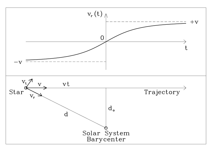
Figure 1: Lower panel: Geometry of the space motion of a passing star. $v_{\rm t}$ and $v_{\rm r}$ are, respectively, the transversal and radial components of the space velocity $v$. The current distance is $d$, the minimum distance is $d_{\circ}$, and $vt$ is the trajectory from the current position to the point of nearest approach. Upper panel: The ARV as a function of time and its asymptotic limits $\pm v$.

2 Properties of Barnard’s star

The M4V dwarf Barnard’s star (GJ 699, HIP 87937) is the nearest star after Proxima Centauri and the $\alpha$ Centauri binary. Its parallax has been determined by Hipparcos as $549.01\pm 1.58\leavevmode\nobreak\ {\rm mas}$ (ESA 1997; Perryman et al. 1997), i.e. the distance is $1.8215\pm 0.0052\leavevmode\nobreak\ {\rm pc}$. Barnard’s star has long been known as the highest proper motion star in the sky (Barnard 1916, 1917). For epoch 1991.25 Hipparcos gives $\mu_{\alpha}=-797.84\leavevmode\nobreak\ {\rm mas\leavevmode\nobreak\ yr}^{-1}$ and $\mu_{\delta}=10326.93\leavevmode\nobreak\ {\rm mas\leavevmode\nobreak\ yr}^{-1}$ for the proper motion in right ascension and declination, respectively (ESA 1997). The tangential component of the space velocity (perpendicular to the line of sight) is thus $v_{\rm t}=89.440\leavevmode\nobreak\ {\rm km\leavevmode\nobreak\ s}^{-1}$. The secular change of the proper motion is $1.2\leavevmode\nobreak\ {\rm mas\leavevmode\nobreak\ yr}^{-2}$ (Gatewood 1995).

Barnard’s star also has a high ARV. Dravins et al. (1999) find an astrometrically derived ARV of $v_{\rm r}=-101.9\pm 6.5\leavevmode\nobreak\ {\rm km\leavevmode\nobreak\ s}^{-1}$, somewhat smaller (in absolute value) than the spectroscopic value of $-110.506\leavevmode\nobreak\ {\rm km\leavevmode\nobreak\ s}^{-1}$ by Nidever et al. (2001) who estimate their systematic errors in their treatment of gravitational redshift and convective blueshift) to $0.4\leavevmode\nobreak\ {\rm km\leavevmode\nobreak\ s}^{-1}$. Other spectroscopic literature values are, e.g., $-110.9\pm 0.2\leavevmode\nobreak\ {\rm km\leavevmode\nobreak\ s}^{-1}$ (García-Sanchez et al. 2001) and $-109.7\leavevmode\nobreak\ {\rm km\leavevmode\nobreak\ s}^{-1}$ (Turon et al. 1998). Thus the overall space velocity is $v\approx 142\leavevmode\nobreak\ {\rm km\leavevmode\nobreak\ s}^{-1}$. In the following we will adopt the ARV value by Nidever et al. (2001) noting that none of the results presented in this paper would be significantly altered, if, e.g., we took the astrometric ARV value by Dravins et al. (1999). The same would be true, if we replaced the Hipparcos astrometric data by the recently refined values by Benedict et al. (1999) who used the Fine Guidance Sensor 3 of the Hubble Space Telescope for interferometric fringe tracking astrometry.

Due to its high space motion and sub-solar metallicity Gizis (1997) classifies Barnard’s star as an “Intermediate Pop. II star” (following Majewski 1993), i.e. an object between a halo star and a thin disk star. Its low observed X-ray luminosity (Marino et al. 2000; Hünsch et al. 1999) and its presumable rotation period of $130.4\leavevmode\nobreak\ {\rm d}$ (from weak evidence for $\approx 0\aas@@fstack{m}01$ photometric variations by Benedict et al. 1998) also indicate an inactive old star.

Table 1: Kinematic data for Barnard’s star. For all data used in our calculation (Hip = Hipparcos, Nid = Nidever et al. 2001, UV = our UVES data) we list the epoch, the distance $d$, the ARV $v_{\rm r}$, and the secular acceleration of the RV ${\rm d}v_{\rm r}/{\rm d}t$. We also compare our results for the point of closest approach (CA) with those of García-Sanchez et al. 2001 (GS).

Data/	Epoch	$\leavevmode\nobreak\ \leavevmode\nobreak\ \leavevmode\nobreak\ \leavevmode\nobreak\ d$	$v_{\rm r}$	${\rm d}v_{\rm r}/{\rm d}t$
Event		$\leavevmode\nobreak\ \leavevmode\nobreak\ [{\rm pc}]$	$[{\rm kms}^{-1}]$	$[{\rm ms}^{-1}{\rm yr}^{-1}]$
Hip	$\leavevmode\nobreak\ 1991.25$	$1.8215$	$-110.532$	$\leavevmode\nobreak\ 4.491$
Nid	$\leavevmode\nobreak\ 1996.91$	$1.8209$	$-110.506$	$\leavevmode\nobreak\ 4.496$
UV	$\leavevmode\nobreak\ 2001.51$	$1.8203$	$-110.485$	$\leavevmode\nobreak\ 4.499$
CA	$11730$	$1.1458$	$\leavevmode\nobreak\ \leavevmode\nobreak\ \leavevmode\nobreak\ 0.0$	$18.043$
GS	$11700_{{}^{\pm 100}}$	$1.144_{{}^{\pm 0.005}}$	$\leavevmode\nobreak\ \leavevmode\nobreak\ \leavevmode\nobreak\ (0.0)$	not given

For many years Barnard’s star was also a prime candidate for displaying astrometric pertubations attributable to one or two planetary companions in long-period orbits of about $12$ and $20\leavevmode\nobreak\ {\rm yr}$ (van de Kamp 1963, 1982). This was later refuted by Gatewood (1995). The most recent astrometric measurements by Benedict et al. (1999) placed stringent mass upper limits of $2.1\leavevmode\nobreak\ {\rm M}_{\rm Jupiter}$ down to $0.37\leavevmode\nobreak\ {\rm M}_{\rm Jupiter}$ for orbital periods of $50\leavevmode\nobreak\ {\rm d}$ up to $600\leavevmode\nobreak\ {\rm d}$ (see Fig. 8 in Sect. 5.4).

3 The secular acceleration of the radial velocity

The proximity and high space velocity of Barnard’s star implies a detectable secular change of its radial velocity (RV secular acceleration; van de Kamp 1977). To illustrate this effect Fig. 1 (lower panel) shows the trajectory past the barycenter of the solar system of a star in linear space motion, i.e. ignoring the subtle variations of the galactic potential (see García-Sanchez et al. 2001). The minimum distance $d_{\circ}$ at the point of closest approach is given by

$$d_{\circ}=\frac{d}{\sqrt{1+v_{\rm r}^{2}/v_{\rm t}^{2}}}\leavevmode\nobreak\ ,$$ (1)

where $d$, $v_{\rm t}$, and $v_{\rm r}$ are the distance, and the tangential and radial velocity components, respectively, at some earlier epoch. The time $t$ at the earlier epoch is

$$t=t_{\circ}-\frac{\sqrt{d^{2}-d_{\circ}^{2}}}{v}\leavevmode\nobreak\ ,$$ (2)

where $v=\sqrt{v_{\rm r}^{2}+v_{\rm t}^{2}}$ is the space velocity and $t_{\circ}$ is the time at closest approach. Setting $t_{\circ}=0$ the ARV as a function of time is given by

$$v_{\rm r}(t)=\frac{v^{2}t}{\sqrt{v^{2}t^{2}+d_{\circ}^{2}}}\leavevmode\nobreak\ .$$ (3)

The upper panel of Fig. 1 shows a graph of this function. Differentiation yields the secular acceleration of the RV:

$$\frac{{\rm d}v_{\rm r}(t)}{{\rm d}t}=\frac{v^{2}}{\sqrt{v^{2}t^{2}+d_{\circ}^{2}}}-\frac{v^{4}t^{2}}{(v^{2}t^{2}+d_{\circ}^{2})^{3/2}}\leavevmode\nobreak\ .$$ (4)

Kinematic data for Barnard’s star using Eqs. (1–4) with the input data from Sect. 3 are summarized in Table 1 that lists the distance, the ARV, and its secular acceleration for the individual epochs of all measurements relevant to this paper. For the time of closest approach to the solar system our results are compared with those of García-Sanchez (2001).

At the mean time of our UVES observations presented here (epoch 2001.51) the RV secular acceleration is $4.499\leavevmode\nobreak\ {\rm m\leavevmode\nobreak\ s^{-1}\leavevmode\nobreak\ yr^{-1}}$. Over the time baseline for our UVES data of $2.422\leavevmode\nobreak\ {\rm yr}$ the acceleration value increases by only $0.0020\leavevmode\nobreak\ {\rm m\leavevmode\nobreak\ s^{-1}\leavevmode\nobreak\ yr^{-1}}$; we neglect this small increase and treat the secular acceleration as a purely linear function when comparing it to our UVES data.

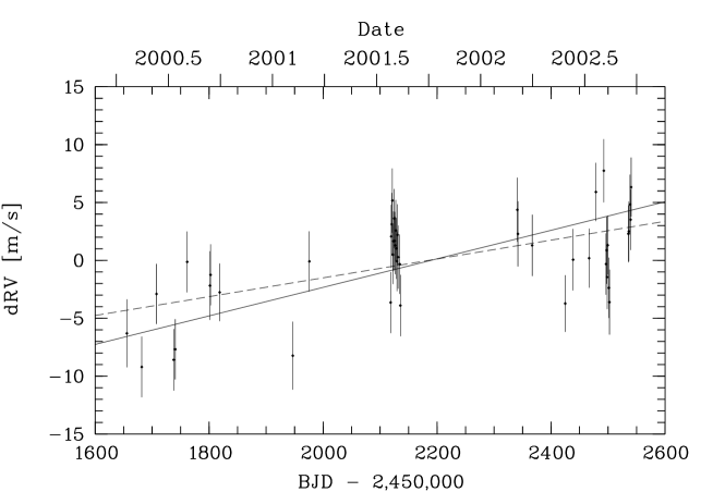
Figure 2:  Time series of the differential RV data of Barnard’s star plotted vs. Barycentric Julian Day (bottom) and the Date (top). The solid line represents the predicted RV secular acceleration of $4.499\leavevmode\nobreak\ {\rm m\leavevmode\nobreak\ s^{-1}\leavevmode\nobreak\ yr^{-1}}$. The dashed line is a linear fit to the data with a slope of $2.97\pm 0.51\leavevmode\nobreak\ {\rm m\leavevmode\nobreak\ s}^{-1}\leavevmode\nobreak\ {\rm yr}^{-1}$.

4 Observations and data modelling

Barnard’s star was observed with the VLT-UT2+UVES in the framework of our ongoing precision RV survey of M dwarfs in search for extrasolar planets. UVES was used together with its self-calibrating iodine gas absorption cell operated at a temperature of $70^{\circ}{\rm C}$. Image slicer #3 and an $0.3^{\prime\prime}$ slit were chosen yielding a resolving power of $R=100\,000-120\,000$. At the selected central wavelength of $600\leavevmode\nobreak\ {\rm nm}$ the useful spectral range containing iodine $(\mathrm{I}_{2})$ absorption lines ($\approx 500-600\leavevmode\nobreak\ {\rm nm}$) falls entirely on the better quality CCD of the mosaic of two $4\leavevmode\nobreak\ {\rm K}\times 2\leavevmode\nobreak\ {\rm K}$ CCDs.

Our analysis of the stellar spectra to determine differential radial velocities (DRV) followed Endl et al. (2000). Briefly, DRV measurements were made with the iodine cell inserted in the light path which produces a superposition of a forest of dense iodine absorption lines onto the stellar spectrum. A higher-resolution $(R=700\,000-1\,000\,000)$ template spectrum of the iodine cell obtained with the McMath Fourier Transform Spectrometer (FTS) on Kitt Peak was used to reconstruct the instrumental profile (IP) from observations of rapidly rotating B-stars through the iodine cell. This was required in one night for Maximum Entropy deconvolution (with the IP) of a pure stellar spectrum (taken without the iodine cell) in order to obtain a stellar template spectrum with a resolution matching that of the FTS iodine spectrum. Finally, both template spectra were combined to model the regular observations (star+iodine), again employing IP reconstruction. From the Doppler shift of these model spectra with respect to the stellar template we obtain a time series of the DRV of the star which is largely corrected for instrumental instabilities.

As the IP varies strongly within an Echelle order of UVES spectra as well as across the orders, the modelling was done in small spectral chunks of $\approx 0.2\leavevmode\nobreak\ {\rm nm}$ each of which yields an independent DRV measurement. DRV values from $\approx 580$ spectral segments (after rejection of outliers) were then averaged to produce the final DRV value for the spectrum; the error of this mean value was taken as the measurement error.

A total of 137 star+iodine spectra are available from 46 nights between 21 April 2000 and 23 Sept. 2002. Triplets of exposures were obtained each night within about 16 min, except for one night where only two spectra could be secured. Individual exposure times were $250-285\leavevmode\nobreak\ {\rm s}$ yielding a typical S/N per pixel of $66$. On average our error of the individual RV measurement is $2.65\leavevmode\nobreak\ {\rm m\leavevmode\nobreak\ s}^{-1}$ demonstrating the high precision achievable with UVES on this faint star $(V=9.54\leavevmode\nobreak\ {\rm mag})$. All RV data were corrected to the solar system barycenter using the JPL ephemeris DE200 (Standish 1990) for the flux-weighted temporal midpoint of the exposure as given by the UVES exposuremeter. For each epoch of observation proper motion corrected stellar coordinates were used.

A note on error estimation is in order at this point. As a multi-user instrument UVES in service mode undergoes frequent setup changes (central wavelength, slit width, image slicers, etc.). This can lead to systematic RV shifts of purely instrumental nature that may not be fully accounted for by our IP modelling approach. The IP will be more and more affected by setup changes when their number increases. Conversely, within a given night or on a time scale of a few nights higher instrumental stability can be expected. Errors estimated from the scatter in a single night are most likely not representative for the long-term error. On the other hand, errors estimated over time scales of a few nights may already be affected by real variability of the star.

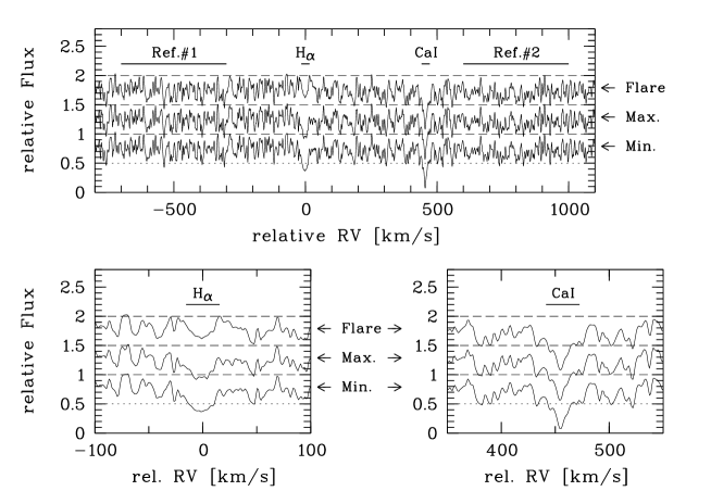
Figure 3:  A selection of nightly mean spectra of Barnard’s star near H${}_{\alpha}\leavevmode\nobreak\ 6563$ and CaI $6573$. Upper panel: three spectra are shown vertically offset. They correspond to the minimum H_α index (lower spectrum), the maximum “quiescent” H_α index (middle spectrum offset by 0.5 flux units), and the flare event (upper spectrum offset by 1.0 flux units). Lower panels: Zooms into the upper panel on H_α (left) and CaI (right). While a filling-in of the H_α line by emission can be seen, the CaI line is constant. Horizontal bars indicate the spectral regions over which average fluxes are determined for the line indices according to Eq. (5).

For this reason we chose to perform all subsequent analysis of our data on nightly mean values of the DRV (46 data points) in order to avoid an overestimation of the significances of possible signals. For the same reason we chose not to use the propagation of the errors of the individual nightly DRV values to obtain the error of the nightly mean DRV (which on average for all nights would be $1.54\leavevmode\nobreak\ {\rm m\leavevmode\nobreak\ s}^{-1}$); neither did we choose the RMS of the individual nightly DRV values around the mean for this purpose (which on average would give $1.39\leavevmode\nobreak\ {\rm m\leavevmode\nobreak\ s}^{-1}$). Instead we chose the mean of the individual errors to represent the error of the nightly mean DRV (on average $2.65\leavevmode\nobreak\ {\rm m\leavevmode\nobreak\ s}^{-1}$). This choice may appear a bit conservative and arbitrary, but we estimate that it leads to more realistic values for the nightly errors as it is to a large extent the imperfection of our IP reconstruction that is reflected in the error of the individual measurement and should therefore also be reflected in the nightly error.

Table 2: Models for the UVES data of Barnard’s star: constant, predicted secular acceleration (S.A.), and linear fit. For each model we list the slope, the RMS scatter of the data around the model, the $\chi^{2}$ of the fit, the degrees of freedom (dof), and the associated probability. The RMS values should be compared with the mean internal measurement error of $2.65\leavevmode\nobreak\ {\rm ms}^{-1}$. The last line corresponds to a model based on the predicted secular acceleration together with a linear correlation with the ${\rm H}_{\alpha}$ line strength index defined in Sect. 5.2.

Model	Slope	RMS	$\chi^{2}$	dof	$p$
	$[{\rm ms}^{-1}{\rm yr}^{-1}]$	$[{\rm ms}^{-1}]$
Const.a	$(0.0)$	3.93	97.2	45	$1.3\cdot 10^{-5}$
S.A.a	$4.499$	3.38	72.3	45	$0.0065$
Lin. fita	$2.97\pm 0.51$	3.17	63.4	44	$0.029$
Lin. fitb	$5.15\pm 0.89$	2.70	29.0	28	$0.41$
S.A.+${{\rm H}_{\alpha}}^{\rm c}$	$(4.499)$	2.94	54.4	43	$0.12$

• Data from all 46 nights.

• Data from the first 2 years only (first 30 nights).

• Data from all nights excluding flare event (45 nights).

5 Results

5.1 RV secular acceleration

Fig. 2 shows the time series of our DRV data of Barnard’s star. Each data point represents the nightly average of the DRV. The predicted secular acceleration of the RV (Sect. 3) is overplotted as a solid line (zero point matched). The dotted line represents a linear fit to the data.

The best-fit linear trend yields a slope of $2.97\pm 0.51\leavevmode\nobreak\ {\rm m\leavevmode\nobreak\ s}^{-1}\leavevmode\nobreak\ {\rm yr}^{-1}$ somewhat smaller (by $3.0\sigma$) than the predicted secular acceleration of $4.499\leavevmode\nobreak\ {\rm m\leavevmode\nobreak\ s}^{-1}\leavevmode\nobreak\ {\rm yr}^{-1}$. Clearly, a constant model is rejected as it would be $5.8\sigma$ away from the fitted slope. For each model the slope and RMS scatter of the data around it are listed in Table 2 together with the $\chi^{2}$, degrees of freedom, and associated probability.

The relatively small formal probability of the secular acceleration model $(0.65\%)$ indicates that additional variability is present in our data. The linear fit attempts to account for part of this variability. If only the data of the first 2 years are used for a linear fit ($BJD<2\leavevmode\nobreak\ 452\leavevmode\nobreak\ 000$, i.e. the first 30 nights) the resulting slope is $5.15\pm 0.98\leavevmode\nobreak\ {\rm m\leavevmode\nobreak\ s}^{-1}\leavevmode\nobreak\ {\rm yr}^{-1}$ which agrees within $0.95\sigma$ with the predicted secular acceleration (not shown in Fig. 2). Around $BJD=2\leavevmode\nobreak\ 452\leavevmode\nobreak\ 500$ we had intensified the observations in an attempt to obtain a better sampling of a suspected minimum in the RV residuals from the secular acceleration model. The presence of this minimum had been suggested by period analysis and the minimum was clearly found, but it added more weight to negative residual DRV values thereby reducing the slope of the linear fit.

5.2 Correlation between H_α line strength and RVs

In order to find out whether stellar activity is the source of, or a contributor to, the observed RV variability we examined the filling-in by chromospheric emission of the H_α absorption line in an attempt to find a correlation with the DRV data. H_α ($6562.808$ Å) is the only activity indicator in the wavelength regime encompassed by our UVES spectra. Filling-in of the core of this absorption line is an indicator for chromospheric plage, i.e. active regions where magnetic fields are important for the convective properties of the star and where star spots may also influence the shape of photospheric absorption lines.

M dwarf spectra are very rich in absorption lines which blend and do not show a continuum between them which makes it difficult to obtain precise absolute line fluxes. Since, however, only relative fluxes are of interest here we define a suitable line index by

$$I=\frac{\overline{F_{\circ}}}{0.5*(\overline{F_{1}}+\overline{F_{2}})}\leavevmode\nobreak\ ,$$ (5)

where $\overline{F_{\circ}}$ is the mean spectral flux in a selected RV interval around the line to be studied. For the ${\rm H}_{\alpha}$ line we chose the RV interval $[-15.5,+15.5\leavevmode\nobreak\ {\rm km\leavevmode\nobreak\ s}^{-1}]$ centered on the core of the line. $\overline{F_{1}}$ and $\overline{F_{2}}$ are the mean fluxes in two reference bandpasses on either side of H_α (assumed to exhibit only negligible variability with the appearance of active regions) for which we chose the intervals $[-700,-300\leavevmode\nobreak\ {\rm km\leavevmode\nobreak\ s}^{-1}]$ and $[+600,+1000\leavevmode\nobreak\ {\rm km\leavevmode\nobreak\ s}^{-1}]$, respectively. These velocities are corrected for the barycentric Earth motion (cf. Sect. 3) and for the ARV of Barnard’s star (Sect. 2).

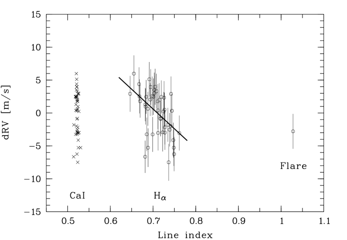
Figure 4: DRV (after subtraction of the secular acceleration) vs. spectral line index (see text). Circles with RV error bars: DRV vs. ${\rm H}_{\alpha}$ index. Crosses: DRV vs. CaI index. The line represents a linear fit to the DRV vs. ${\rm H}_{\alpha}$ index relation. The rightmost data point correpsonds to the flare event.

For comparison we evaluated the line index for a nearby CaI line at $6572.795$ Å with low excitation potential that is very strong in M dwarfs and whose line strength is not expected to have a significant dependance on stellar activity. For this line we chose $F_{\circ}$ over the RV range $[+441.5,+472.5\leavevmode\nobreak\ {\rm km\leavevmode\nobreak\ s}^{-1}]$ (again relative to ${\rm H}_{\alpha}$). Should our data reduction have produced systematic flux offsets, e.g. due to imperfect subtraction of the Echelle background, we should see them in the CaI line.

Fig. 3 shows three of our (nightly mean) spectra of Barnard’s star near the ${\rm H}_{\alpha}\leavevmode\nobreak\ 6563$ and CaI $6573$ lines. They correspond to the spectrum with the smallest ${\rm H}_{\alpha}$ index (labelled “Min.”), to the spectrum with the largest “quiescent” ${\rm H}_{\alpha}$ index (labelled “Max.”) and to the spectrum of a flare event with an ${\rm H}_{\alpha}$ index that is almost $12\sigma$ larger than the mean index of the remainder of the data (see also Fig. 4). Horizontal bars in Fig. 3 indicate the spectral regions over which the mean fluxes for Eq. (5) were determined.

The variation of the ${\rm H}_{\alpha}$ line strength can be seen as filling-in by emission, whereas the CaI line is constant. Interestingly, the smallest ${\rm H}_{\alpha}$ index was observed in the night following the flare event. It appears that either the flare occured on a quite inactive (visible) hemisphere or that the flare event has disrupted a major active region (just as solar flares cause a reconfiguration of the local magnetic fields). Since we have no data from the night before the flare these possibilities must remain speculation.

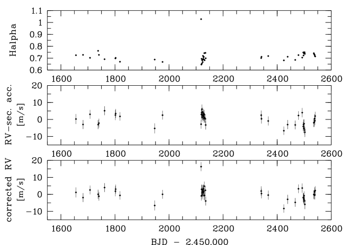
Figure 5: Comparison of DRV time series and time series of ${\rm H}_{\alpha}$ indices. Top: Time series of ${\rm H}_{\alpha}$ indices. Center: DRV time series (secular acceleration subtracted); RMS$=3.39\leavevmode\nobreak\ {\rm m\leavevmode\nobreak\ s}^{-1}$ (excluding flare event). Bottom: Time series of DRV values corrected for the linear correlation with the ${\rm H}_{\alpha}$ index displayed in Fig. 4; RMS$=2.94\leavevmode\nobreak\ {\rm m\leavevmode\nobreak\ s}^{-1}$ (excluding flare).

Fig. 4 shows a correlation of our DRV measurements (secular acceleration subtracted) with the ${\rm H}_{\alpha}$ and CaI indices. Just as the DRV values also the line indices were determined in the individual spectra of each night and then binned into nightly averages. Again, the CaI line is seen constant and independent from the DRV, but the ${\rm H}_{\alpha}$ line strength is variable and anti-correlated with the DRV. The flare event is seen only in ${\rm H}_{\alpha}$, but not in the CaI index. The relative scatter of the line indices is $0.54\%$ for CaI and $7.6\%$ for ${\rm H}_{\alpha}$ (or $3.8\%$ when the flare is excluded). The correlation coefficient is $-0.498$ (flare event excluded). A linear fit to the relation of DRV vs. ${\rm H}_{\alpha}$ index, $I({\rm H}_{\alpha})$, is given by ${\rm DRV}=(43\pm 10)\leavevmode\nobreak\ {\rm m\leavevmode\nobreak\ s}^{-1}-(60\pm 15)\leavevmode\nobreak\ {\rm m\leavevmode\nobreak\ s}^{-1}\leavevmode\nobreak\ I({\rm H}_{\alpha})$ . It reduces the total RMS of the DRV data (flare excluded) from $3.39\leavevmode\nobreak\ {\rm m\leavevmode\nobreak\ s}^{-1}$ to $2.94\leavevmode\nobreak\ {\rm m\leavevmode\nobreak\ s}^{-1}$. The probability of $\chi^{2}$ for this linear fit is $p=0.12$ rendering this model an acceptable description of the DRV data (see Table 2 for all numerical values of the fit).

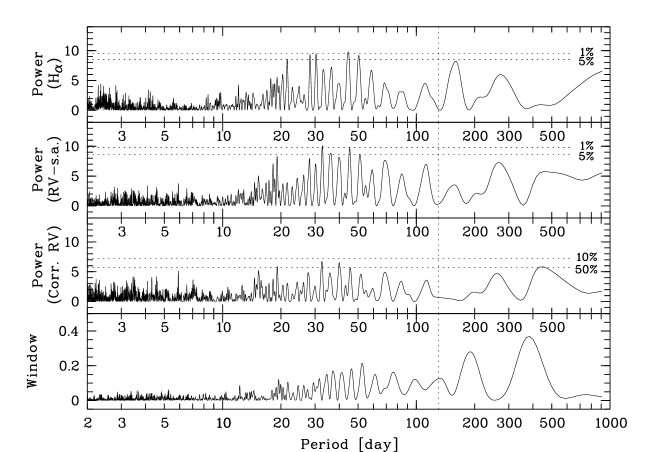
Figure 6:  Lomb-Scargle periodograms for our data of Barnard’s star. Top panel: ${\rm H}_{\alpha}$ index. Second panel from top: RV data (secular acceleration subtracted). Third panel: RV data additionally corrected for the correlation with the ${\rm H}_{\alpha}$ index. Bottom panel: window function. In each case the flare event was excluded from the data. Horizontal dotted lines indicate levels of the FAP ($1\%$ and $5\%$ in the upper two panels and $10\%$ and $50\%$ in the third). The vertical dotted line markes the supposed $130.4\leavevmode\nobreak\ {\rm d}$ rotation period by Benedict et al. (1998).

A technical note: near ${\rm H}_{\alpha}$ our spectra still contain weak iodine absorption lines from the iodine cell (cf. Sect. 4). The deepest iodine line in the wavelength regime relevant for our line indices has a depth of $9.3\%$ relative to the continuum; about half of this value is more typical for the average line. Due to the barycentric motion of the Earth, for which the chosen RV intervals are corrected (with correction extrema of $-26.4\leavevmode\nobreak\ {\rm km\leavevmode\nobreak\ s}^{-1}$ and $+26.2\leavevmode\nobreak\ {\rm km\leavevmode\nobreak\ s}^{-1}$) variable parts of the iodine spectrum contribute to the flux values in Eq. (5). Calculating the ${\rm H}_{\alpha}$ and CaI indices for a pure iodine spectrum (a flatfield exposure taken through the iodine cell) we obtain an RMS variation of $0.20\%$ and $0.17\%$ for the ${\rm H}_{\alpha}$ and CaI index, respectively, over the range of applied barycentric correction velocities. This intrinsic uncertainty is much smaller than the observed scatter of the line indices for our spectra of Barnard’s star ($3.8\%$ and $0.54\%$, respectively). Therefore, our neglection of the contribution of the weak iodine lines to these spectra does not introduce a major error in the determination of the line indices.

In Fig. 5 we show a comparison of the time series of our DRV data (secular acceleration subtracted) with the time series of the ${\rm H}_{\alpha}$ index. Also included in Fig. 5 is the time series of the DRV data corrected for the variation with ${\rm H}_{\alpha}$, i.e. after subtracting the linear fit shown in Fig. 4.

Even if the total scatter of the DRV data is reduced when the correlation with the ${\rm H}_{\alpha}$ index is applied for a correction, the basic variability pattern appears largely unchanged. Formally, the probability of $\chi^{2}$ provides an acceptable model, but we cannot exclude the possibility that our error estimates were too conservative (cf. Sect. 4). We should also note that we do not expect a simple linear correlation to be sufficient for a complete correction of the RV data for the effects of stellar activity.

Table 3: Period analysis results for the different data sets: ${\rm H}_{\alpha}$ index, RV after subtraction of the secular acceleration, RV additionally corrected for the linear correlation with the ${\rm H}_{\alpha}$ index, and window function. For the data sets that exclude the flare event the period values $P$ of the four highest periodogram peaks as well as the pertaining FAP are listed. Only for the RV data did we also evaluate period and FAP values with the flare event included. Similarity of a period value with an integer fraction of the photometric period by Benedict et al. (1998) is indicated in the last column.

Data set	$P\leavevmode\nobreak\ [{\rm d}]$	FAP	$P\leavevmode\nobreak\ [{\rm d}]$	FAP	Comment
	flare excluded		including flare
${\rm H}_{\alpha}$ index	44.5	0.82%			$\approx P_{\rm ph}/3$
	30.4	1.30%
	28.2	1.54%
	50.4	2.06%
RV	32.7	0.56%	32.7	1.56%	$\approx P_{\rm ph}/4$
	45.3	1.05%	45.3	4.27%	$\approx P_{\rm ph}/3$
			19.1	5.06%
	36.1	4.01%	36.0	8.26%
	51.1	5.49%
RV$-{\rm H}_{\alpha}$	32.5	36.81%			$\approx P_{\rm ph}/4$
	40.0	45.21%
	19.1	75.63%
	440	77.96%
Window	380	—			$\approx 1\leavevmode\nobreak\ {\rm yr}$
	190	—			$\approx 1/2\leavevmode\nobreak\ {\rm yr}$
	52.5	—
	46.2	—

5.3 Period analysis

We searched for periodic signals in the ${\rm H}_{\alpha}$ index, in the RV residuals from the secular acceleration model, and in the RV data after additional correction for the linear correlation with the ${\rm H}_{\alpha}$ index. We used the periodogram by Lomb (1976) and Scargle (1982) as well as a routine that employs $\chi^{2}$ fitting of sine waves. Contrary to the Lomb-Scargle method the sine fitting routine can adapt the RV zero point offset and also take into account data errors (cf. Cumming et al. 1999). The results of both methods do not differ substantially so that we only present the results from the Lomb-Scargle periodogram. Fig. 6 shows periodograms of the ${\rm H}_{\alpha}$ index, the RV residuals, and the RV data corrected for the correlation with ${\rm H}_{\alpha}$; the window function is also shown.

We searched the period range from $2\leavevmode\nobreak\ {\rm d}$ (our minimum temporal resolution) to $2.42\leavevmode\nobreak\ {\rm yr}$ (our total time baseline). False alarm probabilities (FAP) for the periodogram peaks were determined with a bootstrap randomization scheme (e.g. Kürster et al. 1997). $1\%$ and $5\%$ levels of the FAP are indicated in Fig. 6 for the periodograms of the ${\rm H}_{\alpha}$ and RV residuals. After correction with the ${\rm H}_{\alpha}$ correlation the power of the RV data was found considerably reduced; we display $10\%$ and $50\%$ FAP levels for this data set.

Table 3 lists the periods and FAPs of the four highest periodogram peaks for each of the three different data sets excluding the flare event as well as for the RV data including the flare event (pertaining periodogram not shown in Fig. 6). In none of the periodograms is there much power near the supposed photometric rotation period, $130.4\leavevmode\nobreak\ {\rm d}$, by Benedict et al. (1998) which is also indicated in Fig. 6 as a vertical dotted line. Nevertheless, the highest peaks tend to coincide with $1/3$ or $1/4$ of the photometric period value which may hint at a common origin.

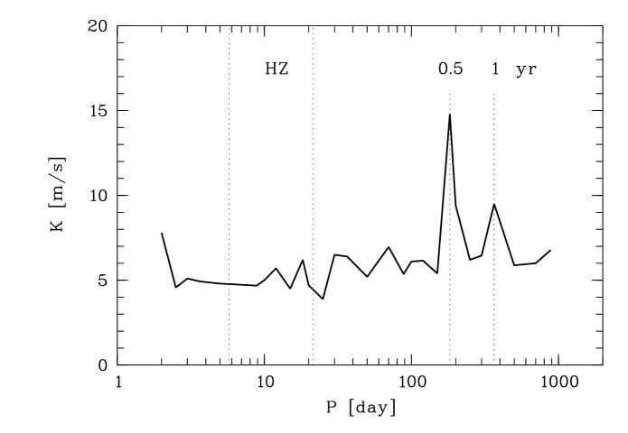
Figure 7: Upper limits to the RV semi-amplitude $K$ (for circular orbits) as a function of orbital period $P$. For each period value these limits correspond to the semi-amplitude at which the artificial signal was found at the $FAP\leq 1\%$ level for all 12 test phases. Two vertical dotted lines at periods of $5.75$ and $21.5\leavevmode\nobreak\ {\rm d}$ indicate the range of the habitable zone around Barnard’s star according to Kastings et al. (1991). Periods of $0.5$ and $1\leavevmode\nobreak\ {\rm yr}$ are also marked by vertical dotted lines; due to the structure of the data sampling relatively high limiting amplitudes result at these periods.

5.4 Upper limits to companion masses

Faced with the result that the observed RV variability appears to be attributable to stellar activity to a large extent and yields no evidence for orbiting companions we studied which types of companions can be excluded, i.e. we determined upper limits to the projected mass $m\sin i$ of orbiting companions (with $i$ the orbital inclination). To this end we determined the amplitudes of RV signals that we would have detected with $99\%$ confidence.

Again bootstrap randomization was employed. In the analysis artificial RV signals (see next paragraph for details) are added to the observed RV data which act as a noise term. Since on the one hand secular acceleration is a well understood effect, but on the other hand the linear correlation with the ${\rm H}_{\alpha}$ is probably not a complete description of the effect that activity exerts on RV measurements, we decided to use as the noise term the secular acceleration subtracted RV data including the flare event and uncorrected for the ${\rm H}_{\alpha}$ correlation. This data set has a higher rms scatter than the corrected one (see Table 2), i.e. it adds more noise to the test signals and yields more conservative upper limits. Note also that the highest peak in the periodogram of this data set itself (no signal added) appeared at $FAP=1.56\%$ (fifth column in Table 3) and would therefore not have passed the criterion of $99\%$ confidence that we adopt here.

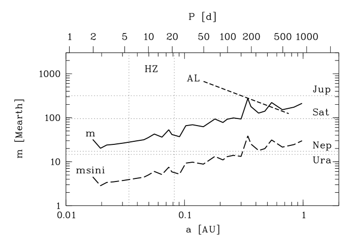
Figure 8: Upper limits to the mass $m$ of planetary companions in circular orbits around Barnard’s star plotted vs. star-planet separation $a$ (bottom) and orbital period $P$ (top). Long-dashed line labelled “msini”: $99\%$ confidence limits to the projected companion mass. Solid line labelled “m”: limits to the true companion mass based additionally on the $99\%$ confidence range for the inclination $i$; i.e. their combined confidence is $98\%$. Short-dashed line labelled “AL”: astrometric limits to $m$ from Benedict et al. (1999). Horizontal thin dotted lines indicate the masses of Jupiter, Saturn, Neptune, and Uranus. As in Fig. 7 the habitable zone according to Kasting et al. (1991) lies between the vertical thin dotted lines.

Sinusoids were used for the artificial signals rendering our analysis strictly valid only for circular orbits. We used 29 different period values encompassing the accessible period range $2\leavevmode\nobreak\ {\rm d}-2.42\leavevmode\nobreak\ {\rm yr}$. At each period 12 equally spaced phases were probed, and the amplitude of the sine wave was varied. The amplitude at which for a given input period the signal showed up at all 12 phases at the $FAP\leq 1\%$ level was taken as the minimum detectable amplitude. We did not require that the signal appear at the same period in the power spectrum (due to spectral leakage it not always did), but that it cause power with a chance probability $\leq 1\%$ somewhere in the search range.

Fig. 7 shows the resulting limiting RV semi-amplitudes as a function of orbital period. The median (mean) detectable RV semi-amplitude in the whole period search range is $5.88\leavevmode\nobreak\ (6.20)\leavevmode\nobreak\ {\rm m\leavevmode\nobreak\ s}^{-1}$; in the habitable zone it is $4.73\leavevmode\nobreak\ (5.07)\leavevmode\nobreak\ {\rm m\leavevmode\nobreak\ s}^{-1}$. These limits are smaller than any of the amplitudes found so far for extrasolar planets.

The amplitude limits were then converted to upper limits on the projected mass $m\sin i$ of planetary companions in circular orbits. A stellar mass of $0.16\leavevmode\nobreak\ {\rm M}_{\odot}$ was adopted from Henry et al. (1999). The limits on $m\sin i$ are shown as a function of period and star-planet separation in Fig. 8 (long-dashed line). To obtain limits to the full companion mass $m$ we used the probability (for random orientation of orbits) that the orbital inclination $i$ exceeds some angle $\theta$, given by $p(i>\theta)=\cos(\theta)$. In $99\%$ of the cases the true mass does not exceed the projected mass by more than a factor $7.088$. The solid line in Fig. 8 shows these mass limits which have a combined probability (that of signal detection and that of the inclination range) of $0.99^{2}\approx 98\%$. The short-dashed line labelled “AL” shows astrometric mass limits by Benedict et al.(1999) which are $99\%$ confidence limits, but allow for a $5\%$ miss rate for astrometric signals.

As seen in Fig. 8 the limits on $m\sin i$ increase roughly from a few Earth masses at the smallest separations to $\approx 30\leavevmode\nobreak\ {\rm M}_{\rm Earth}$ at larger separations. At periods of $1/2\leavevmode\nobreak\ {\rm yr}$ and $1\leavevmode\nobreak\ {\rm yr}$ we obtain somewhat higher limits because of lower detection capabilities due to the data sampling window.

6 Discussion

6.1 RV secular acceleration

We clearly find a positive trend in our DRV data of Barnard’s star and interpret it as mainly due to the secular acceleration of the RV. The formal discrepancy between a linear fit and the predicted secular acceleration value can be attributed to stellar acticity, in particular to incomplete sampling of the time scale(s) on which the activity varies.

To our knowledge this is the first reported observation of stellar RV secular acceleration. With time we expect the observed trend to conicide more with the predicted acceleration as activity effects cancel out more.

6.2 The activity-related RV signal: Evidence for convective redshift?

Active regions, which in our data reveal their appearance through the filling-in of the ${\rm H}_{\alpha}$ line core by emission, can affect the apparent stellar RV as measured in lines of photospheric origin by the effects of star spots or chromospheric plage regions. Compared to the inactive photosphere both spots and plage produce a local change of brightness and spectrum and also inhibit stellar convection locally by magnetic fields.

The primary effect of dark star spots at different locations on the visible stellar disk is a reduction of the observable flux at the instantaneous RV of the spot(s), as spot temperatures $T_{\rm s}$ are considerably smaller than photospheric effective temperatures $T_{\rm eff}$ and $(T_{\rm s}/T_{\rm eff})^{4}\ll 1$. Therefore, the effects that spots have a different spectrum and that convection is suppressed inside the spot have small contributions to the integrated stellar spectrum compared to the general flux reduction in a small RV regime. If there is sufficient rotational broadening of the absorption lines, then this will lead to a change in the center-of-gravity of the line thus mimicking an RV change. The effect is more pronounced when spots are displaced from the limb of the visible stellar disk where their instantaneous RV (relative to the RV of the star as a whole) is high. The effect disappears when spots are on the sub-observer meridian of the star where the relative RV is zero (or when they are on the invisible hemisphere of the star).

In a model that assumes that photospheric spots are surrounded by chromospheric plage the following picture emerges. Minimum RV shift, i.e. most active regions hidden from view or most active regions visible and concentrated towards the sub-observer meridian, should be accompanied by either small or large amounts of the filling-on of the ${\rm H}_{\alpha}$ line core by emission. Maximum RV shift, i.e. active regions concentrated on either side of the sub-observer meridian, should be seen when intermediate to large amounts of ${\rm H}_{\alpha}$ filling-in are observed (see also Paulson et al. 2002; Saar & Fischer 2000).

Consider the simple case of a single small spot on an otherwise featureless rotating star. Let $A_{\rm s}$ be the spot area and let $\phi$ be the rotation angle of the spot from the sub-observer meridian. The RV perturbation $\Delta v_{\rm r}$ then scales as $\Delta v_{\rm r}(\phi)\propto-A_{\rm s}f(\phi)g(\phi)v\sin i$, where $A_{\rm s}$ is the spot area, $f(\phi)$ is a function describing the visibility and foreshortening due to projection of the spot, hence $A_{\rm s}f(\phi)$ is the projected spot area, $g(\phi)$ is a function describing the deflection of the stellar RV caused by the spot as a function of stellar rotation phase $\phi$, and $v\sin i$ is the projected rotational velocity of the star. The minus sign indicates that the RV shift of the line as a whole is opposite to the instantaneous RV of the dark spot due to the flux reduction it produces.

Both $f(\phi)$ and $g(\phi)$ are periodic functions of $\phi$ which possess special symmetries around $\phi=0$, i.e. the phase where the spot is on the sub-observer meridian. The projection function $f(\phi)$ is mirror symmetric with respect to this phase (similar to a cosine function) while the RV deflection $g(\phi)$ has a rotational symmetry around this phase (just like a sine function does). In addition $g(\phi)$ has zero mean. Due to these properties of $f(\phi)$ and $g(\phi)$ the RV perturbation averaged over phase $\phi$ vanishes, i.e. $\langle\Delta v_{\rm r}\rangle=0$. On time scales longer than the stellar rotation period the mean spot related RV perturbation is therefore uncorrelated with the visibility of spots and spot coverage as indirectly evidenced by ${\rm H}_{\alpha}$ emission from the surrounding plage. It is only the scatter in the instantaneous RV deflection which correlates with spot visibility and area, but not the mean value.

In a plot of DRV vs. ${\rm H}_{\alpha}$ index one should thus expect for a single active region (small spot plus surrounding plage) a closed curve with a shape that resembles a “reclining raindrop”; if several active regions are present the plot contains a superposition of curves of this shape. If plage regions exist without underlying spots, the ${\rm H}_{\alpha}$ index will be further enhanced when they are visible without any spot-related effect on the RV, thus blurring the plot along its horizontal axis. In any case, if spots are responsible for the RV variability the correlation coefficient of the RV vs. ${\rm H}_{\alpha}$ relation should be close to zero. This is not evident in Fig. 4 so that star spots cannot be the dominant contributor to the observed correlation.

Estimates of the maximum spot contribution to $\Delta v_{\rm r}$ are consistent with this. Saar & Donahue (1998) show that the spot-induced RV amplitude (in ${\rm m\leavevmode\nobreak\ s}^{-1}$) is $K_{\rm s}\approx 6.5f_{\rm s}^{0.9}v\sin i$, where $f_{\rm s}$ is the differential spot filling factor (in %) and $v\sin i$ is in ${\rm km\leavevmode\nobreak\ s}^{-1}$ (see also Hatzes 2002). Since the stellar radius is roughly $R\approx 0.2\leavevmode\nobreak\ {\rm R}_{\odot}$ and the rotation period is $P_{\rm rot}\geq 32.5\leavevmode\nobreak\ {\rm d}$ (assuming that the period of highest power in the periodogram of the RV data in Table 2 is either the rotation period or a fraction thereof), one obtains $v\sin i\leq 0.31\leavevmode\nobreak\ {\rm km\leavevmode\nobreak\ s}^{-1}$. If the spot-related brightness variation of the star is still similar to that found by Benedict et al. (1998), i.e. $\Delta V\approx 0.01$, implying a change in spot filling factor of $f_{\rm s}\approx 0.92\%$, we get $K_{\rm s}\leq 1.9\leavevmode\nobreak\ {\rm m\leavevmode\nobreak\ s}^{-1}$, and the associated spot-induced scatter $\sigma_{\rm s}\approx K/\sqrt{2}\leq 1.3\leavevmode\nobreak\ {\rm m\leavevmode\nobreak\ s}^{-1}$, far lower than the variation seen here. This is further indication, under the assumptions we have made, that spots are not the main contributor for the RV variability in Barnard’s star.

The effects of bright chromospheric plage regions on the integrated spectrum of the star are quite different from those of spots. In the visual the plage-photosphere brightness contrast is small and does not exert a strong effect on photospheric absorption line shapes. Also such an effect would cause similar cyclic RV shifts as spots (with an inverted sign) and would not lead to a correlation with the RV. However, the brightness of plage lets them contribute their own spectrum to the overall stellar spectrum. For the same reason the suppression of convective flows in the plage magnetic fields can lead to observable effects.

In solar-type stars one usually observes the plage spectrum in the form of enhanced emission in those lines in which chromospheric emission is most readily seen, such as CaII H+K or the Balmer lines. This emission is usually blueshifted with respect to the photospheric line component and its strength increases with activity level thereby changing the degree of line asymmetry. If a similar effect also ocurrs in other photospheric lines (perhaps to a smaller degree), then it could affect the measured RV. So far this has not yet been conclusively demonstrated.

However, in our ${\rm H}_{\alpha}$ line profiles of Barnard’s star we find no evidence for a distinct behaviour of the blue or red parts of the line. To this end we measured the ratio of the mean fluxes in the RV intervals $[-35,0\leavevmode\nobreak\ {\rm km\leavevmode\nobreak\ s}^{-1}]$ and $[0,+35\leavevmode\nobreak\ {\rm km\leavevmode\nobreak\ s}^{-1}]$ around ${\rm H}_{\alpha}$ (cf. Fig. 3) and found it constant within $1.9\%$ rms and uncorrelated with both our RV data and the ${\rm H}_{\alpha}$ index. If a variable differential emission enhancement between the blue and red parts of the ${\rm H}_{\alpha}$ line of Barnard’s star exists, then its degree is below our measurement precision.

Clearly, we cannot draw direct conclusions from this finding on the contribution of the chromospheric plage spectrum to the absorption lines relevant for our RV measurements. Nevertheless a tentative assumption that such a contribution is small does not seem unreasonable.

Then what about the suppression of the local convective velocity pattern by magnetic plage? Local suppression of convection alters the center-of-gravity of photospheric absorption lines (see Cavallini et al. 1985 for the solar case). If the fundamental pattern is convective blueshift, as seen in main sequence stars of types G or K, then any local suppression of the pattern produces a net redshift of the lines when active regions appear.

To repeat our basic assumptions, we consider the case in which that part of the spectrum that is relevant for our RV measurements is similar when emitted either from plage or from the inactive photosphere, both in continuum brightness and absorption line strengths and shapes. Then we find that for each individual plage region the plage induced RV perturbation scales as $\Delta v_{\rm r}(\phi)\propto-A_{\rm p}v_{\rm cs}(\phi)f(\phi)$, where $A_{\rm p}$ is the surface area of the plage, $v_{\rm cs}(\phi)$ is the convective blueshift in the absence of plage, and $f(\phi)$ describes the visibility and foreshortening of the plage area. Averaging over the rotation phase $\phi$ we obtain $\langle\Delta v_{\rm r}\rangle\propto-A_{\rm p}\langle v_{\rm cs}(\phi)f(\phi)\rangle$. Since neither $v_{\rm cs}(\phi)$ nor $f(\phi)$ have zero mean the plage induced RV redshift does not vanish and increases with plage area. If more than one plage region is visible, their contributions are additive.

In this case there should be a clearer correlation between the RV and the total plage coverage as observable in the ${\rm H}_{\alpha}$ index. This seems to be similar to what we see in Fig. 4, however, with opposite sign. Our figure reveals a net blueshift when the coverage of the star with plage regions increases which can be explained, if the convection properties in Barnard’s star produce convective redshift as the fundamental pattern, i.e. in regions not dominated by magnetic fields. If this fundamental pattern is suppressed, a net blueshift will be the result, as observed.

The possibility that M dwarfs have convective redshifts may extend a trend (by way of extrapolation) seen in recent work. Gray (1982) found that bisectors in dwarfs become less curved (“C shaped”) and more vertical (see also Saar & Bruning 1990), and also less blueshifted with decreasing effective temperature $T_{\rm eff}$. Although Gray’s velocity zero-point was somewhat uncertain, his data possibly hints that by mid-K main sequence stars, the net convective blueshift may actually change sign to a convective redshift (see also Dravins 1999).

If convective redshift prevails in Barnard’s star, then the majority of the photospheric absorption lines relevant for our RV measurements seems to form in regions of convective overshoot. Another possibility is that the details of the convection pattern, i.e. the interplay of the involved flow velocities, contrasts and surface areas of granules (where material rises) and inter-granular lanes (where the gas flows down) cause a net redshift of the relevant lines.

Theory also supports the idea of a decreasing convective blueshift with decreasing $T_{\rm eff}$ (Dravins & Nordlund 1990, Asplund et al. 2000). Although analogous line profile calculations for 3-D hydrodynamic M dwarf models have not yet been published, the models themselves (Ludwig et al. 2002) show low contrast between upflowing and downflowing regions, $C({\rm dM})\approx 1.1\%$, and low RMS vertical velocities of up to $\sigma_{\bot}({\rm dM})\approx 0.24\leavevmode\nobreak\ {\rm km\leavevmode\nobreak\ s}^{-1}$. Analogous solar models (see also Ludwig et al. 2002) yield contrasts $C(\odot)\approx$16% and RMS vertical velocities $\sigma_{\bot}(\odot)\approx 2.6\leavevmode\nobreak\ {\rm km\leavevmode\nobreak\ s}^{-1}$. Adopting these values permits us to make a rough estimate of the expected RV shift due to convective motions, $v_{\rm cs}$, if we assume that it scales with $\sigma_{\bot}$. Then we can expect (including the sign change)

$$v_{\rm cs}({\rm dM})=-\frac{\sigma_{\bot}({\rm dM})}{\sigma_{\bot}(\odot)}\leavevmode\nobreak\ \frac{(1-C({\rm dM}))}{(1-C(\odot))}\leavevmode\nobreak\ v_{{\rm cs}}(\odot)\leavevmode\nobreak\ .$$ (6)

With $v_{\rm cs}(\odot)\approx-300\leavevmode\nobreak\ {\rm m\leavevmode\nobreak\ s}^{-1}$ (e.g. Dravins 1999), this implies a convective redshift of $v_{\rm cs}({\rm dM})\approx 33\leavevmode\nobreak\ {\rm m\leavevmode\nobreak\ s}^{-1}$ in the absence of plage. If plage inhibit the convection at variable amounts as they appear, grow, shrink, disappear, or rotate out of view, the possible variation of the convective shift cannot exceed $\Delta v_{\rm cs}({\rm dM})\approx 33\leavevmode\nobreak\ {\rm m\leavevmode\nobreak\ s}^{-1}$.

This value is consistent with our observed (smaller) range of RV variation of $6.9\pm 1.7\leavevmode\nobreak\ {\rm m\leavevmode\nobreak\ s}^{-1}$ as obtained from the linear fit to the relation between DRV and ${\rm H}_{\alpha}$ index (Fig. 4). We thus estimate that the variation in the surface filling factor of visible plage is approximately $(21\pm 5)\%$.

6.3 Planetary companions

Our detection capabilities (Figs. 7 and 8) with UVES are currently leading among the ongoing precision RV surveys. To our knowledge the mass upper limits determined in Sect. 5.4 for planetary companions in circular orbits are the lowest published so far.

For circular orbits we find no planets with $m\sin i>0.12\leavevmode\nobreak\ {\rm M}_{\rm Jupiter}$ and $m>0.86\leavevmode\nobreak\ {\rm M}_{\rm Jupiter}$ over the range of separations accessible to our RV data ($0.017-0.98\leavevmode\nobreak\ {\rm AU}$) corresponding to periods of $2-885\leavevmode\nobreak\ {\rm d}$. In the habitable zone around Barnard’s star (separations of $0.034-0.082\leavevmode\nobreak\ {\rm AU}$ and periods of $5.75-21.5\leavevmode\nobreak\ {\rm d}$), we can even exclude planets with $m\sin i>7.5\leavevmode\nobreak\ {\rm M}_{\rm Earth}$ and $m>3.1\leavevmode\nobreak\ {\rm M}_{\rm Neptune}$.

We cannot fully exclude the possibility that we may have missed planets with higher masses in high-eccentricity orbits. Note, however, the astrometric limit in Fig. 8 (from Benedict et al. 1999). Taking into account eccentric orbits in our simulations would make the calculations prohibitively expensive, because of two additional free parameters (eccentricity and longitude of periastron). For further discussion see Endl et al. (2002).

7 Conclusions

1. We have clearly discovered a linear trend in the RVs of Barnard’s star which we attribute to the RV secular acceleration of the star.

2. The residuals from the secular acceleration are correlated with stellar activity to a large extent.

3. From the sign of this correlation we propose that the fundamental (magnetic field free) convection pattern in this M dwarf is convective redshift as opposed to the blueshift seen in earlier spectral type stars.

4. A rough calculation based on the convective redshift assumption leads us to estimate that the variation of the visible plage coverage is about $20\%$.

5. From our RV data we infer the so far lowest published mass upper limits for planets in cicrular orbits around their host star. We exclude planets with $m\sin i>0.12\leavevmode\nobreak\ {\rm M}_{\rm Jupiter}$ and $m>0.86\leavevmode\nobreak\ {\rm M}_{\rm Jupiter}$ over separations of $0.017-0.98\leavevmode\nobreak\ {\rm AU}$. In the habitable zone around Barnard’s star, i.e. $0.034-0.082\leavevmode\nobreak\ {\rm AU}$, our RV data exclude planets with $m\sin i>7.5\leavevmode\nobreak\ {\rm M}_{\rm Earth}$ and $m>3.1\leavevmode\nobreak\ {\rm M}_{\rm Neptune}$.

- (1) Asplund M., Nordlund Å., Trampedach R., Allende Prieto C., & Stein R. F. 2000, A&A 359, 729
- (2) Barnard E.E., 1916, AJ 29, 181
- (3) Barnard E.E., 1917, AJ 30, 79
- (4) Benedict G.F., McArthur B., Nelan E., et al. (13 authors), 1998, AJ 116, 429
- (5) Benedict G.F., McArthur B., Chappel D.W., et al. (16 authors), 1999, AJ 118, 1086
- (6) Benedict G.F., McArthur B.E., Forveille T., et al. (12 authors), 2002, ApJ Letters, in press
- (7) Butler R.P., Marcy G.W., Vogt S.S., et al. (9 authors), 2002, ApJ 578, 565
- (8) Cavallini F., Ceppatelli G., & Righini A., 1985, A&A 143, 116
- (9) Cumming A., Marcy G.W., & Butler R.P., 1999, ApJ 526, 890
- (10) Delfosse X., Forveille T., Mayor M., et al. (6 authors), 1998, A&A 338, L67
- (11) Dravins D., 1999, in Precise Stellar Radial Velocities, J.B. Hearnshaw & C.D. Scarfe (eds.), ASP Conf. Ser. 185, 268
- (12) Dravins D., Lindegren L., & Madsen S., 1999, A&A 348, 1040
- (13) Dravins D., & Nordlund Å., 1990, A&A 228, 203
- (14) Endl M., Kürster M., & Els S., 2000, A&A 362, 585
- (15) Endl M., Kürster M., Els S., et al. (7 authors), 2002, A&A, 329, 671
- (16) Endl M., Kürster M., Rouesnel F., et al. (6 authors), 2003 in Scientific Frontiers in Research on Extrasolar Planets, D. Deming, S. Seager (eds.), A.S.P. Conf. Ser., in press
- (17) ESA, 1997, The Hipparcos and Tycho Catalogues, ESA SP-1200
- (18) García-Sanchez J., Weissman P.R., Preston R.A., et al. (8 authors), 2001, A&A 379, 634
- (19) Gatewood G.D., 1995, Ap&SS 223, 91
- (20) Gizis J.E., 1997, AJ 113, 806
- (21) Gray D.F., 1982, ApJ 255, 200
- (22) Hatzes A., 2002, Astron. Nachrichten 323, 392
- (23) Henry T.J., Franz O.G., Wasserman L.H., et al. (8 authors), ApJ 512, 864
- (24) Hünsch M., Schmitt J.H.M.M., Sterzik M.F., & Voges W., 1999, A&AS 135, 319
- (25) Kasting J.F., Whitmire D.P., & Reynolds R.T., 1991, Icarus 101, 108
- (26) Kürster M., Schmitt J.H.M.M., Cutispoto G., & Dennerl K., 1997, A&A 320, 831
- (27) Kürster M., Endl M., Els S., et al. (7 authors), 2000, A&A 353, L33
- (28) Lomb N.R., 1976, Ap&SS, 39, 477
- (29) Ludwig H.-G., Allard F., & Hauschildt P.H., 2002, A&A 395, 99
- (30) Majewski S.R., 1993, ARA&A 31, 575
- (31) Marcy G.W., & Butler R.P., 1996, ApJ 464, L147
- (32) Marcy G.W., Butler R.P., Fischer D., et al. (6 authors), 2001, ApJ 556, 296
- (33) Marino A., Micela G., & Peres G., 2000, A&A 353, 177
- (34) Mayor M., & Queloz D., 1995, Nature 378, 355
- (35) Nidever D.L., Marcy G.W., Butler R.P., Fischer D.A., & Vogt S.S., 2002, ApJS 141, 503
- (36) Paulson D.B., Saar S.H., Cochran W.D., & Hatzes, A.H., 2002, AJ 124, 572
- (37) Perryman M.A.C, Lindegren L., Kovalevsky J., et al. (20 authors), 1997, A&A, 323, L49
- (38) Saar S.H., & Bruning D.H., 1990, in The Sixth Cambridge Workshop on Cool Stars, Stellar Systems, and the Sun, G. Wallerstein (ed.), ASP Conf. Ser. 9, 168.
- (39) Saar S.H., & Donahue R.A., 1997, ApJ 485, 319
- (40) Saar S.H., & Fischer D., 2000, ApJ 534, L105
- (41) Scargle J.D., 1982, ApJ 263, 835
- (42) Schneider J., 1998, in Exobiology: Matter, Energy, and Information in the Origin and Evolution of Life in the Universe, Proc. 5th Trieste Conf. on Chemical Evolution, J. Chela-Flores & F. Raulin (eds.), Kluwer Academic Publishers, ISBN 0-7923-5172-X, p. 319
- (43) Standish E.M., 1990, A&A 233, 252
- (44) Turon C., & Perryman M.A.C., and the Hipparcos Science Team, 1998, Celestia 2000, ESA SP-1220 (CD-ROM)
- (45) van de Kamp P., 1963, AJ 68, 515
- (46) van de Kamp P., 1977, Vistas in Astronomy 21, 289
- (47) van de Kamp P., 1982, Vistas in Astronomy 26, 141