Large scale structure in non-standard cosmologies

Abstract

We study the growth of large scale structure in two recently proposed non-standard cosmological models: the brane induced gravity model of Dvali, Gabadadze and Porrati (DGP) and the Cardassian models of Freese and Lewis. A general formalism for calculating the growth of fluctuations in models with a non-standard Friedman equation and a normal continuity equation of energy density is discussed. Both linear and non-linear growth are studied, together with their observational signatures on higher order statistics and abundance of collapsed objects. In general, models which show similar cosmic acceleration at $z\simeq 1$, can produce quite different normalization for large scale density fluctuations,i.e. $\sigma_{8}$, cluster abundance or higher order statistics, such as the normalized skewness $S_{3}$, which is independent of the linear normalization. For example, for a flat universe with $\Omega_{m}\simeq 0.22$, DGP and standard Cardassian cosmologies predict about 2 and 3 times more clusters respectively than the standard $\Lambda$ model at $z=1.5$. When normalized to CMB fluctuations the $\sigma_{8}$ amplitude turns out to be lower by a few tens of a percent. We also find that, for a limited red-shift range, the linear growth rate can be faster in some models (eg modified polytropic Cardassian with $q>1$) than in the Einstein-deSitter universe. The value of the skewness $S_{3}$ is found to have up to $\simeq 10\%$ percent variations (up or down) from model to model.

1 Introduction

The suggestion that the universe is undergoing late time acceleration (eg Efstathiou, Sutherland & Maddox 1990; Riess et al. 1998; Perlmutter et al. 1999) has provoked a number of cosmological models that can reproduce the appropriate evolution. The obvious solution is clearly to add the cosmological constant to the equations determining the evolution of the universe (see e.g. Weinberg 1989). This, as is very well known, is problematic from the point of view of particle physics due to the smallness of the required constant. It is then interesting to consider scenarios where instead of the cosmological constant, there is a new type of mechanism that can explain the acceleration of the universe. In particular, in this paper we consider two recent suggestions: the Dvali-Gabadadze-Poratti (DGP) brane induced gravity -model (Dvali, Gabadadze & Porrati 2000) and the Cardassian model(s) of Freese and Lewis (Freese & Lewis 2002). Both models lead to late-time acceleration with a non-standard Friedmann equation and with no explicit cosmological constant. The two scenarios are, however, fundamentally different in their properties, due to the fact that the DGP-scenario is a truly higher dimensional scenario while the Cardassian is an effective description.

Both of these scenarios have been studied from the point of view of observational constraints (Deffayet et al. 2002; Wang 2003; Gondolo & Freese 2002; Sen & Sen 2002, 2003; Zhu & Fujimoto 2002, 2003) mainly coming from the SNIa (Riess et al. 1998; Perlmutter et al. 1999) and CMB data. The constrains are not strong enough to exclude either of the models as an alternative to the standard $\Lambda$-cosmology. Are they compatible with other current observations, such as the large scale structure?

In this paper we study the DGP and Cardassian scenarios from the point of view of large scale structure growth. Since these scenarios modify gravity on large scales, the growth is non-standard. The linear growth of perturbations in the original Cardassian scenario was also briefly considered in (Gondolo & Freese 2002). Our approach is much like that in (Gaztañaga & Lobo 2001), where the gravitational growth was studied in a number of non-standard scenarios. However, the Einstein’s equations are modified on large scales, so we must alter our approach accordingly.

This paper is organized as follows: In Section 2 we introduce the two scenarios and briefly consider the experimental constraints. In Section 3 we introduce the formalism of studying gravitational collapse in a matter dominated cosmology where energy density of matter is conserved but the Friedmann equation is arbitrary. The linear and non-linear growth of perturbations in a standard $\Lambda$-cosmology is also discussed in this Section. In Sections 4 and 5 we study gravitational collapse in the DGP and Cardassian scenarios and present the results. Observational constraints coming from the linear and non-linear aspects of structure formation are briefly considered in Section 6. The paper is concluded in Section 7. In the Appendix, the growth of perturbations in the original Cardassian model is studied analytically.

2 The two scenarios

2.1 Brane induced gravity model

The brane induced gravity model (Dvali et al. 2000) offers an alternative explanation to the observed acceleration by a large scale modification of gravity due to the presence of an extra dimension (Deffayet et al. 2002a,b). In this scenario there is hence no need for an explicit non-zero cosmological constant. At large enough scales gravity sees the full space-time, i.e. the brane and the bulk, and is therefore modified from the standard $1/r^{2}$ law.

In the DGP-scenario the Friedmann equation on the brane is (Deffayet et al. 2002a):

$$\mbox{$$}H^{2}=\Big{(}\sqrt{\kappa^{2}\rho+{1\over R^{2}}}+{1\over R}\Big{)}^{2}+{K\over a^{2}},$$ (1)

where $H\equiv\dot{a}/a$, $K=0,\pm 1$ is the curvature constant, $a$ the scale factor of the universe and we have defined $\kappa^{2}=(8\pi G)/3$, $R\equiv 2r_{c}$. The evolution of the scale factor is standard as long as the energy density of matter dominates i.e. $\kappa^{2}\rho\gg 1/(4r_{c}^{2})$. Since $\rho$ decreases with time due to the expansion of the universe, the $r_{c}^{-2}$-term becomes dominant at some point, and acting as an effective cosmological constant, it leads to an accelerating universe. At late times the scale factor grows exponentially, $a\sim\exp(t/r_{c})$. The continuity equation is unchanged,

$$\mbox{$$}\dot{\rho}+3H(\rho+p)=0.$$ (2)

We are interested in the growth of large scale structure which takes place in a matter dominated universe and hence we assume that $\rho\gg p$ and therefore the continuity equation tells us that $\rho\sim a^{-3}$. We can view the DGP-scenario as standard cosmology with a perfect fluid with the normal properties. The only difference is the non-standard Friedmann equation.

We define the cosmological quantities as usual

$$\mbox{$$}\Omega_{M} \equiv {\kappa^{2}\rho_{0}\over H_{0}^{2}}$$ (3)

$$\Omega_{R} \equiv {1\over R^{2}H_{0}^{2}}$$ (4)

$$\Omega_{K} \equiv {K\over H_{0}^{2}},$$ (5)

where $H_{0}$ is the current Hubble rate and $\rho_{0}$ the current density of matter. Since we are interested in cosmology in the matter dominated universe, we can relate $\Omega_{M}$ to $\rho$ by (we take $a_{0}\equiv 1$)

$$\mbox{$$}\Omega_{M}={\kappa^{2}\rho_{0}\over H_{0}^{2}}={\rho a^{3}\over H_{0}^{2}}.$$ (6)

The Friedmann equation, (1), can then be written as

$$\mbox{$$}H^{2}=H_{0}^{2}\Big{(}(\sqrt{{\Omega_{M}\over a^{3}}+\Omega_{R}}+\sqrt{\Omega_{R}})^{2}+{\Omega_{K}\over a^{2}}).$$ (7)

Note that the normalization condition differs from the usual one,

$$\mbox{$$}1=\Big{(}\sqrt{\Omega_{M}+\Omega_{R}}+\sqrt{\Omega_{R}}\Big{)}^{2}+\Omega_{K}.$$ (8)

From now on we assume that we live in a flat universe, $K=0$, so that Friedmann equation can be written as:

$$\mbox{$$}H^{2}=H_{0}^{2}\Big{(}{\Omega_{M}\over a^{3}}+2\Omega_{R}(1+\sqrt{1+{\Omega_{M}\over\Omega_{R}a^{3}}})\Big{)}.$$ (9)

The normalization condition simplifies to

$$\mbox{$$}\Omega_{M}+2\sqrt{\Omega_{R}}=1,$$ (10)

from where it is clear that in order to have $\Omega_{M}>0$, $\Omega_{R}$ must be restricted to the range

$$\mbox{$$}0\leq\Omega_{R}<\frac{1}{4}.$$ (11)

In (Deffayet et al. 2002a) this model was tested with SNIa and the CMB data. It was found that the model is in agreement with data and the preferred parameter values for a flat universe are

$$\mbox{$$}\Omega_{M}=0.18^{+0.07}_{-0.06},\ \Omega_{R}=0.17^{+0.03}_{-0.02}.$$ (12)

2.2 Cardassian models

In the Cardassian models (Freese & Lewis 2002; Gondolo & Freese 2002) the Friedmann equation has the general form

$$\mbox{$$}H^{2}=g(\rho_{M}),$$ (13)

where the $\rho_{M}$ is the energy density of ordinary matter and radiation. The universe is assumed to be flat and that there is no new type of matter nor a non-zero cosmological constant. The function $g$ is assumed to approach the standard form, $\kappa^{2}\rho$ at early times, including nucleosynthesis, and at late times, $z<{\cal O}(1)$, to give accelerated expansion in accordance with the supernova observations sna . Since the behavior of the function is different at different values of $\rho_{M}$, there is an associated scale, $\rho_{C}$, or red-shift, $z_{eq}$, in the function $g$ that determines when the evolution is standard and when the non-standard terms begin to dominate. The exact form of the model can hence vary, as long as it satisfies the aforementioned constraints. Some alternative forms of the Friedman equation are presented in (Freese 2002).

As an example, consider the following (original Cardassian) form of $g(\rho)$ (Freese & Lewis 2002) (we omit the subscript $M$ from now on):

$$\mbox{$$}H^{2}=\kappa^{2}\rho+B\rho^{n},\ n<\frac{2}{3}.$$ (14)

At early times the universe is dominated by the $\kappa^{2}\rho$-term (provided that $B$ is small enough at the time of interest) and at late times the $\rho^{n}$-term becomes significant, providing acceleration compared to the standard case. The term of the form $\rho^{n}$ in the Friedmann equation, and hence the Cardassian model(s), is motivated by considering our universe as a brane embedded in extra dimensions (Chung & Freese 2000) (this idea was, however, critically reviewed in (Cline & Vinet 2002)). In terms of the scale $\rho_{C}$, Eq. (14) can be written as

$$\mbox{$$}H^{2}=\kappa^{2}\rho[1+({\rho\over\rho_{C}})^{n-1}],$$ (15)

hence $B=\kappa^{2}\rho_{C}^{1-n}$. In a matter dominated universe this is conveniently parametrized by the red-shift at which the two terms are equal, $z_{eq}$,

$$\mbox{$$}H^{2}=\kappa^{2}\rho[1+(1+z_{eq})^{3(1-n)}({\rho\over\rho_{0}})^{n-1}],$$ (16)

where $\rho_{0}$ is the current energy density of matter.

The requirement that $n<\frac{2}{3}$ is actually more universal as one can see from considering the acceleration of the scale factor from the general Cardassian form, Eq. (13):

$$\mbox{$$}{\ddot{a}\over a}=g(\rho)-{3\over 2}\rho g^{\prime}(\rho),$$ (17)

where it has been assumed that the energy density of ordinary matter is conserved and has no pressure i.e. $\dot{\rho}+3H\rho=0$. If we wish to have late time acceleration, $\ddot{a}/a$ must be greater than zero at late times (when the assumption that $P=0$ becomes more and more exact) and hence at late times the inequality

$$\mbox{$$}g(\rho)_{late}<B\rho^{\frac{2}{3}}$$ (18)

must hold. Therefore, in order to have late time acceleration, the Cardassian function, $g(\rho)$, must grow more slowly than $\rho^{\frac{2}{3}}$ at late times.

Recently, another Cardassian model has been studied in more detail with respect to the future SNIa observations (Wang et al. 2003). In the Modified Polytropic Cardassian (MPC) model, the Friedman equation is

$$\mbox{$$}H^{2}=\kappa^{2}\rho[1+\Big{(}{\rho\over\rho_{C}}\Big{)}^{q(n-1)}]^{1/q},$$ (19)

where $\rho_{C}$ is again the energy density of matter at which the non-standard terms begin to dominate and $q>0$ is a parameter. The original Cardassian model is a special case of the MPC model with q=1 and hence we shall concentrate on this more general model in this paper. The Friedmann equation in the MPC-scenario in a matter dominated universe can equally well be written in terms of the red-shift at which the Cardassian terms start to dominate:

$$\mbox{$$}H^{2}=\kappa^{2}\,\rho{\Big{(}1+{(1+{z_{eq}})}^{3\,(1-n)\,q}\,{(\frac{\rho}{{\rho_{0}}})}^{(n-1)q}\Big{)}}^{\frac{1}{q}}=H_{0}^{2}{\Omega_{M}\over a^{3}}\Big{(}1+(1+z_{eq})^{3(1-n)q}a^{3(1-n)q}\Big{)}^{1\over q},$$ (20)

where $\rho_{0}$ is the energy density of matter today.

In a flat universe, which we assume to the be case throughout this paper, the observed matter density of the universe, $\Omega_{M}^{obs}$, can be related to $z_{eq}$ by (Wang et al. 2003) by

$$\mbox{$$}1+z_{eq}=[(\Omega_{M}^{obs})^{-q}-1]^{1/(3q(1-n))}.$$ (21)

The MPC-model is constrained by the supernova observations as well as the CMB (Wang et al. 2003). The experimentally allowed $(n,q)$ parameter space is large and there is a degeneracy along the $q$ axis at for $q\;\raise 1.29167pt\hbox{$>$\kern-7.5pt\raise-4.73611pt\hbox{$\sim$}}\;10$ (when $\Omega_{M}^{obs}=0.3$) (Wang et al. 2003).

The original Cardassian model has also been constrained in other works: in (Zhu & Fujimoto 2002) the angular size of compact radio sources at different red-shifts was considered and in (Sen & Sen 2002) by the SNIa, as well as in (Zhu & Fujimoto 2003), and CMB data.

3 Gravitational growth

Before studying the gravitational growth of structures in the two aforementioned scenarios, we first briefly introduce the usual formalism.

Raychaudhuri’s equation for a shear free fluid with four-velocity $u^{\mu}$, is

$$\mbox{$$}\dot{\Theta}+{1\over 3}\Theta^{2}=R_{\mu\nu}u^{\mu}u^{\nu}$$ (22)

where

$$\mbox{$$}\Theta\equiv\nabla_{\mu}u^{\mu}.$$ (23)

Choosing the coordinate system such that the four-velocity of the fluid, $u^{\mu}$, is

$$\mbox{$$}u^{\mu}=(1,\dot{a}{\bf x}+{\bf v}),$$ (24)

where ${\bf v}$ is the peculiar velocity. Hence,

$$\mbox{$$}\Theta=3{\dot{a}\over a}+{\theta\over a},$$ (25)

where we have defined $\theta\equiv\nabla\cdot{\bf v}$. Assuming that the geometry of the universe is of the standard FRW-form, the Raychaudhuri’s equation simplifies to

$$\mbox{$$}\dot{\Theta}+{1\over 3}\Theta^{2}=3(\dot{H}+H^{2}).$$ (26)

Note, that in order to study the growth of perturbations, on the LHS of Eq. (26), we are using the background quantities and on the RHS the local, perturbed quantities. Hence, using (25), we get

$$\mbox{$$}{\dot{\theta}\over a}+{\theta\over a}\overline{H}+\frac{1}{3}{\theta^{2}\over a^{2}}=3(\dot{H}+H^{2})-3(\dot{\overline{H}}+\overline{H}^{2}).$$ (27)

Up to this point, we have not assumed anything but that we live in a FRW universe filled with a perfect fluid and hence Eq. (27) applies both to the DGP- and Cardassian-scenarios. In particular, we have not assumed any connection between the geometry and the energy content but simply rewritten the Raychaudhuri’s equation in terms of the scale factor. This is useful since now we can study the evolution of the density perturbations armed with the Friedmann equation and the continuity equation, without having to concern us with the Einstein’s equations. Obviously, these considerations make only sense on large scales where the effects of the non-standard cosmology can be seen.

In order to have a deeper understanding of the different scenarios, we recall the growth of perturbations in the standard scenario with a non-zero cosmological constant.

3.1 Standard scenario with $\Lambda\neq 0$

In the standard scenario, we know the Einstein’s equations so it is instructive to see how one arrives to the same result by using them and Eq. (27) directly.

From the Einstein’s equations

$$\mbox{$$}R_{\mu\nu}-{1\over 2}g_{\mu\nu}{\cal R}=-\kappa^{2}T_{\mu\nu}+\Lambda g_{\mu\nu}$$ (28)

and the energy-momentum tensor of an ideal fluid

$$\mbox{$$}T_{\mu\nu}=Pg_{\mu\nu}+(P+\rho)u_{\mu}u_{\nu},$$ (29)

it can be verified that in the FRW-metric

$$\mbox{$$}R_{\mu\nu}u^{\mu}u^{\nu}=-\frac{3}{2}\kappa^{2}(\rho+3P)+\Lambda.$$ (30)

On the other hand, by using the Friedmann equation

$$\mbox{$$}H^{2}=\kappa^{2}\rho+{\Lambda\over 3}$$ (31)

and the continuity equation

$$\mbox{$$}\dot{\rho}+3H(\rho+P)=0,$$ (32)

we see that

$$\mbox{$$}3(\dot{H}+H^{2})=-\frac{3}{2}\kappa^{2}(\rho+3P)+\Lambda$$ (33)

i.e. we arrive to the same equation using only the Friedmann and the continuity equations. The Raychaudhuri’s equation in the standard case hence takes the form

$$\mbox{$$}{\dot{\theta}\over a}+{\theta\over a}\overline{H}+\frac{1}{3}{\theta^{2}\over a^{2}}=-\frac{3}{2}\kappa^{2}(\rho-\overline{\rho}+3(P-\overline{P})).$$ (34)

In a matter dominated universe, the continuity equation for a non-relativistic ($\rho\gg p$) fluid can be written as (Peebles 1993)

$$\mbox{$$}{d\delta\over d\tau}+(1+\delta)\theta=0,$$ (35)

where

$$\mbox{$$}\delta(\tau,{\bf x})={\rho(\tau,{\bf x})\over\bar{\rho}(\tau)}-1$$ (36)

is the local density contrast and we have switched to conformal time $dt=ad\tau$. Using (35), (36) and (34) we see that in terms of the conformal time we get:

$$\mbox{$$}{d^{2}\delta\over d\tau^{2}}+{\cal H}{d\delta\over d\tau}-\frac{4}{3}{1\over 1+\delta}({d\delta\over d\tau})^{2}=\frac{3}{2}\kappa^{2}(1+\delta)\delta\overline{\rho}a^{2},$$ (37)

where ${\cal H}\equiv d(\ln\,a)/d\tau$. Rescaling the time variable once more, $\eta=\ln(a)$, we arrive at

$$\mbox{$$}{d^{2}\delta\over d\eta^{2}}+(2+{\dot{\overline{H}}\over\overline{H}^{2}}){d\delta\over d\eta}-\frac{4}{3}{1\over 1+\delta}({d\delta\over d\tau})^{2}=\frac{3}{2}\kappa^{2}(1+\delta)\delta{\overline{\rho}\over\overline{H}^{2}}.$$ (38)

Using the notations (3), and recalling that in the matter dominated regime it follows from the continuity equation, Eq. (32), that $\rho\sim a^{-3}$, the Friedmann equation can be written as

$$\mbox{$$}H^{2}=H_{0}^{2}[{\Omega_{M}\over a^{3}}+\Omega_{\Lambda}].$$ (39)

Using this in Eq. (38) gives us the well known result

$$\mbox{$$}{d^{2}\delta\over d\eta^{2}}+\Big{[}2-\frac{3}{2}{\Omega_{M}\over\Omega_{M}+a^{3}\Omega_{\Lambda}}\Big{]}{d\delta\over d\eta}-\frac{4}{3}{1\over 1+\delta}\Big{(}{d\delta\over d\tau}\Big{)}^{2}=\frac{3}{2}(1+\delta)\delta{\Omega_{M}\over\Omega_{M}+a^{3}\Omega_{\Lambda}}.$$ (40)

In order to determine how a small perturbation grows with time at different orders in perturbation theory, we expand $\delta$ as:

$$\mbox{$$}\delta=\sum_{i=1}^{\infty}\delta_{i}=\sum_{i=1}^{\infty}{D_{i}(\eta)\over i!}\delta_{0}^{i},$$ (41)

where $\delta_{0}$ is the small perturbation (and the expansion parameter). Using the expansion, we get the linear equation

$$\mbox{$$}D_{1}^{\prime\prime}+(2-\frac{3}{2}{\Omega_{M}\over\Omega_{M}+a^{3}\Omega_{\Lambda}})D_{1}^{\prime}-\frac{3}{2}{\Omega_{M}\over\Omega_{M}+a^{3}\Omega_{\Lambda}}D_{1}=0,$$ (42)

which in an Einstein-deSitter (EdS) universe ($\Omega_{M}=1,\ \Omega_{\Lambda}=0$) has the well known solution

$$\mbox{$$}D_{1}(\eta)=c_{1}e^{\eta}+c_{2}e^{-3\eta/2}.$$ (43)

The solution to the linear equation in the general case with non-zero $\Lambda$, can be expressed in terms of the hyper-geometric function as

$$\mbox{$$}D_{1}=c_{1}{\sqrt{1+{\Omega_{\Lambda}\over\Omega_{M}}a^{3}}\over a^{3/2}}+c_{2}\ \,\;F_{1{\hskip-16.0pt}2}{\hskip 11.0pt}\Big{[}1,{1\over 3},{11\over 6},-{\Omega_{\Lambda}\over\Omega_{M}}a^{3}\Big{]}a.$$ (44)

The second order equation is

$$\mbox{$$}D_{2}^{\prime\prime}+(2-\frac{3}{2}{\Omega_{M}\over\Omega_{M}+a^{3}\Omega_{\Lambda}})D_{2}^{\prime}-\frac{3}{2}{\Omega_{M}\over\Omega_{M}+a^{3}\Omega_{\Lambda}}D_{2}-\frac{8}{3}(D_{1}^{\prime})^{2}-3D_{1}^{2}{\Omega_{M}\over\Omega_{M}+a^{3}\Omega_{\Lambda}}=0,$$ (45)

where it is understood that the linear solution is substituted. Similarly one can recursively go on to arbitrary order.

The second order equation determines how Gaussian initial conditions develop non-Gaussian features and can be related to the skewness of the density field at large scale. The $q$-order moments of the fluctuating field are related to the perturbations by Bernardeau et al. (2002)

$$\mbox{$$}m_{q}\equiv\langle\delta^{q}\rangle,$$ (46)

which in term can be related to the connected moments, or cumulants, $\bar{\xi}_{q}$. The normalized skewness is given by Bernardeau et al. (2002)

$$\mbox{$$}S_{3}={\bar{\xi}_{3}\over\bar{\xi}_{2}^{2}}={m_{3}\over m_{2}^{2}},$$ (47)

which can be written in terms of the first and second order perturbations. For example at leading order:

$$\mbox{$$}m_{3}=\langle\delta^{3}\rangle\simeq\langle\delta_{1}^{3}\rangle+3\langle\delta_{2}~{}\delta_{1}^{2}\rangle+\dots$$ (48)

For Gaussian perturbations $\langle\delta_{1}^{3}\rangle=0$, so that we get:

$$\mbox{$$}S_{3}=3{D_{2}\over D_{1}^{2}}.$$ (49)

In an Einstein-deSitter universe this coefficient can be calculated exactly and it is $S_{3}^{EdS}=34/7\approx 4.86$.

To illustrate the effect of the cosmological constant, we have solved the linear and second order equations numerically. The linear evolution and the evolution of $S_{3}$ are shown in Figs 1 and 2.

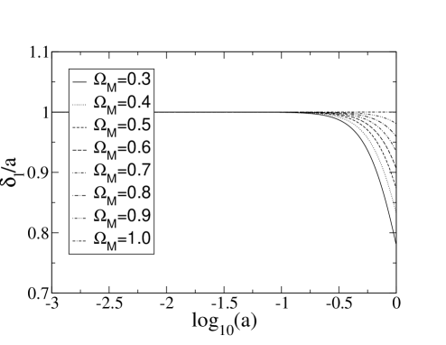
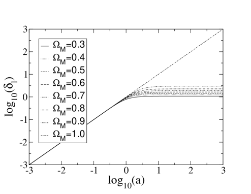
Figure 1: Linear growth with for different values of $\Omega_{M}$

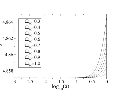
Figure 2: Non-linear growth for different values of $\Omega_{M}$

We see that the effect on the linear growth factor is significant as perturbations grow less when the cosmological constant is large compared to the energy density of matter. The effect of the cosmological constant on linear growth is well represented by the other figure where future evolution is shown. With a non-zero $\Omega_{\Lambda}$, $\delta_{l}$ freezes and structures stop growing in the future.

The effect on $S_{3}$ is very small, as expected, so that even when $\Omega_{M}=0.3$, $\Delta S_{3}<1\%$. Such a small change is clearly out of reach of present day observations as is discussed in more detail in Section 6.

3.2 Gravitational growth with a general Friedmann equation

In a general case with the Raychaudhuri’s equation given by Eq. (27), the equation governing large scale structure growth in the matter dominated universe can be derived following similar steps like in the standard case. The result is

$$\mbox{$$}{d^{2}\delta\over d\eta^{2}}+(2+{\dot{\overline{H}}\over\overline{H}^{2}}){d\delta\over d\eta}-\frac{4}{3}{1\over 1+\delta}({d\delta\over d\tau})^{2}=-3{1+\delta\over\overline{H}^{2}}\Big{(}(\dot{H}+H^{2})-(\dot{\overline{H}}+\overline{H}^{2})\Big{)},$$ (50)

where again $\eta=\ln(a)$. Obviously one cannot progress further unless the continuity equation is known so that $\dot{H}$ can be calculated. With the continuity equation one can then express $\rho$ in terms of $\bar{\rho}$ and $\delta$ using Eq. (36). The resulting equation can be expressed in terms of cosmological quantities, $\Omega_{M},\ \Omega_{\Lambda},$…, by writing the Friedmann equation in terms of $\Omega$s and noting that from Eq. (6) we get

$$\mbox{$$}\bar{\rho}={H_{0}^{2}\over\kappa^{2}a^{3}}\Omega_{M}.$$ (51)

We then have an equation determining the growth of density fluctuations, $\delta$, in terms of $\Omega$s. We can expand the $\dot{H}+H^{2}$-term in terms of $\delta$ and then the whole RHS of Eq. (50) as

$$\mbox{$$}3{1+\delta\over\overline{H}^{2}}\Big{(}(\dot{H}+H^{2})-(\dot{\overline{H}}+\overline{H}^{2})\Big{)}\equiv 3(1+\delta)\sum_{n=1}c_{n}\delta^{n}.$$ (52)

Note that there is no constant term in the expansion.

Expanding the perturbation according to Eq. (41) the linear equation is then

$$\mbox{$$}D_{1}^{\prime\prime}+(2+{\dot{\overline{H}}\over\overline{H}^{2}})D_{1}^{\prime}+3c_{1}D_{1}=0,$$ (53)

the second order equation

$$\mbox{$$}D_{2}^{\prime\prime}+(2+{\dot{\overline{H}}\over\overline{H}^{2}})D_{2}^{\prime}-\frac{8}{3}(D_{1}^{\prime})^{2}+3c_{1}D_{2}+6(c_{1}+c_{2})D_{1}^{2}=0$$ (54)

and further orders are easily found. For example, in the standard case we see that

$$\mbox{$$}c_{1} = -\frac{1}{2}{\kappa^{2}\overline{\rho}_{M}\over\overline{H}^{2}}=-\frac{1}{2}{\Omega_{M}\over\Omega_{M}+a^{3}\Omega_{\Lambda}}$$ (55)

$$c_{i} = 0,\ i=2,3,....$$ (56)

Using these, the linear and second order equations, Eqs (42) and (45) are easily reproduced.

Note that these expressions make only sense on large scales where the non-standard evolution of the universe can be seen. On small scales the evolution obviously must be according to the standard Einstein’s equations.

4 DGP

As we have seen, the two equations that determine how density perturbations grow are the Friedmann equation and the continuity equation. In the DGP- scenario these are:

$$\mbox{$$}0 = \dot{\rho}+3H(\rho+p)$$ (57)

$$H^{2} = H_{0}^{2}\Big{(}{\Omega_{M}\over a^{3}}+\Omega_{R}(2+\sqrt{1+{\Omega_{M}\over\Omega_{R}a^{3}}})\Big{)}.$$ (58)

In the DGP-case we cannot use Eq. (30) since the Einstein’s equations on the brane are modified from the standard four-dimensional equations as is apparent from the non-standard Friedmann equation. Another way of seeing the same thing is to consider in the DGP scenario the quantity appearing on the RHS of the Raychaudhuri’s equation, Eq. (26),

$$\mbox{$$}\dot{H}+H^{2}=-\frac{3}{2}\kappa^{2}(1+{1\over R\sqrt{\kappa^{2}\rho+{1\over R^{2}}}})(\rho+p)+\kappa^{2}\rho+{2\over R}\sqrt{\kappa^{2}\rho+{1\over R^{2}}}+{2\over R^{2}}.$$ (59)

This is different from the result that one gets in the standard case, $-\frac{3}{2}\kappa^{2}(\rho+3p)$, with the standard Einstein’s equations. In the DGP-scenario the Raychaudhuri’s equation hence needs to be calculated directly using the general approach described in the previous subsection.

In the matter dominated DPG-scenario:

$$\mbox{$$}{1\over H^{2}}(\dot{H}+H^{2})=\frac{\Omega_{M}\,\left({\sqrt{\Omega_{R}}}-{\sqrt{\frac{\Omega_{M}}{a^{3}}+\Omega_{R}}}\right)+4\,a^{3}\,\Omega_{R}\,\left({\sqrt{\Omega_{R}}}+{\sqrt{\frac{\Omega_{M}}{a^{3}}+\Omega_{R}}}\right)}{2\,a^{3}\,{\sqrt{\frac{\Omega_{M}}{a^{3}}+\Omega_{R}}}\,{\left({\sqrt{\Omega_{R}}}+{\sqrt{\frac{\Omega_{M}}{a^{3}}+\Omega_{R}}}\right)}^{2}}.$$ (60)

The coefficients $c_{i}$ are easily calculated and the first two are, again expressed in cosmological quantities:

$$\mbox{$$}c_{1} = -\frac{2\,\left(\Omega_{M}+\Omega_{R}\,{a}^{3}\right)\,\left(\Omega_{M}+4\,\Omega_{R}\,{a}^{3}\right)+{\sqrt{\Omega_{R}}}\,{\sqrt{\Omega_{R}+\frac{\Omega_{M}}{{a}^{3}}}}\,{a}^{3}\,\left(5\,\Omega_{M}+8\,\Omega_{R}\,{a}^{3}\right)}{4{\left(\Omega_{M}+\Omega_{R}\,{a}^{3}\right)}^{2}}$$

$$c_{2} = \frac{\Omega_{M}^{2}\,{\sqrt{\Omega_{R}}}\,{\sqrt{\Omega_{R}+\frac{\Omega_{M}}{{a}^{3}}}}\,\left(8\Omega_{R}\,a^{3}-\Omega_{M}\right)}{16\,{\left({\sqrt{\Omega_{R}}}+{\sqrt{\Omega_{R}+\frac{\Omega_{M}}{{a}^{3}}}}\right)}^{2}\,{\left(\Omega_{M}+\Omega_{R}\,{a}^{3}\right)}^{3}}.$$

Finally, we need to calculate the term appearing in front of the $\delta^{\prime}$-term in the perturbation equation (50):

$$\mbox{$$}2+{\dot{H}\over H^{2}}=\frac{1}{2}+\frac{3\,{\sqrt{\Omega_{R}}}}{2\,{\sqrt{\Omega_{R}+\frac{\Omega_{M}}{{a}^{3}}}}}.$$ (61)

Clearly, in the limit $\Omega_{R}=0$, all these expressions reduce to the corresponding expressions in the Einstein-deSitter case.

We can now study the growth of perturbations numerically. The initial conditions are chosen such that at $a=10^{-3}$, the standard exponential solution, $D_{1}\sim\exp(\eta)$, is reached. In calculating the second order perturbation, initial conditions are chosen such that the standard solution, constant $S_{3}=\frac{34}{7}\approx 4.86$ is valid from the beginning. In Fig. 3 the linear growth factor (and the linear growth factor normalized with the scale factor) for different values of $\Omega_{R}$, with $\Omega_{M}$ then determined by Eq. (10), are shown as a function of the scale factor. The non-linear growth is shown in Fig. 4.

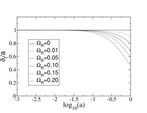
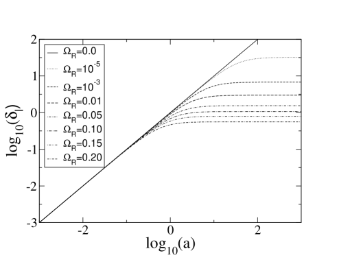
Figure 3: Linear growth for different values of $\Omega_{R}$

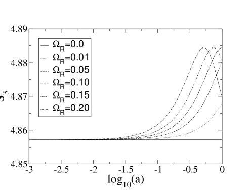
Figure 4: Non-linear growth for different values of $\Omega_{R}$

The general form of the linear growth factor is similar to the cosmological constant case but here the effect is even more pronounced. For the preferred value $\Omega_{R}=0.17$ Dvali et al. (2000), the growth of linear fluctuations up to now is suppressed by a factor of $0.54$ compared to the EdS-case. In the $\Lambda$-universe with $\Omega_{\Lambda}=0.7$, the suppression is $0.78$. Hence, there will be significantly less structure growth on large scales in the DGP-scenario than in a $\Lambda$-cosmology. Furthermore, the suppression begins earlier in the DGP-scenario as is visible from Fig. 4.

The second order perturbation, or $S_{3}$, also grows differently from the $\Lambda$-cosmology. The value of $S_{3}$ starts to grow at earlier times and varies more than in the standard $\Lambda$-universe. However, the variation is still observationally insignificant being at best less than one percent.

5 Cardassian models

In this section will consider the growth of gravitational instabilities in the Modified Polytropic Cardassian model described by Eq. (19). The relevant equations in a matter dominated universe are

$$\mbox{$$}0 = \dot{\rho}+3H\rho$$ (62)

$$H^{2} = \kappa^{2}\,\rho{\Big{(}1+(1+{z_{eq}})^{3(1-n)q}(\frac{\rho}{{\rho_{0}}})^{(n-1)q}\Big{)}}^{\frac{1}{q}}$$ (63)

From these all the relevant quantities can be calculated straightforwardly.

The $\dot{H}+H^{2}$-term is

$$\mbox{$$}{1\over H^{2}}(\dot{H}+H^{2})=-\frac{1}{2}\frac{1+(1+z_{eq})^{3(1-n)q}(3n-2)(\frac{\rho}{\rho_{0}})^{(n-1)q}}{1+(1+z_{eq})^{3(1-n)q}(\frac{\rho}{\rho_{0}})^{(n-1)q}}$$ (64)

and the first two $c_{i}$ coefficients

$$\mbox{$$}c_{1} = -\frac{1}{2}\frac{1+(4n-2+3(n-1)^{2}q)X+n(3n-2)X^{2}}{\Big{(}1+X\Big{)}^{2}}$$ (65)

$$c_{2} = \frac{X}{4}(1+X)^{-3}(n-1)\Big{[}\Big{(}(1-n)q-1\Big{)}\Big{(}1+3(n-1)q\Big{)}$$ (67)

$$+\Big{(}2-4n-(n-1)(9n-5)q+3(n-1)^{2}q^{2}\Big{)}X+n(2-3n)X^{2}\Big{]},$$

where we have defined $X\equiv((1+z_{eq})a)^{3(1-n)q}$ in order to shorten the otherwise lengthy expressions.

In the original Cardassian case with q=1, these expressions simplify to

$$\mbox{$$}c_{1} = {-\frac{1}{2}+n(1-\frac{3}{2}n)(1+z_{eq})^{3(1-n)}a^{3(1-n)}\over 1+(1+z_{eq})^{3(1-n)}a^{3(1-n)}}$$ (68)

$$c_{2} = {\frac{1}{2}n(n-1)(1-\frac{3}{2}n)(1+z_{eq})^{3(1-n)}a^{3(1-n)}\over 1+(1+z_{eq})^{3(1-n)}a^{3(1-n)}}.$$ (69)

Again, as a check it is easy to see that with $n=0$, we recover the standard coefficients (55).

Finally, in order to study the growth of perturbations, we need the coefficient of the $\delta^{\prime}$ term:

$$\mbox{$$}2+{\dot{\overline{H}}\over H^{2}}=2-\frac{3}{2}{1+n(1+z_{eq})^{3q(1-n)}a^{3q(1-n)}\over 1+(1+z_{eq})^{3q(1-n)}a^{3q(1-n)}}.$$ (70)

We can now calculate the growth of perturbations in the original Cardassian scenario. Initial conditions are chosen like in the DGP scenario.

The solution to the linear equation in the original Cardassian model can be expressed in terms of the hypergeometric function. The growing part of the solution is found to be

$$\mbox{$$}D_{1}(x)=e^{x}\,\;F_{1{\hskip-16.0pt}2}{\hskip 11.0pt}\Big{[}1,\frac{2+3n}{6(1-n)},{11-6n\over 6(1-n)},-e^{3(1-n)x}\Big{]},\ n<\frac{2}{3}.$$ (71)

For the general case, no such solution is found.

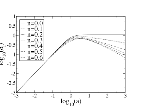
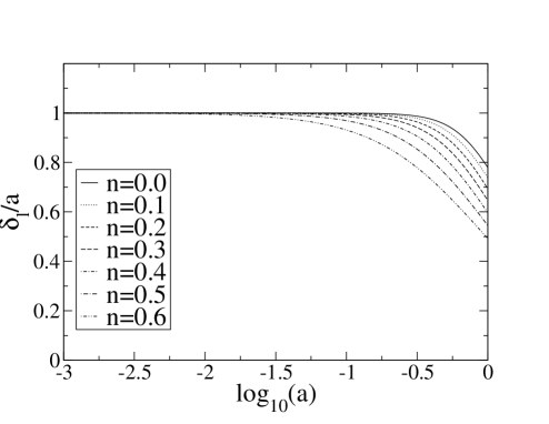
Figure 5: Linear growth for different values of $n$, $q=1$

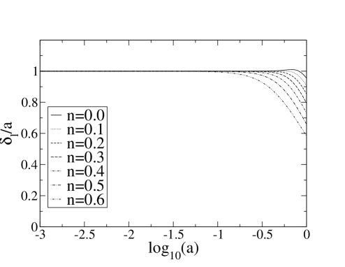
Figure 6: Linear growth for different values of $n$, $q=2$

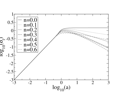
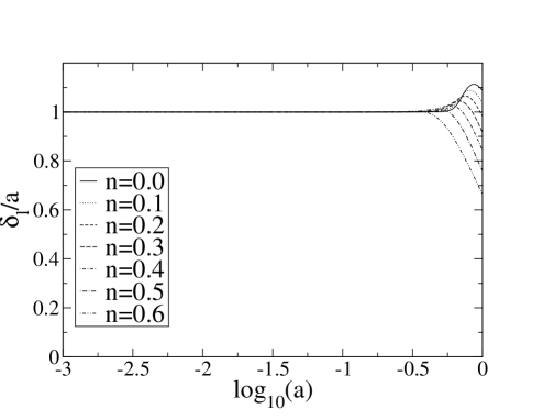
Figure 7: Linear growth for different values of $n$, $q=5$

Figure 8: Linear growth for different values of $n$, $q=10$.

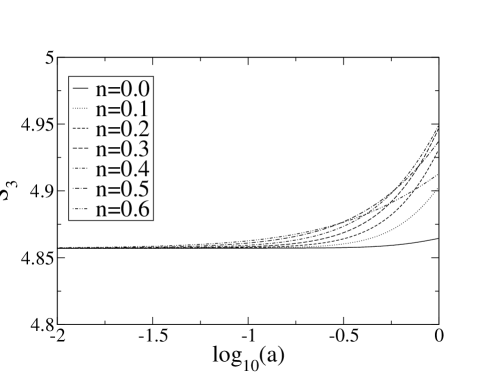
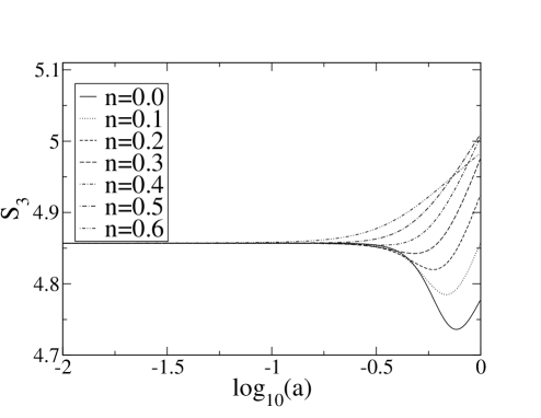
Figure 9: Non-linear growth for different values of $n$, $q=1,\ 2$.

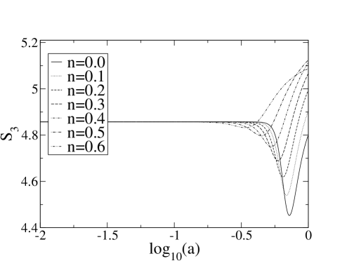
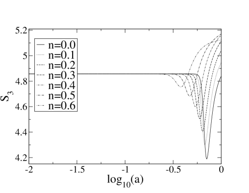
Figure 10: Non-linear growth for different values of $n$, $q=5,\ 10$.

We have plotted the linear and non-linear growth factors for $n=0,0.1,...,0.6$ and $q=1,2,5,10$ as a function of $a$ in Figs 5-10. The linear growth factor is presented both on a logarithmic scale and scaled by the scale factor. In plotting these figures, we have assumed that $\Omega_{M}^{obs}=0.3$, which then sets the value of $z_{eq}$ according to Eq. (21).

From the figures it is clear how the Cardassian scenario is fundamentally different from the DGP-model and a $\Lambda$-cosmology. Looking at the behavior of $\delta_{l}$ with $n>0$ (since $n=0$ corresponds to a cosmological constant) the linear growth factor actually begins to decrease in the future i.e. areas of higher density begin to rarify. This is true regardless of the value of $q$. Near the turning point there is some interesting behavior as is visible from the plots of $\delta_{l}/a$. With larger values of $q$ we see that before the growth factor starts to decrease, structures grow more rapidly compared to the standard case. This was not seen in neither of the other models studied in this paper. The value of $\delta_{l}/a$ at present is dependent on the value of the parameters but can again be as small as $0.5$.

In Fig. 5 $q=1$ and we are hence looking at the original Cardassian model. This is of interest since in this case we can understand some of the features by analytical considerations. For example, we see that the value of $n$ that corresponds to the slowest growth is $n\approx 0.4$. If one considers the equation determining linear growth in more detail, it can be seen that in the limit $a\rightarrow\infty$, the slowest growth actually corresponds to $n=\frac{4}{9}$ with $D_{1}(a)\sim a^{-\frac{2}{3}}$ as is shown in the Appendix.

Looking at the figures depicting the change in $S_{3}$, Figs 9 and 10, we see that in the Cardassian model the evolution of the value of $S_{3}$ is strongly dependent on the value of $q$. The shape and the magnitude of variation changes with $q$ so that with larger $q$ one sees larger variations.

In the original Cardassian scenario the values of $S_{3}$ grow compared to the EdS scenario. The overall shape of the curves is similar to that of the standard $\Lambda\neq 0$ universe described in Sec. 3.1. However, here the scale of the change in $S_{3}$ is much larger than in the standard $\Lambda\neq 0$ universe. The growth of non-linearities seems to be fastest for $n\approx 0.3$. Analytical considerations, see Appendix, show that in the large $a$ limit, the value of $n$ corresponding to fastest growth at large $a$ is again $n=\frac{4}{9}$. The magnitude of change in $S_{3}$ is approximately two percent with $n=0.3$, which, although larger than in the DGP-scenario or $\Lambda$-cosmology, is out of reach of present day experiments.

However, as $q$ is increased, also the variation of $S_{3}$ grows. For example, with $q=10$, we see that $S_{3}$ can vary more than $10$ percent from its EdS value. Also with $q\;\raise 1.29167pt\hbox{$>$\kern-7.5pt\raise-4.73611pt\hbox{$\sim$}}\;2$, the values of $S_{3}$ undergo a change from values smaller than $S_{3}^{EdS}$ to values larger than $S_{3}^{EdS}$.

6 Observational constraints

As mentioned in the introduction, the above non-standard models have been tested mostly against observations of SNIa and CMB. The analysis presented in this paper allows for a further comparison with constrains coming from linear and non-linear aspects of structure formation, i.e. : $\sigma_{8}$ normalization, cluster number density and skewness of the density field. The shape of the initial spectrum of fluctuations $P(k)$ as a function of wavenumber $k$, could also depend strongly on cosmological parameters (see eg Efstathiou, Sutherland & Maddox 1990). But this requieres additional ingredients to our models: ie knowledge of the primordial spectrum and the matter content. Here we concentrate only in aspects that relate to the matter dominated evolution, assuming some given initial shape $P(k)$. We briefly sketch how this comparison can be done and leave a more direct parameter estimation for future work.

6.1 Amplitude normalization: $\sigma_{8}$

The amplitude of density fluctuations is commonly characterized by the linear value of the rms fluctuations on a sphere of $8Mpc/h$. Observationally its value seems to be of order unity at $z=0$. Form the analysis in the previous sections it is straight forward to predict how different $\sigma_{8}$ should be for a given cosmological model. One way to do this is to fix the normalization of all models to be equal at high red-shifts and see how different they are at $z=0.5$. Figure 11 illustrates this point. We show the value of $\sigma_{8}$ normalized to the $\Lambda$ model as a function of red-shift for DGP and MPC ($n=0.6$ and $q=1$) cosmologies, all with same value of $\Omega_{m}=0.22$.

Figure 11: Value of $\sigma_{8}$ in non-standard cosmologies, with $\Omega_{M}=0.22$, relative to the value for the $\Omega_{\Lambda}=0.78$, $\Omega_{M}=0.22$ standard cosmology with $\sigma_{8}=1$.

Values of $\sigma_{8}$ for other parameters can readily be obtained by comparing Figure 1 with Figure 3 and Figures 5-8. Note how for MPC with $q>1$ we can also get $\sigma_{8}>1$.

Current observational constraints of $\sigma_{8}$ usually come with several different assumptions. In most cases a shape for the linear spectrum is assumed to get an estimation, for example from cluster abundances or normalization of CMB fluctuations. If the primordial spectrum of fluctuations is not scale invariance or a simple power-law, such extrapolations could yield misleading values of $\sigma_{8}$ (e.g. see Barriga et al. (2001) and references therein). Large scale structure in local galaxy catalogues also yield values $\sigma_{8}\simeq 1$, but one needs to quantify the bias $b$, or how well the selected galaxies trace the underlying mass distribution (see e.g. Gaztañaga 1995). Recent CMB results from the WMAP (Spergel et al. 2003) mission fit to the (power-law) $\Lambda$CDM cosmology find: $\sigma_{8}=0.9\pm 0.1$ ($\sigma_{8}=0.84\pm 0.04$ with a running index, Spergel et al. (2003)). This value has been extrapolated from $z\simeq 10^{3}$ to $z=0$ by using the linear growth factor $D_{1}(z)$ in Eq. (44). Significantly smaller values ($\sigma_{8}\simeq 0.6-0.7$) have been found at low red-shifts by weak lensing (see e.g. Jarvis et al. (2002)) and velocity fields (e.g. Willick & Strauss 1998). This apparent discrepancy, if real, could be easily accounted for by using the DGP or MPC cosmological models.

6.2 The number counts of galaxies

Figure 12: Bottom: Comoving volume element as a function of red-shift normalized to the EdS model. The short and long dashed line shows DGP and MPC predictions for $\Omega_{M}=0.22$ ($\Omega_{R}=0.15$) and $h=0.71$. The continuous line corresponds to the $\Lambda$ cosmology with $\Omega_{M}=0.22$ ($\Omega_{\Lambda}=0.78$) and $h=0.71$. Top: Number density of predicted clusters per square degree with mass $M>2\times 10^{14}M_{solar}$ for the same models. All models are normalized to $\sigma_{8}=1$ at $z=0$.

Press & Schechter formalism (Press & Schechter 1974) and its extensions (see e.g. Bond et al. 1991; Lacey & Cole 1993) predict the evolution of the mass function of collapse objects. These predictions are based on assuming Gaussian initial conditions and the spherical collapse model (which is closely related to the shear-free approximation used in Eq. (22)). Despite the apparent limitations of these assumptions, comparison with realistic simulations show good agreement (see a recent review by Cooray & Sheth (2002)). In the standard Press-Schechter formalism, the comoving number density of collapsed objects (halos or clusters) of mass $M$ is

$$n(M)dM=-\sqrt{2\over\pi}\,\left({\delta_{c}\over\sigma}\right){d\ln\sigma\over d\ln M}\,\exp{\left(-{\delta_{c}^{2}\over 2\sigma^{2}}\right)}\,{\bar{\rho}\,dM\over M^{2}}$$ (72)

where $\sigma=\sigma(R,z)$ is the linear rms fluctuation at the scale $R$ corresponding to the mass $M=4/3\pi R^{3}\bar{\rho}$, and $\bar{\rho}$ is the mean background. The value of $\delta_{c}$ corresponds to the value of the linear over-density at the time of collapse, i.e. when the non-linear over-density becomes very large $\delta\rightarrow\infty$. This value can be found by solving Eq.(37). For the standard Einstein-de Sitter case we have $\delta_{c}\simeq 1.686$. We find little difference in $\delta_{c}$ for the non-standard cosmologies, so for simplicity we will use the EdS value in all cases.

To translate the above predictions into observable quantities, such as the number density of clusters per unit red-shift, above a certain mass, we need to integrate over the comoving volume element $dV/dz$, which is also a strong function of the cosmology. Bottom panel of Figure 12 shows the comoving volume element (normalized to EdS case) in the DGP (dashed line), MPC (long dashed line) and $\Lambda$ cosmology (continuous line). As can be seen in the figure, the $\Lambda$ cosmology has about 4 times more comoving volume by $z\simeq 1.5$ than the EdS case, while DGP and MPC are only 3 and 2 times larger. Despite the smaller volumes, DGP and MPC predicts 2 and 4 times more clusters at $z\simeq 1.5$ than the $\Lambda$ cosmology because of the stronger freeze in the linear growth factor, which can be seem by comparing Figure 1 to Figure 3.

Note that there are four important factors in the PS predictions: i) $\Omega_{M}$, which relates a given cluster mass $M$ to $R$ in $\sigma(R)$ value, ii) the shape of the power spectrum, which determines the $\sigma(R)$ curve, iii) the volume element, and iv) the growth factor $D_{1}(z)$ which gives the red-shift variation of $\sigma$. In our analysis we fixed i) and ii) to the $\Lambda$ cosmology with $\Omega_{M}\simeq 0.22$. Thus all differences in Figure 12 are due to differences in volume and growth factors, which mark the distinction between standard and non-standard cosmologies.

6.3 The skewness $S_{3}$

We have already shown the predictions for the normalized skewness, $S_{3}$ in Eq. (47), in Figures 2, 4, 9 and 10 (see also Eq. (80) in the appendix). These are the unsmoothed values of the skewness at a single point. In practice, to relate to observations, one needs to take into account smoothing effects. For a top-hat window of a given radius $R$, smoothing results in a simple linear correction that is given by the slope $\gamma$ of the variance smoothed at a radius $R$ (Juskiewicz, Bouchet & Colombi 1993). In the standard cosmology: $S_{3}=34/7+\gamma$ (eg see Bernardeau et al. (2002) and references therein). The smoothing correction should be the same for non-standard cosmologies, as long as we work within the spherical collapse model (ie the shear-free approximation in Eq. (22)), which gives the exact leading order contribution to $S_{3}$ for a top hat window (see e.g. Fosalba & Gaztañaga 1998; Bernardeau et al. 2002). Thus, the difference between the standard predictions and the predictions from non-standard cosmologies should not be affected by these smoothing effects. Besides smoothing effects, $S_{3}$ is also affected by systematic uncertainties of biasing (see §7.1 in Bernardeau et al. 2002).

Current estimations for $S_{3}$ (see §8 in Bernardeau et al. (2002)) agree with the standard predictions but with large uncertainties, of order $20\%-30\%$. Thus current observations on $S_{3}$ can not be used to separate the different models. Next generation catalogues, such as the Sloan Digital Sky Survey, are expected to reduce the sampling variance uncertainties to $5\%$ (see e.g. Szapudi, Colombi & Bernardeau 1999; Verde et al. 2000). Thus, after removing biasing uncertainties, future measurements on $S_{3}$ could be used to constraint some of the MPC parameters (e.g. see Figs. 9 and 10).

7 Conclusions

In this paper we have studied the growth of large scale structure in non-standard cosmological scenarios that can undergo acceleration without having an explicit cosmological constant. In order to do this, we have extended the standard spherical collapse formalism to account for the non-standard equations. All that is needed is the Friedmann equation and the assumption that the energy density of matter is conserved. The applicability of our approach is limited to very large scales, where Einstein’s equations can be modified. Of the two studied scenarios, the DGP-model is more attractive since it is based on physics coming from brane cosmology whereas the MPC-model is a more phenomenological approach. In a flat universe the DGP-model has only a single free parameter, $\Omega_{M}$, but this model is still found to be in accordance with the current observations on large scale structure. The MPC model has two additional parameters so that it is less surprising that observations on large scale structure do not rule out such a model.

In the DGP- and MPC- models it was found that linear growth is inhibited due to the accelerated expansion, like in the standard $\Lambda$-cosmology. Depending on the values of the parameters, the suppression at present compared to the EdS-case can be as much as 50%. The non-linear growth was studied by considering the value of the skewness. For DGP, the deviation from the EdS-value is larger than in the $\Lambda$-case but still only of the order of one percent. In the MPC-scenario, however, the story is quite different and the value of skewness can vary up to $10$ percent.

In order to evaluate the significance of the non-standard evolution of large scale perturbations, one obviously needs to relate the predictions of the linear and non-linear growth rate to observations. As was discussed in Section 6, the linear normalization of large scale density fields can vary greatly. The value of $\sigma_{8}$ can be much smaller in the MPC- and DGP- scenarios when compared to the standard $\Lambda$-cosmology with the same normalization at high redshift. Intriguingly, there is already some observational indication of a small value of $\sigma_{8}$ at low red-shifts but more observational data is needed in order to determine whether this effect is real. We also find that in the MPC-scenario, the linear growth can actually be faster than in the EdS universe for a limited range of red-shift. This is an interesting property since models that have late time acceleration typically lead to less linear growth at all times. In any case, observations of $\sigma_{8}$ at low red-shifts, combined with the precision CMB data coming from the WMAP (and in the future Planck) mission, will be a powerful probe of non-standard cosmological evolution.

Another quantity that is strongly affected by the non-standard linear evolution is the number counts of objects. As it was shown in Section 6, using the Press-Schechter formalism gives strong predictions for the number of clusters that differ significantly from one expects in a $\Lambda$-cosmology. Again, studying the number counts of clusters at different red-shifts gives another way to constrain non-standard cosmological models such as the DGP- and MPC-scenarios.

The higher order statistics can also be modified by the non-standard effects. In this paper we have considered the normalized skewness, $S_{3}$, whose evolution can be straightforwardly extracted in each model. The skewness gives another probe of possible atypical cosmological evolution. Typically, the effect on the skewness of different cosmological scenarios, e.g. $\Lambda$-cosmology and quintessence Benabed & Bernardeau (2001), is very small and totally unobservable. However, as we have seen here (see also Gaztañaga & Lobo 2001), the effect can be much larger and can possibly be detected in the near future experiments such as the Sloan Digital Sky Survey.

The growth of large scale structure is tightly bound to the overall evolution of the universe and hence to the particular cosmological model. As such, along with the SNIa and CMB data, it is a powerful tool to probe the space of possible cosmologies. Current large scale structure data agrees well with the two proposals that explain late time acceleration without a cosmological constant. This agreement is not trivial in the case of DGP, as there are no additional free parameters, once we fit to the SNIa data or the value of $\Omega_{M}$. We have shown here how upcoming surveys of large scale structure can be used to further constrain these non-standard models and differentiate then from the now standard $\Lambda$ model.

Appendix A Growth of linear and second order perturbations in the Cardassian model

In this appendix, we consider the growth of linear and second order fluctuations in the original Cardassian model, $q=1$, by analytical means.

A.1 Linear growth

The equation determining linear growth, Eq. (53), in the Cardassian model in a scaled form is

$$\mbox{$$}{d^{2}D_{1}\over dx^{2}}+\Big{(}2-\frac{3}{2}{1+ne^{3(1-n)x}\over 1+e^{3(1-n)x}}\Big{)}{dD_{1}\over dx}+\frac{3}{2}{2n(1-\frac{3}{2}n)e^{3(1-n)x}-1\over e^{3(1-n)x}+1}D_{1}=0,$$ (73)

where $x\equiv\ln(a/a_{C})=\eta-\eta_{C}$.

It is now interesting to look at the large $\left|x\right|$ limits. Since we are interested in the range of values where $0<n<\frac{2}{3}$, it is clear that at, depending on the sign of $x$, the exponential terms in Eq. (73) will either dominate or be negligible in the large $x$ limit. When $x$ is large and negative, i.e. when $a/a_{C}\ll 1$, Eq. (73) takes the form

$$\mbox{$$}{d^{2}D_{1}\over dx^{2}}+{1\over 2}{dD_{1}\over dx}-\frac{3}{2}D_{1}=0,$$ (74)

i.e. the standard form, which has the usual solution

$$\mbox{$$}D_{1}^{-}(x)=A_{1}e^{x}+A_{2}e^{-\frac{3}{2}x}.$$ (75)

In the large positive $x$-limit, i.e. when $a/a_{C}\gg 1$, it is obvious that the exponential terms will dominate and so that Eq. (73) can be written as

$$\mbox{$$}{d^{2}D_{1}\over dx^{2}}+(2-\frac{3}{2}n){dD_{1}\over dx}+3n(1-\frac{3}{2}n)D_{1}=0.$$ (76)

The solution to this equation is easily found and reads as

$$\mbox{$$}D_{1}^{+}(x)=B_{1}e^{-\frac{3}{2}nx}+B_{2}e^{(3n-2)x},$$ (77)

where $B_{i}$ are constants. Looking at the solutions, we see that with $n=1$, the two solutions agree as expected. If $n<\frac{2}{3}$, the linear growth of perturbations will at some point stop and perturbations start to shrink.

The slowest growth rate at large $a/a_{C}$ is easily deduced from $D_{1}^{+}(x)$ and occurs when $-\frac{3}{2}n=3n-2$ i.e. when $n=\frac{4}{9}$ and hence $D_{1}^{+}(x)\sim e^{-\frac{2}{3}x}$.

A.2 Second order perturbations

The equation determining the growth of second order perturbations in the large $x$ limit, in the negative large $x$ limit we obviously reproduce the standard scenario again, is from Eq. (54),

$$\mbox{$$}{d^{2}D_{2}\over dx^{2}}+(2-\frac{3}{2}n){dD_{2}\over dx}+3n(1-\frac{3}{2}n)D_{2}-\frac{8}{3}\Big{(}{dD_{1}\over dx})^{2}+3n(n+1)(1-\frac{3}{2}n)D_{1}^{2}=0.$$ (78)

The part that will dominate the linear solution $D_{1}$ depends on $n$, if $n<\frac{4}{9}$, $D_{1}\sim\exp(-\frac{3}{2}nx)$, where as if $\frac{4}{9}<n<1$, $D_{1}\sim\exp((3n-2)x)$. Let us first assume that $n<\frac{4}{9}$, in which case by substituting the appropriate solution of $D_{1}$ into Eq. (78) and solving the resulting equation, we get

$$\mbox{$$}D_{2}(x)=\frac{1}{2}(2+n)e^{-3nx}+C_{1}e^{-\frac{3}{2}nx}+C_{2}e^{(3n-2)x}.$$ (79)

Hence, since $n<\frac{4}{9}$, we see that in the large $x$ limit, $D_{2}\sim e^{-\frac{3}{2}nx}$. Therefore, we expect that in this limit,

$$\mbox{$$}S_{3}\sim e^{\frac{3}{2}nx}.$$ (80)

If we instead look at the values of $\frac{4}{9}<n<1$, we see that $S_{3}\sim e^{(2-3n)x}$, and hence the value of $n$ that gives the largest effect rate of change of $S_{3}$ is, again, at $n=\frac{4}{9}$ with $S_{3}\sim e^{\frac{2}{3}x}$.

References

- (1) Avelino P.P., Martins C.J.A.P., 2002, ApJ, 565, 661
- Barriga et al. (2001) Barriga J., Gaztañaga E., Santos M., Sarkar S., 2001, MNRAS, 324, 977
- Benabed & Bernardeau (2001) Benabed K., Bernardeau F., 2001, Phys. Rev., D64, 083501
- Bernardeau et al. (2002) Bernardeau F., Colombi S., Gaztañaga E., Scoccimarro R., 2002, Phys. Rep., 367, 1
- (5) Bond J.R., et al., 1991, ApJ, 379, 440
- (6) Chung D.J., Freese K., 2000, Phys. Rev., D61, 023511
- (7) Cline J., Vinet J., 2002, preprint (hep-ph/0211284)
- (8) Cooray A., Sheth R., 2002, Phys. Rep., 372, 1
- Dvali et al. (2000) Dvali G., Gabadadze G., Porrati M., 2000, Phys. Lett., B485, 208
- (10) Deffayet C., Landau S.J., Raux J., Zaldarriaga M., Astier P., 2002a, Phys. Rev., D66, 024019
- (11) Deffayet C., Dvali G., Gabadadze G., 2002b, Phys. Rev., D65, 044023
- (12) Dvali G., Gruzinov A., Zaldarriaga M., 2002, preprint (hep-ph/0212069)
- (13) Efstathiou, G., Maddox, S.J., Sutherland, W.J., 1990, Nature, 348, 705
- (14) Fosalba P., Gaztañaga E., 1998, MNRAS, 301, 503
- (15) Freese K., 2002, preprint (hep-ph/0208264)
- (16) Freese K., Lewis M., 2002, Phys. Lett., B540, 1
- (17) Gaztañaga E., 1995, ApJ, 454, 561
- (18) Gaztañaga E., Lobo J.A., 2001, ApJ, 548, 47
- (19) Gondolo P., Freese K., 2002, preprint (hep-ph/0209322)
- Jarvis et al. (2002) Jarvis M., Bernstein G., Jain B., Fischer P., Smith D., Tyson J.A., Wittman D., 2002, preprint (astro-ph/0210604)
- (21) Juszkiewicz, R., Bouchet, F.R., Colombi, S., 1993, ApJ, 412, L9
- (22) Lacey C., Cole S., 1993, MNRAS, 262, 627
- (23) Lue A., Starkman G., 2002, preprint (astro-ph/0212083)
- (24) Peebles P.J.E., Principles of Physical Cosmology, Princeton, 1993
- (25) Perlmutter S. et al., 1999, ApJ, 517, 565
- (26) Press W.H., Schechter P., 1974, ApJ, 187, 425
- (27) Riess A.G. et al., 1998, AJ, 116, 1009
- (28) Sen S., Sen A.A., 2002, preprint (astro-ph/0211634)
- (29) Sen S., Sen A.A., 2003, preprint (astro-ph/0303383)
- Spergel et al. (2003) Spergel D.N. et al., 2003, preprint (astro-ph/0302209)
- (31) Szapudi I., Colombi S., Bernardeau F., 1999, MNRAS, 310, 428
- (32) Verde L., Wang L., Heavens A.F., Kamionkowski M., 2000, MNRAS, 313, 141
- (33) Wang Y., Freese K., Gondolo P., Lewis M., 2003, preprint (astro-ph/0302064)
- (34) Weinberg S., 1989, Rev. Mod. Phys., 61, 1
- (35) Willick J.A., Strauss M.A., 1998, ApJ, 507, 64
- (36) Zhu Z., Fujimoto M., 2002, ApJ, 581, 1
- (37) Zhu Z., Fujimoto M., 2003, preprint (astro-ph/0303021)