Populating Dark Matter Haloes with Galaxies: Comparing the 2dFGRS with Mock Galaxy Redshift Surveys

Abstract

In two recent papers, we developed a powerful technique to link the distribution of galaxies to that of dark matter haloes by considering halo occupation numbers as function of galaxy luminosity and type. In this paper we use these distribution functions to populate dark matter haloes in high-resolution $N$-body simulations of the standard $\Lambda$CDM cosmogony with $\Omega_{m}=0.3$, $\Omega_{\Lambda}=0.7$, and $\sigma_{8}=0.9$. Stacking simulation boxes of $100h^{-1}\>{\rm Mpc}$ and $300h^{-1}\>{\rm Mpc}$ with $512^{3}$ particles each we construct Mock Galaxy Redshift Surveys out to a redshift of $z=0.2$ with a numerical resolution that guarantees completeness down to $0.01L^{*}$. We use these mock surveys to investigate various clustering statistics. The predicted two-dimensional correlation function $\xi(r_{p},\pi)$ reveals clear signatures of redshift space distortions. The projected correlation functions for galaxies with different luminosities and types, derived from $\xi(r_{p},\pi)$, match the observations well on scales larger than $\sim 3\>h^{-1}{\rm{Mpc}}$. On smaller scales, however, the model overpredicts the clustering power by about a factor two. Modeling the “finger-of-God” effect on small scales reveals that the standard $\Lambda$CDM model predicts pairwise velocity dispersions (PVD) that are $\sim 400\>{\rm km}\,{\rm s}^{-1}$ too high at projected pair separations of $\sim 1h^{-1}\>{\rm Mpc}$. A strong velocity bias in massive haloes, with $b_{\rm vel}\equiv\sigma_{\rm gal}/\sigma_{\rm dm}\sim 0.6$ (where $\sigma_{\rm gal}$ and $\sigma_{\rm dm}$ are the velocity dispersions of galaxies and dark matter particles, respectively) can reduce the predicted PVD to the observed level, but does not help to resolve the over-prediction of clustering power on small scales. Consistent results can be obtained within the standard $\Lambda$CDM model only when the average mass-to-light ratio of clusters is of the order of $1000\>({\rm M}/{\rm L})_{\odot}$ in the $B$-band. Alternatively, as we show by a simple approximation, a $\Lambda$CDM model with $\sigma_{8}\simeq 0.75$ may also reproduce the observational results. We discuss our results in light of the recent WMAP results and the constraints on $\sigma_{8}$ obtained independently from other observations.

1 Introduction

The distribution of galaxies contains important information about the large scale structure of the matter distribution. On large, linear scales the galaxy power spectrum is believed to be proportional to the matter power spectrum, therewith providing useful information regarding the initial conditions of structure formation, i.e., regarding the power spectrum of primordial density fluctuations. On smaller, non-linear scales the distribution and motion of galaxies is governed by the local gravitational potential, which is cosmology dependent. One of the main goals of large galaxy redshift surveys is therefore to map the distribution of galaxies as accurately as possible, over as large a volume as possible. The Sloan Digital Sky Survey (SDSS; York et al. 2000) and the 2 degree Field Galaxy Redshift Survey (2dFGRS; Colless et al. 2001) are two of the prime examples. These surveys, which are currently being completed, will greatly enhance and improve our knowledge of large-scale structure and will become the standard data sets against which to test our cosmological and galaxy formation models for the decade to come.

However, two effects complicate a straightforward interpretation of the data. First of all, the distribution of galaxies is likely to be biased with respect to the underlying mass density distribution. This bias is an imprint of various complicated physical processes related to galaxy formation such as gas cooling, star formation, merging, tidal stripping and heating, and a variety of feedback processes. In fact, it is expected that the bias depends on scale, redshift, galaxy type, galaxy luminosity, etc. (Kauffmann, Nusser & Steinmetz 1997; Jing, Mo & Börner 1998; Somerville et al. 2001; van den Bosch, Yang & Mo 2003). Therefore, in order to translate the observed clustering of galaxies into a measure for the clustering of (dark) matter, one needs to either understand galaxy formation in detail, or use an alternative method to describe the relationship between galaxies and dark matter (haloes). One of the main goals of this paper is to advocate one such method and to show its potential strength for advancing our understanding of large scale structure.

Secondly, because of the peculiar velocities of galaxies, the clustering of galaxies observed in redshift-space is distorted with respect to the real-space clustering (e.g., Davis & Peebles 1983; Kaiser 1987; Regos & Geller 1991; van de Weygaert & van Kampen 1993; Hamilton 1992). On small scales, the virialized motion of galaxies within dark matter haloes smears out structure along the line-of-sight (i.e., the so-called “finger-of-God” effect). On large scales, coherent flows induced by the gravitational action of large scale structure enhance structure along the line-of-sight. Both effects cause an anisotropy in the two-dimensional, two-point correlation function $\xi(r_{p},\pi)$, with $r_{p}$ and $\pi$ the pair separations perpendicular and parallel to the line-of-sight, respectively. The large-scale flows compress the contours of $\xi(r_{p},\pi)$ in the $\pi$ direction by an amount that depends on $\beta\equiv\Omega_{m}^{0.6}/b$. The small-scale peculiar motions implies that $\xi(r_{p},\pi)$ is convolved in the $\pi$-direction by the distribution of pairwise velocities, $f(v_{12})$. Thus, the detailed structure of $\xi(r_{p},\pi)$ contains information regarding the Universal matter density $\Omega_{m}$, the (linear) bias of galaxies $b$, and the pairwise velocity distribution $f(v_{12})$.

From the above discussion it is obvious that understanding galaxy bias is an integral part of understanding large scale structure. One way to address galaxy bias without a detailed theory for how galaxies form is to model halo occupation statistics. One simply specifies halo occupation numbers, $\langle N(M)\rangle$, which describe how many galaxies on average occupy a halo of mass $M$. Many recent investigations have used such halo occupation models to study various aspects of galaxy clustering (Jing, Mo & Börner 1998; Peacock & Smith 2000; Seljak 2000; Scoccimarro et al. 2001; White 2001; Jing, Börner & Suto 2002; Bullock, Wechsler & Somerville 2002; Berlind & Weinberg 2002; Scranton 2002; Kang et al. 2002; Marinoni & Hudson 2002; Zheng et al. 2002; Kochanek et al. 2003). In two recent papers, Yang, Mo & van den Bosch (2003; hereafter Paper I) and van den Bosch, Yang & Mo (2003; hereafter Paper II) have taken this halo occupation approach one step further by considering the occupation as a function of galaxy luminosity and type. They introduced the conditional luminosity function (hereafter CLF) $\Phi(L|M){\rm d}L$, which gives the number of galaxies with luminosities in the range $L\pm{\rm d}L/2$ that reside in haloes of mass $M$. The advantage of this CLF over the halo occupation function $\langle N(M)\rangle$ is that it allows one to address the clustering properties of galaxies as function of luminosity. In addition, the CLF yields a direct link between the halo mass function and the galaxy luminosity function, and allows a straightforward computation of the average luminosity of galaxies residing in a halo of given mass. Therefore, $\Phi(L|M)$ is not only constrained by the clustering properties of galaxies, as is the case with $\langle N(M)\rangle$, but also by the observed LFs and the halo mass-to-light ratios.

In Papers I and II we used the observed LFs and the luminosity- and type-dependence of the galaxy two-point correlation function to constrain the CLF in the standard $\Lambda$CDM cosmology. In this paper, we use this CLF to populate dark matter haloes in high-resolution $N$-body simulations. The ‘virtual Universes’ thus obtained are used to construct mock galaxy redshift surveys with volumes and apparent magnitude limits similar to those in the 2dFGRS. This is the first time that realistic mock surveys are constructed that (i) associate galaxies with dark matter haloes, (ii) are independent of a model for how galaxies form, and (iii) automatically have the correct galaxy abundances and correlation lengths as function of galaxy luminosity and type. In the past, mock galaxy redshift surveys were constructed either by associating galaxies with dark matter particles (rather than haloes) using a completely ad hoc bias scheme (Cole et al. 1998), or by linking semi-analytical models for galaxy formation (with all their associated uncertainties) to the merger histories of dark matter haloes derived from numerical simulations (Kauffmann et al. 1999; Mathis et al. 2002).

We use our mock galaxy redshift survey to investigate a number of statistical measures of the large scale distribution of galaxies. In particular, we focus on the two-point correlation function in redshift space, its distortions on small and large scales, and the galaxy pairwise peculiar velocities. Where possible we compare our predictions with the 2dFGRS and we discuss the sensitivity of these clustering statistics to several details regarding the halo occupation statistics. We show that the halo occupation obtained analytically can reliably be implemented in $N$-body simulations. We find that the standard $\Lambda$CDM model, together with the halo occupation we have obtained, can reproduce many of the observational results. However, we find significant discrepancy between the model predictions and observations on small scales. We show that to get consistent results on small scales, either the mass-to-light ratios for clusters of galaxies are significantly higher than normally assumed, or the linear power spectrum has an amplitude that is significantly lower than its ‘concordance’ value.

This paper is organized as follows. In Section 2 we review the CLF formalism developed in papers I and II. Section 3 introduces the $N$-body simulations and describes our method of populating dark matter haloes in these simulations with galaxies of different type and luminosity. Section 4 investigates several clustering statistics in real-space and focuses on the accuracy with which mock galaxy distributions can be constructed using our CLF formalism. In Section 5 we use these mock galaxy distributions to construct mock galaxy redshift surveys that are comparable in size with the 2dFGRS. We extract the redshift-space two-point correlation function from this mock redshift survey, investigate its anisotropies induced by the galaxy peculiar motions, and compare our results to those obtained from the 2dFGRS by Hawkins et al. (2003). In section 6 we discuss possible ways to alleviate the discrepancy between model and observations on small scales, and we summarize our results in Section 7.

2 The Conditional Luminosity Function

In Paper I we developed a formalism, based on the conditional luminosity function $\Phi(L|M)$, to link the distribution of galaxies to that of dark matter haloes. We introduced a parameterized form for $\Phi(L|M)$ which we constrained using the LF and the correlation lengths as function of luminosity. In Paper II we extended this formalism by constructing separate CLFs for the early- and late-type galaxies. In this paper we use these results to populate dark matter haloes, obtained from large numerical simulations, with both early- and late-type galaxies of different luminosities. For completeness, we briefly summarize here the main ingredients of the CLF formalism, and refer the reader to papers I and II for more details.

The conditional luminosity function is parameterized by a Schechter function:

$$\Phi(L|M){\rm d}L={\tilde{\Phi}^{*}\over\tilde{L}^{*}}\,\left({L\over\tilde{L}^{*}}\right)^{\tilde{\alpha}}\,\,{\rm exp}(-L/\tilde{L}^{*})\,{\rm d}L,$$ (1)

where $\tilde{L}^{*}=\tilde{L}^{*}(M)$, $\tilde{\alpha}=\tilde{\alpha}(M)$ and $\tilde{\Phi}^{*}=\tilde{\Phi}^{*}(M)$ are all functions of halo mass $M$. Following Papers I and II, we write the average total mass-to-light ratio of a halo of mass $M$ as

$$\left\langle{M\over L}\right\rangle(M)={1\over 2}\,\left({M\over L}\right)_{0}\left[\left({M\over M_{1}}\right)^{-\gamma_{1}}+\left({M\over M_{1}}\right)^{\gamma_{2}}\right],$$ (2)

which has four free parameters: a characteristic mass $M_{1}$, for which the mass-to-light ratio is equal to $(M/L)_{0}$, and two slopes, $\gamma_{1}$ and $\gamma_{2}$, that specify the behavior of $\langle M/L\rangle$ at the low and high mass ends, respectively. A similar parameterization is adopted for the characteristic luminosity $\tilde{L}^{*}(M)$:

$${M\over\tilde{L}^{*}(M)}={1\over 2}\,\left({M\over L}\right)_{0}\,f(\tilde{\alpha})\,\left[\left({M\over M_{1}}\right)^{-\gamma_{1}}+\left({M\over M_{2}}\right)^{\gamma_{3}}\right],$$ (3)

with

$$f(\tilde{\alpha})={\Gamma(\tilde{\alpha}+2)\over\Gamma(\tilde{\alpha}+1,1)}.$$ (4)

Here $\Gamma(x)$ is the Gamma function and $\Gamma(a,x)$ the incomplete Gamma function. This parameterization has two additional free parameters: a characteristic mass $M_{2}$ and a power-law slope $\gamma_{3}$. For $\tilde{\alpha}(M)$ we adopt a simple linear function of $\log(M)$,

$$\tilde{\alpha}(M)=\alpha_{15}+\eta\,\log(M_{15}),$$ (5)

with $M_{15}$ the halo mass in units of $10^{15}\>h^{-1}\rm M_{\odot}$, $\alpha_{15}=\tilde{\alpha}(M_{15}=1)$, and $\eta$ describes the change of the faint-end slope $\tilde{\alpha}$ with halo mass. Note that once $\tilde{\alpha}(M)$ and $\tilde{L}^{*}(M)$ are given, the normalization of the conditional LF, $\tilde{\Phi}^{*}(M)$, is obtained through equations (1) and (2), using the fact that the total (average) luminosity in a halo of mass $M$ is

$$\langle L\rangle(M)=\int_{0}^{\infty}\Phi(L|M)\,L\,{\rm d}L=\tilde{\Phi}^{*}\,\tilde{L}^{*}\,\Gamma(\tilde{\alpha}+2).$$ (6)

Finally, we introduce the mass scale $M_{\rm min}$ below which we set the CLF to zero; i.e., we assume that no stars form inside haloes with $M<M_{\rm min}$. Motivated by reionization considerations (see Paper I for details) we adopt $M_{\rm min}=10^{9}h^{-1}\>{\rm M_{\odot}}$ throughout.

In order to split the galaxy population in early and late types, we follow Paper II and introduce the function $f_{\rm late}(L,M)$, which specifies the fraction of galaxies with luminosity $L$ in haloes of mass $M$ that are late-type. The CLFs of late- and early-type galaxies are then given by

$$\Phi_{\rm late}(L|M){\rm d}L=f_{\rm late}(L,M)\,\Phi(L|M){\rm d}L$$ (7)

and

$$\Phi_{\rm early}(L|M)\,{\rm d}L=\left[1-f_{\rm late}(L,M)\right]\,\Phi(L|M)\,{\rm d}L\,.$$ (8)

As with the CLF for the entire population of galaxies, $\Phi_{\rm late}(L|M)$ and $\Phi_{\rm early}(L|M)$ are constrained by 2dFGRS measurements of the LFs and the correlation lengths as function of luminosity. We assume that $f_{\rm late}(L,M)$ has a quasi-separable form

$$f_{\rm late}(L,M)=g(L)\,h(M)\,q(L,M).$$ (9)

Here

$$q(L,M)=\left\{\begin{array}[]{lll}1&\mbox{if $g(L)\,h(M)\leq 1$}\\ {1\over g(L)\,h(M)}&\mbox{if $g(L)\,h(M)>1$}\end{array}\right.$$ (10)

is to ensure that $f_{\rm late}(L,M)\leq 1$. We adopt

$$g(L)={\hat{\Phi}_{\rm late}(L)\over\hat{\Phi}(L)}{\int_{0}^{\infty}\Phi(L|M)\,n(M)\,{\rm d}M\over\int_{0}^{\infty}\Phi(L|M)\,h(M)\,n(M)\,{\rm d}M}$$ (11)

where $n(M)$ is the halo mass function (Sheth & Tormen 1999; Sheth, Mo & Tormen 2001), $\hat{\Phi}_{\rm late}(L)$ and $\hat{\Phi}(L)$ correspond to the observed LFs of the late-type and entire galaxy samples, respectively, and

$$h(M)=\max\left(0,\min\left[1,\left({{\rm log}(M/M_{a})\over{\rm log}(M_{b}/M_{a})}\right)\right]\right)$$ (12)

with $M_{a}$ and $M_{b}$ two additional free parameters, defined as the masses at which $h(M)$ takes on the values $0$ and $1$, respectively. As shown in Paper II, this parameterization allows the population of galaxies to be split in early- and late-types such that their respective LFs and clustering properties are well fitted.

In Papers I and II we presented a number of different CLFs for different cosmologies and different assumptions regarding the free parameters. In what follows we focus on the flat $\Lambda$CDM cosmology with $\Omega_{m}=0.3$, $\Omega_{\Lambda}=0.7$ and $h=H_{0}/(100\>{\rm km}\,{\rm s}^{-1}\,{\rm Mpc}^{-1})=0.7$ and with initial density fluctuations described by a scale-invariant power spectrum with normalization $\sigma_{8}=0.9$. These cosmological parameters are in good agreement with a wide range of observations, including the recent WMAP results (Spergel et al. 2003), and in what follows we refer to it as the “concordance” cosmology. Finally, we adopt the CLF with the following parameters: $M_{1}=10^{10.94}h^{-1}\>{\rm M_{\odot}}$, $M_{2}=10^{12.04}h^{-1}\>{\rm M_{\odot}}$, $M_{a}=10^{17.26}h^{-1}\>{\rm M_{\odot}}$, $M_{b}=10^{10.86}h^{-1}\>{\rm M_{\odot}}$, $(M/L)_{0}=124h\>({\rm M}/{\rm L})_{\odot}$, $\gamma_{1}=2.02$, $\gamma_{2}=0.30$, $\gamma_{3}=0.72$, $\eta=-0.22$ and $\alpha_{15}=-1.10$. This model (referred to as model D in Paper II) yields excellent fits to the observed LFs and the observed correlation lengths as function of both luminosity and type

3 Populating Haloes with Galaxies

3.1 Numerical Simulations

The main goal of this paper is to use the CLF described in the previous Section to construct mock galaxy redshift surveys, and to study a number of statistical properties of these distributions that can be compared with observations from existing or forthcoming redshift surveys. The distribution of dark matter haloes is obtained from a set of large $N$-body simulations (dark matter only). The set consists of a total of six simulations with $N=512^{3}$ particles each, that have been carried out on the VPP5000 Fujitsu supercomputer of the National Astronomical Observatory of Japan with the vectorized-parallel P³M code (Jing & Suto 2002). Each simulation evolves the distribution of the dark matter from an initial redshift of $z=72$ down to $z=0$ in a $\Lambda$CDM ‘concordance’ cosmology. All simulations consider boxes with periodic boundary conditions; in two cases $L_{\rm box}=100h^{-1}\>{\rm Mpc}$ while the other four simulations all have $L_{\rm box}=300h^{-1}\>{\rm Mpc}$. Different simulations with the same box size are completely independent realizations and are used to estimate errors due to cosmic variance. The particle masses are $6.2\times 10^{8}\>h^{-1}\rm M_{\odot}$ and $1.7\times 10^{10}\>h^{-1}\rm M_{\odot}$ for the small and large box simulations, respectively. One of the simulations with $L_{\rm box}=100\>h^{-1}{\rm{Mpc}}$ has previously been used by Jing & Suto (2002) to derive a triaxial model for density profiles of CDM haloes, and we refer the reader to that paper for complementary information about the simulations. In what follows we refer to simulations with $L_{\rm box}=100h^{-1}\>{\rm Mpc}$ and $L_{\rm box}=300h^{-1}\>{\rm Mpc}$ as $L_{100}$ and $L_{300}$ simulations, respectively.

Figure 1: The left-hand panel plots the halo mass functions of the numerical simulations discussed in the text (histograms). The mass function with a low mass cut at about $2\times 10^{11}h^{-1}\>{\rm M_{\odot}}$ corresponds to a simulation with $L_{\rm box}=300h^{-1}\>{\rm Mpc}$, while the other corresponds to a $L_{100}$ simulation with $L_{\rm box}=100h^{-1}\>{\rm Mpc}$. The solid curve is the Sheth, Mo & Tormen (2001) mass function which is shown for comparison. Note the excellent agreement, both between the two simulations and between the simulation results and the theoretical prediction. The right-hand panel plots the conditional probability distributions $P(M|L)$ for four different luminosities as indicated. $L^{*}=1.1\times 10^{10}h^{-2}\>{\rm L_{\odot}}$ is the characteristic luminosity of the Schechter fit to the 2dFGRS LF of Madgwick et al. (2002). Combining these conditional probability distributions with the halo mass functions shown in the left-hand panel gives an indication of the completeness level that can be obtained with both the $L_{100}$ and $L_{300}$ simulations (see text).

Dark matter haloes are identified using the standard friends-of-friends (FOF) algorithm (Davis et al. 1985) with a linking length of $0.2$ times the mean inter-particle separation. Haloes obtained with this linking length have a mean overdensity of $\sim 180$ (Porciani, Dekel & Hoffman 2002), in good agreement with the definition of halo masses used in our CLF analysis. For each individual simulation we construct a catalogue of haloes with $10$ particles or more, for which we store the mass (number of particles), the position of the most bound particle, and the halo’s mean velocity and velocity dispersion. Note that the FOF algorithm can sometimes select poor systems (those with small number of particles) that are spurious and have abnormally large velocity dispersions. We therefore have made a check to make sure that the particles assigned to a system according to the FOF algorithm are gravitationally bound. Our test showed that this correction is important only for low-mass haloes, and that it has almost no effect on our results. The left panel of Fig. 1 plots the $z=0$ halo mass functions for one of the $L_{100}$ simulations and for one of the $L_{300}$ simulations (histograms), with all spurious haloes erased. For comparison, we also plot (solid line) the analytical halo mass function given in Sheth & Tormen (1999) and Sheth, Mo & Tormen (2001). The agreement is remarkably good, both between the two simulations and between the simulation results and the theoretical prediction.

Note that our choice for box sizes of $100h^{-1}\>{\rm Mpc}$ and $300h^{-1}\>{\rm Mpc}$ is a compromise between high mass resolution and a sufficiently large volume to study the large-scale structure. The impact of mass resolution is apparent from considering the conditional probability function

$$P(M|L)\,{\rm d}M={\Phi(L|M)\over\Phi(L)}\,n(M)\,{\rm d}M\,,$$ (13)

(see Paper I), which gives the probability that a galaxy of luminosity $L$ resides in a halo with mass in the range $M\pm{\rm d}M/2$. The right panel of Fig. 1 plots this probability distribution obtained from the CLF given in Section 2 for four different luminosities: $L=L^{*}/100$, $L=L^{*}/10$, $L=L^{*}$, and $L=10\,L^{*}$. Whereas $10L^{*}$ galaxies are typically found in haloes with $10^{13}h^{-1}\la M\la 10^{15}h^{-1}\>{\rm M_{\odot}}$, galaxies with $L=L^{*}/100\sim 10^{8}h^{-2}\>{\rm L_{\odot}}$ typically reside in haloes of $M\simeq 5\times 10^{10}\>h^{-1}\rm M_{\odot}$. Comparing these probability distributions with the halo mass functions in the left panel, we see that the $L_{300}$ simulations can only yield a complete galaxy distribution down to $L\sim 0.4L^{*}$. The $L_{100}$ simulation, however, resolves dark matter haloes down to masses of $10^{10}h^{-1}\>{\rm M_{\odot}}$, which is sufficient to model the galaxy population down to $L\sim 0.01L^{*}$. On the other hand, luminous galaxies may be under-represented in this small box simulation, because it contains fewer massive haloes than expected. Combining these two sets of simulations, however, will enable us to study the clustering properties of galaxies covering a sufficiently large volume and a sufficiently large range of luminosities.

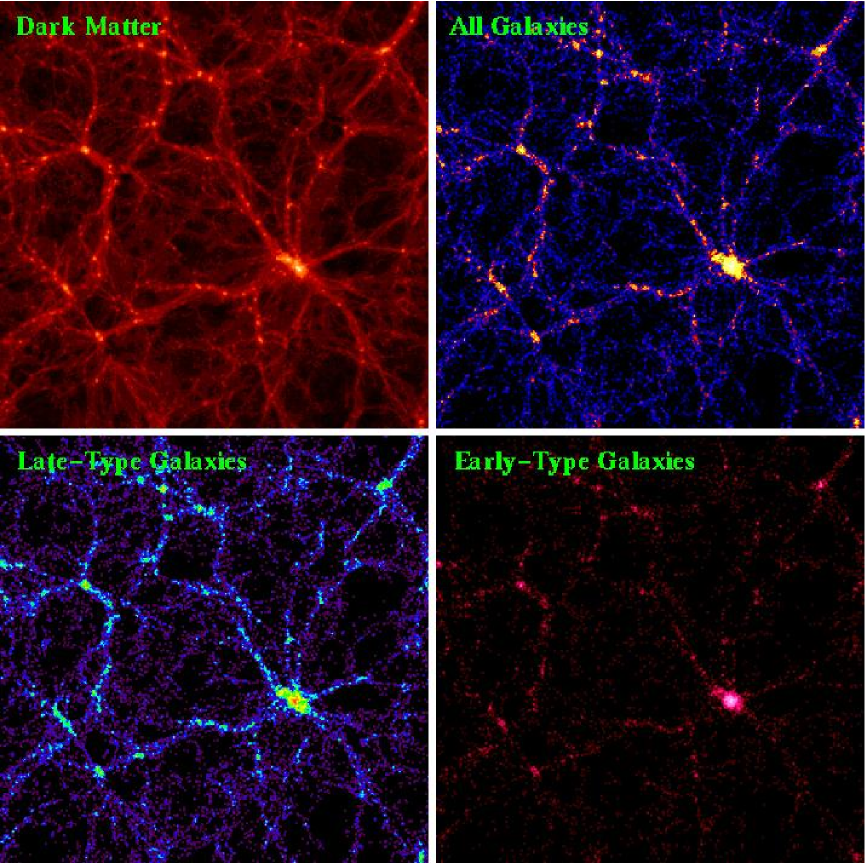
Figure 2: Projected dark matter/galaxy distributions of a $100\times 100\times 10h^{-1}\>{\rm Mpc}$ slice in one of the $L_{100}$ mock galaxy distributions. The panels show (clockwise from top-left) the dark matter particles, all galaxies (early plus late), early-type galaxies, and late-type galaxies. Galaxies are weighted by their luminosities. Note how the galaxies trace the large scale structure of the dark matter, and how early-type galaxies are more strongly clustered than late-type galaxies.

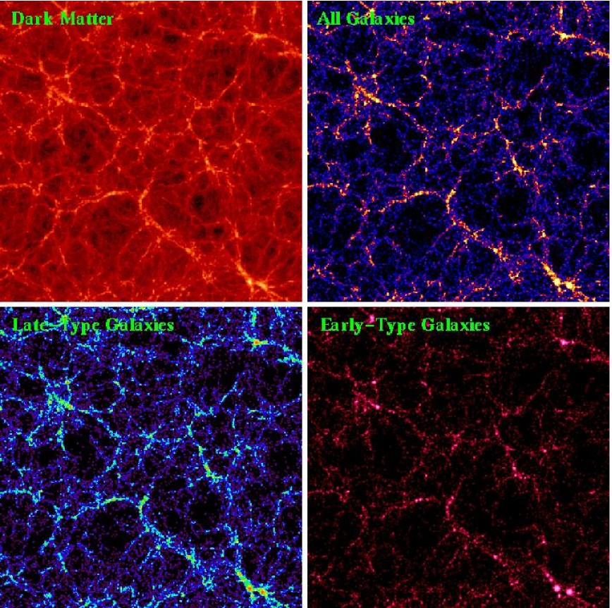
Figure 3: Same as Fig. 2, but for a $300\times 300\times 20h^{-1}\>{\rm Mpc}$ slice taken from one of the $L_{300}$ mock galaxy distributions.

3.2 Halo Occupation Numbers

When populating haloes with galaxies based on the CLF one first needs to choose a minimum luminosity. Based on the mass resolution of the simulations we adopt $L_{\rm min}=10^{7}h^{-2}\>{\rm L_{\odot}}$ throughout. The mean occupation number of galaxies with $L\geq L_{\rm min}$ for a halo with mass $M$ then follows from the CLF according to:

$$\langle N(M)\rangle=\int_{L_{\rm min}}^{\infty}\Phi(L|M)\,{\rm d}L\,.$$ (14)

In order to Monte-Carlo sample occupation numbers for individual haloes one requires the full probability distribution $P(N|M)$ (with $N$ an integer) of which $\langle N(M)\rangle$ gives the mean, i.e.,

$$\langle N(M)\rangle=\sum_{N=0}^{\infty}N\,P(N|M)$$ (15)

As a simple model we adopt

$$P(N|M)=\left\{\begin{array}[]{lll}N^{\prime}+1-\langle N(M)\rangle&\mbox{if $N=N^{\prime}$}\\ \langle N(M)\rangle-N^{\prime}&\mbox{if $N=N^{\prime}+1$}\\ 0&\mbox{otherwise}\end{array}\right.$$ (16)

Here $N^{\prime}$ is the largest integer smaller than $\langle N(M)\rangle$. Thus, the actual number of galaxies in a halo of mass $M$ is either $N^{\prime}$ or $N^{\prime}+1$. This particular model for the distribution of halo occupation numbers is supported by semi-analytical models and hydrodynamical simulations of structure formation (Benson et al. 2000; Berlind et al. 2003) which indicate that the halo occupation probability distribution is narrower than a Poisson distribution with the same mean. In addition, distribution (16) is successful in yielding power-law correlation functions, much more so than for example a Poisson distribution (Benson et al. 2000; Berlind & Weinberg 2002).

Figure 4: The luminosity functions of the mock galaxies constructed from the $L_{100}$ (left) and $L_{300}$ (right) halo catalogues (solid lines). For comparison, we also plot the LFs obtained by Madgwick et al. (2002) for all galaxies (circles), for late-type galaxies (triangles) and for early-type galaxies (stars). For clarity, the latter two LFs have been shifted down by one and two orders of magnitude in the $y$-direction, respectively. Except for incompleteness effects due to the sampling of the halo mass function (see text for details), the mock galaxy distributions have LFs that are in excellent agreement with the data.

Figure 5: The ratio of the luminosity function of mock galaxies, $\Phi_{\rm mock}(L)$, to that of the 2dFGRS, $\Phi_{\rm 2dFGRS}(L)$ (taken from Madgwick et al. 2002). The thin errorbars indicate the errors on $\Phi_{\rm 2dFGRS}(L)$. The thick solid (dashed) lines correspond to the LFs obtained from the $L_{100}$ ($L_{300}$) simulations. The errorbars for the mock galaxies are obtained from the 1-$\sigma$ variance of the two $L_{100}$ and the four $L_{300}$ simulations, respectively. See text for discussion.

3.3 Assigning galaxies their luminosity and type

Since the CLF only gives the average number of galaxies with luminosities in the range $L\pm{\rm d}L/2$ in a halo of mass $M$, there are many different ways in which one can assign luminosities to the $N_{i}$ galaxies of halo $i$, and yet be consistent with the CLF. The simplest approach would be to simply draw $N_{i}$ luminosities (with $L>L_{\rm min}$) randomly from $\Phi(L|M)$. Alternatively, one could use a more deterministic approach, and, for instance, always demand that the $j^{\rm th}$ brightest galaxy has a luminosity in the range $[L_{j},L_{j-1}]$. Here $L_{j}$ is defined such that a halo has on average $j$ galaxies with $L>L_{j}$, i.e.,

$$\int_{L_{j}}^{\infty}\Phi(L|M)dL=j\,.$$ (17)

We adopt an intermediate approach in most of our discussion, giving special treatment only to the one brightest galaxy per halo. The luminosity of this so-called “central” galaxy, $L_{c}$, is drawn from $\Phi(L|M)$ with the restriction $L>L_{1}$ and thus has an expectation value of

$$\langle L_{c}(M)\rangle=\int_{L_{1}}^{\infty}\Phi(L|M)\,L\,{\rm d}L=\tilde{\Phi}^{*}\,\tilde{L}^{*}\,\Gamma(\tilde{\alpha}+2,L_{1}/\tilde{L}^{*}),$$ (18)

The remaining $N_{i}-1$ galaxies are referred to as “satellite” galaxies and are assigned luminosities in the range $L_{\rm min}<L<L_{1}$, again drawn from the distribution function $\Phi(L|M)$. In Section 4.2, we test the effect of luminosity sampling by comparing the results obtained from all the three approaches.

Finally, the galaxies are assigned morphological types as follows. For each galaxy with luminosity $L$ in a halo of mass $M$ we draw a random number ${\cal R}$ in the range $[0,1]$. If ${\cal R}<f_{\rm late}(L,M)$ then the galaxy is a late-type, otherwise an early-type.

3.4 Assigning galaxies their phase-space coordinates

Once the population of galaxies has been assigned luminosities and types, they need to be assigned a position within their halo as well as a peculiar velocity. The central galaxy is assumed to be located at the “center” of the corresponding dark halo, which we associate with the position of the most bound particle, and its peculiar velocity is set equal to the mean halo velocity (cf. Yoshikawa, Jing & Börner 2003). For the satellite galaxies we follow two different approaches. In the first, we assign the $N_{i}-1$ satellites the positions and peculiar velocities of $N_{i}-1$ randomly selected dark matter particles that are part of the FOF halo under consideration. This thus corresponds to a scenario in which satellite galaxies are completely unbiased with respect to the density and velocity distribution of dark matter particles in FOF haloes. We refer to satellite galaxies populated this way as “FOF satellites”.

We also consider a more analytical model for the satellite distribution. This allows us first of all to assess whether a simple analytical description can be found to describe the population of satellite galaxies, and secondly, provides us with a simple framework to investigate the sensitivity of various clustering statistics to details regarding the density and velocity bias of satellite galaxies. We assume that the number density distribution of satellite galaxies follows a NFW density distribution (Navarro, Frenk & White 1997):

$$\rho(r)=\frac{\bar{\delta}\bar{\rho}}{(r/r_{\rm s})(1+r/r_{\rm s})^{2}},$$ (19)

where $r_{s}$ is a characteristic radius, $\bar{\rho}$ is the average density of the Universe, and $\bar{\delta}$ is a dimensionless amplitude which can be expressed in terms of the halo concentration parameter $c=r_{180}/r_{s}$ as

$$\bar{\delta}={180\over 3}\,{c^{3}\over{\rm ln}(1+c)-c/(1+c)}.$$ (20)

Here $r_{180}$ is the radius inside of which the halo has an average overdensity of $180$. Numerical simulations show that halo concentration depends on halo mass, and we use the relation given by Bullock et al. (2001), converted to the $c$ appropriate for our definition of halo mass. The radial number density distribution of satellite galaxies is assumed to follow equation (19) with a concentration $c_{g}=c$, and the angular position is assumed to be random over the $4\pi$ solid angle. Peculiar velocities are assumed to be the sum of the peculiar (mean) velocity of the host halo plus a random velocity which is assumed to be distributed isotropically and to follow a Gaussian, one-dimensional velocity distribution:

$$f(v_{j})={1\over\sqrt{2\pi}\sigma_{\rm gal}}\exp\left(-{v_{j}^{2}\over 2\sigma_{\rm gal}^{2}}\right).$$ (21)

Here $v_{j}$ is the velocity relative to that of the central galaxy along axis $j$, and $\sigma_{\rm gal}$ is the one-dimensional velocity dispersion of the galaxies, which we set equal to that of the dark matter particles, $\sigma_{\rm dm}$, in the halo under consideration. We refer to satellite galaxies populated this way as “NFW satellites”.

Figure 6: Two point correlation functions for dark matter particles (left panel) and mock galaxies (right panel). The dotted and dashed lines correspond to results from the $L_{300}$ and $L_{100}$ simulations, respectively. The solid line in the left panel corresponds to the evolved, non-linear correlation function for the dark matter obtained by Smith et al. (2003), and is shown for comparison. Due to the limited box-sizes, the $L_{300}$ ($L_{100}$) simulations slightly over (under) predict the correlation power on large scales with respect to Smith et al.’s model. The 2PCFs in the right panel are calculated for galaxies with absolute magnitudes $M_{b_{J}}-5\log h<-18.4$, which corresponds to the completeness limit of the $L_{300}$ MGDs. Note that the box size also affects the 2PCFs of the mock galaxies on large scales. Errorbars are the variance among the two ($L_{100}$) and four ($L_{300}$) independent realizations.

4 Results in Real Space

Fig. 2 and 3 show slices of mock galaxy distributions (hereafter MGDs) constructed from $L_{100}$ and $L_{300}$ simulations, respectively. Satellite galaxies are assigned positions and velocities using the NFW scheme outlined above. Results are shown for all galaxies (upper right panels), and separately for early types (lower right panels) and late types (lower left panels). For comparison, we also show the distribution of dark matter particles in the upper left panels. Note how the large scale structure in the dark matter distribution is delineated by the distribution of galaxies, and that early-type galaxies are more strongly clustered than late-type galaxies.

In this section we discuss the general, real-space properties of these MGDs. In Section 5 below we construct mock galaxy redshift surveys to investigate the impact of redshift distortions. The main goal of this section, however, is to investigate with what accuracy the combination of numerical simulations and our CLF analysis can be used to construct self-consistent mock galaxy distributions. In particular, we want to examine to what accuracy these MGDs can recover the input used to constrain the CLFs. Note that this is not a trivial question. The CLF modeling is based on the halo model, which only yields an approximate description of the dark matter distribution in the non-linear regime (see discussions in Cooray & Sheth 2002 and Huffenberger & Seljak 2003). In addition, as described in Section 3, the CLF alone does not yield sufficient information to construct MGDs, and we had to make additional assumptions regarding the distribution of galaxies within individual haloes. A further goal of this section, therefore, is to investigate how these assumptions impact on the clustering statistics.

4.1 The luminosity function

The CLFs used to construct the MGDs shown in Fig. 2 and 3 are constrained by the 2dFGRS luminosity functions for early- and late-type galaxies obtained by Madgwick et al. (2002). Therefore, as long as the halo mass function is well sampled by the simulations, the LFs of our MGDs should match those of Madgwick et al. (2002). Fig. 4 shows a comparison between the 2dFGRS LFs (symbols with errorbars) and the ones recovered from the MGDs (solid lines). To emphasize the level of agreement between the recovered LFs and the input LFs, Fig. 5 plots the ratio between the two. Over a large range of luminosities, the recovered LFs match the observational input extremely well. In the $L_{300}$ simulation, however, the LFs are under-estimated for $L\la 3\times 10^{9}\,h^{-2}\rm L_{\odot}$ ($M_{b_{J}}-5\log h\ga-18.4$). This owes to the absence of haloes with $M\la 2\times 10^{11}h^{-1}M_{\odot}$ (see Fig. 1). Note how this discrepancy sets in at higher $L$ for the late-type galaxies than for the early-types, because the latter are preferentially located in more massive haloes. For the early-types the $L_{300}$ mock is virtually complete down to $M_{b_{J}}-5\log h\simeq-17$ (see Fig. 10 of Paper II), reflecting the fact that only a very small fraction of the early-type galaxies brighter than this magnitude reside in haloes below the mass resolution limit. In the $L_{100}$ simulations, on the other hand, the LFs accurately match the data down to the faintest luminosities, but here the MGD underestimates the LFs at the bright end ($M_{b_{J}}-5\log h\la-22$). This owes to the limited boxsize, which causes the number of massive haloes (the main hosts of the brightest galaxies) to be underestimated (cf. Fig. 1). Note that even the LFs of the $L_{300}$ simulations underestimate the observed number of bright galaxies. This, reflects a small inaccuracy of our CLF to accurately match the observed bright end of the LFs (see paper II).

Figure 7: The real space correlation length, $r_{0}$, as a function of galaxy luminosity and type. Top panel shows the results for the combined sample of early- plus late-type galaxies, while the middle (bottom) panel shows results for the early (late) type galaxies only. Solid squares and stars correspond to the correlation lengths obtained from the $L_{300}$ and $L_{100}$ simulations, respectively. The errorbars correspond to the 1-$\sigma$ variance from the two (four) independent realizations for $L_{100}$ ($L_{300}$). We also indicate (open circles with errorbars) the correlation lengths obtained from the 2dFGRS by Norberg et al. (2002a). In the upper panel, we also plot the correlation lengths for dark matter particles for $L_{100}$ (solid line) and $L_{300}$ (dotted line) simulations. Although the agreement between data and MGDs is reasonable there are small but significant differences. The reason for these discrepancies is discussed in the text.

4.2 The real-space correlation function

In addition to the LFs of early- and late-type galaxies, the CLFs used here to construct our MGDs are also constrained by the luminosity and type dependence of the correlation lengths as measured from the 2dFGRS by Norberg et al. (2002a). Here we check to what degree this “input” is recovered from the MGDs.

The left panel of Fig. 6 plots the real-space two-point correlation functions (2PCFs) for dark matter particles in the $L_{100}$ (dashed line) and $L_{300}$ (dotted line) simulations. The solid line corresponds to the evolved, non-linear dark matter correlation function of Smith et al. (2003) and is shown for comparison. As one can see, on large scales ($r\ga 6h^{-1}{\rm Mpc}$) the correlation amplitude obtained from the $L_{100}$ simulations is systematically lower than both that obtained from the $L_{300}$ simulations and that obtained from the fitting formula of Smith et al. , suggesting that the box-size effect is non-negligible in the $L_{100}$ simulations. Note also that the large scale correlation amplitude given by the $L_{300}$ simulations is slightly higher than Smith et al. ’s model. It is unclear if this discrepancy is due to the inaccuracy of the fitting formula, or due to cosmic variance in the present simulations. As we will see below, this discrepancy limits the accuracy of model predictions.

The right-hand panel of Fig. 6 plots the 2PCFs for the galaxies in the $L_{100}$ (dashed line) and $L_{300}$ (dotted line) MGDs. Note how the galaxies reveal the same trend on large scales as the dark matter particles, with larger correlations in the $L_{300}$ than in the $L_{100}$ MGD.

Fig. 7 shows the correlation lengths $r_{0}$ as function of luminosity for all (upper panel), early-type (middle panel) and late-type (lower panel) galaxies. These have been obtained by fitting $\xi(r)$ with a power law relation of the form $\xi(r)=(r/r_{0})^{-\gamma}$ over the same range of scales as used by Norberg et al. (2002a). Solid squares and open stars correspond to correlation lengths obtained from the $L_{300}$ and $L_{100}$ MGDs, respectively. Note that the errobars on the predicted correlation lengths are based on the scatter among independent simulations boxes. They are significantly smaller than the errorbars on the observational data, because the model predictions are based on real-space correlation functions, while the observational results are based on projected correlation functions in redshift space. The agreement with the data (open circles) is reasonable, even though several systematic trends are apparent. In particular, the correlation lengths obtained from the $L_{300}$ simulation are slightly higher than the observations while the opposite applies to the $L_{100}$ simulation. These discrepancies are due to two effects. First of all, as shown in Fig. 6 the dark matter on large scales is more strongly clustered in the $L_{300}$ simulations than in the $L_{100}$ simulations. That this can account for most of the differences between the scale-lengths obtained from the $L_{300}$ and $L_{100}$ simulations, is illustrated by the dotted and solid horizontal lines, which indicate the correlation lengths of the dark matter particles in the $L_{300}$ and $L_{100}$ simulations, respectively. Secondly, the measured correlation lengths correspond to a non-zero, median redshift which is larger for the more luminous galaxies. In determining the best-fit parameters for the CLF this redshift effect is taken into account (see Papers I and II). However, in the construction of our MGDs, we only use the dark matter distribution at $z=0$. As discussed in Paper I, this can over-estimate the correlation length by about $10\%$. Given these sources of systematic errors, one should be careful not to over-interpret any discrepancy between the correlation lengths in the mock survey and those obtained from real redshift distributions.

Figure 8: The ratio of the 2PCF $\xi(r)$ in three MGDs compared to that of our fiducial MGD. The only difference among these various MGDs is the way that we assign luminosities and phase-space coordinates to the galaxies. Solid (dotted) lines correspond to a MGD in which we use a deterministic (random) method to assign galaxies their luminosities (see Section 3.3 for definitions). In the MGD corresponding to the dashed line we use the intermediate, fiducial method to assign luminosities, but here we use ‘FOF satellites’ rather than ‘NFW satellites’ (see Section 3.4 for definitions). Results are shown for galaxies in three different magnitude bins (as indicated) in one of the $L_{300}$ simulations. However, results for the $L_{100}$ simulations look virtually identical.

In order to investigate the sensitivity of the 2PCF in the MGDs to the way we assign luminosities and phase-space coordinates to the galaxies within the dark matter haloes, we construct MGDs using one of the $L_{300}$ simulations with different models for the luminosity assignment and spatial distribution of satellite galaxies within haloes. We have confirmed that using one of the $L_{100}$ simulations instead yields the same results. We first test the impact of the luminosity assignment. Here, instead of the fiducial model for the luminosity assignment (the intermediate approach discussed in Section 3.3), we use both the deterministic and random assignments (see Section  3.3 for definitions) to construct the MGDs. In Fig. 8 we shown the ratios between the correlation functions obtained from these MGDs and those obtained from the fiducial MGD. For bright galaxies, the deterministic model gives the lowest amplitudes on small scales ($r\la 1h^{-1}\>{\rm Mpc}$), while the random model gives the highest amplitudes. This is expected. The mean number of bright galaxies in a typical halo is not much larger than 1 and so not many close pairs of bright galaxies are expected in the deterministic model. More such pairs are expected in the random model because more than one galaxies in a typical halo can be assigned a large luminosity due to random fluctuations. The dashed lines in Fig. 8 correspond to a MGD with FOF satellites (see Section 3.4). The agreement of the 2PCFs between this MGD with ‘FOF satellites’ and our fiducial MGD indicate that the spherical NFW model is a good approximation of the average density distribution of dark matter haloes. We have also tested the impact of changing the concentration of galaxies, $c_{g}$; increasing (decreasing) $c_{g}$ with respect to the dark matter halo concentration, $c$, increases (decreases) the 2PCFs on small scales ($r\la 1h^{-1}\>{\rm Mpc}$). However, even when changing the ratio $c_{g}/c$ by a factor of two, the amplitude of this change is smaller than the differences resulting from changing the luminosity assignment.

All in all, changes in the way we assign luminosities and phase-space coordinates to the galaxies only have a mild impact on the 2PCFs, and only at small scales $\la 1h^{-1}\>{\rm Mpc}$. This is in good agreement with Berlind & Weinberg (2002) who have shown that these effects are much smaller than changes in the second moment of the halo occupation distributions. For example, assuming a Poissonian $P(N|M)$, rather than equation (16) has a much larger impact on the 2PCFs than any of the changes investigated above. As we show in Section 5 below, with the $P(N|M)$ of equation (16) we obtain correlation functions that are in better agreement with observations, providing empirical support for this particular occupation number distribution.

It is interesting to note that although small changes in the way we assign luminosities and phase-space coordinate do not have a big impact on the statistical measurements we are considering here, such changes can lead to quite different results for other statistical measures. As shown in van den Bosch et al. (2004), various statistics of satellite galaxies around bright galaxies can be used to distinguish models that make similar predictions about the clustering on large scales.

4.3 Pairwise velocities

The peculiar velocities of galaxies are determined by the action of the gravitational field, and so are directly related to the matter distribution in the Universe. Observationally, the properties of galaxy peculiar velocities are inferred from distortions in the correlation function. We defer this discussion to Section 5. Here we derive statistical quantities directly from the simulated peculiar velocities of galaxies.

We define the pairwise peculiar velocity of a galaxy pair as

$$v_{12}(r)\equiv[{\bf v}({\bf x}+{\bf r})-{\bf v}({\bf x})]\cdot\hat{\bf r},$$ (22)

with ${\bf v}({\bf x})$ the peculiar velocity of a galaxy at ${\bf x}$. The mean pairwise peculiar velocity and the pairwise peculiar velocity dispersion (PVD) are

$$\langle v_{12}(r)\rangle~{}~{}~{}~{}\mbox{and}~{}~{}~{}~{}\sigma_{12}(r)\equiv\langle[v_{12}(r)-\langle v_{12}(r)\rangle]^{2}\rangle^{1/2}\,,$$ (23)

where $\langle\cdot\cdot\cdot\rangle$ denotes an average over all pairs of separation $r$.

Figure 9: The mean pairwise velocities (upper panels) and pairwise velocity dispersions (lower panels) estimated from the three-dimensional (real-space) velocities of the mock galaxies and dark matter particles. All results correspond to the $L_{300}$ simulations only. Left-hand panels compare dark matter particles (solid circles) with galaxies either with NFW satellites (open circles) or with FOF satellites (open stars). Right-hand panels display the galaxy-type dependence for a model with NFW satellites (errorbars indicate the rms-scatter among the four independent $L_{300}$ simulations). See text for detailed discussion.

Figure 10: Distribution of pairwise velocities, $f(v_{12})$, for dark matter particles (solid curves), and for mock galaxies in the $L_{300}$ simulation. Results are shown for four separations $r$ as indicated, and for all galaxies (dot-dashed lines), early-type galaxies (dotted lines) and late-type galaxies (dashed lines). On small scales ($r<1h^{-1}\>{\rm Mpc}$) the pairwise velocity distributions are symmetric and reveal an obvious exponential form. On larger scales, however, $f(v_{12})$ reveals clear asymmetries: for $v_{12}<0$ the distribution is still close to an exponential, while for $v_{12}>0$ the distribution more resembles a normal distribution.

In order to gain insight, we compute $\langle v_{12}(r)\rangle$ and $\sigma_{12}(r)$ from the $L_{300}$ simulations for both dark matter particles and for galaxies with $M_{b_{J}}-5{\rm log}h\leq-18.4$ (which corresponds to the completeness limit of these simulations, see Fig. 4).

Results are shown in Fig. 9. The upper left panel compares the mean pairwise peculiar velocities of the dark matter particles (solid circles) with those of two realizations of the galaxies: one with ‘NFW satellites’ (open circles) and the other with ‘FOF satellites’ (stars). At sufficiently small separations, one probes the virialized regions of dark matter haloes, and one thus finds $\langle v_{12}\rangle=0$. At larger separations, one starts to probe the infall regions around the virialized haloes, yielding negative values for $\langle v_{12}(r)\rangle$. Finally, at sufficiently large separations $\langle v_{12}(r)\rangle\rightarrow 0$ due to the large scale homogeneity and isotropy of the Universe.

Both the dark matter particles and the galaxies from our MGDs indeed reveal such a behavior, with $\langle v_{12}(r)\rangle$ peaking at $\sim 3h^{-1}\>{\rm Mpc}$. However, there is a markedly strong difference between the $\langle v_{12}(r)\rangle$ of galaxies in the MGD with NFW satellites and that of the dark matter. In this particular MGD, the galaxies experience significantly smaller infall velocities than the dark matter particles. However, this difference between dark matter and galaxies is almost absent in the MGD with FOF satellites. This is due to the fact that in the NFW model, we populate satellites with isotropic velocity dispersions within a sphere of radius $r_{180}$. We are thus assuming that the entire region out to $r_{180}$ is virialized in that there is no net infall. However, simple collapse models predict that for our concordance cosmology only the region out to $r_{340}$ (i.e., the radius inside of which the average overdensity is 340) is virialized (Bryan & Norman 1998). The difference between the MGDs with NFW satellites and FOF satellites indicates that the regions between $r_{340}$ and $r_{180}$ are still infalling, resulting in non-zero $\langle v_{12}\rangle$.

In the lower-left panel, we compare the PVDs for galaxies and dark matter particles. Here the MGDs with FOF satellites and NFW satellites are fairly similar, and significantly lower than for the dark matter. This can be understood as follows. At small separations, the PVD is a pair weighted measure for the potential well in which dark matter particles (galaxies) reside. For the galaxies in our MGDs the halo occupation number per unit mass, $N/M$, decreases with the mass of dark matter haloes (see Paper II). Therefore, the massive haloes (with larger velocity dispersions) contribute relatively less to the PVDs of galaxies. Although the difference between the $\sigma_{12}(r)$ of the MGDs with FOF and NFW satellites shows that the PVDs have some dependence on the details regarding the infall regions around virialized haloes, these effects are typically small.

The upper-right and lower-right panels of Fig. 9 show how $\langle v_{12}(r)\rangle$ and $\sigma_{12}(r)$ depend on galaxy type. Results are shown for the MGD based on NFW satellites. The mean velocities for early-type galaxies are larger than those for late-type galaxies on large scales, but smaller on small scales. In addition, the PVD of early-type galaxies is higher than that of late-type galaxies on all scales. All these differences are easily understood as a reflection of the fact that early-type galaxies are preferentially located in the larger, more massive haloes which have larger velocity dispersions and larger infall velocities.

Fig. 10 shows the pairwise velocity distributions for four different separations $r$, within a logarithmic interval of $\Delta{\rm log}r=0.125$. On small scales, the distribution is well fit by an exponential for both dark matter particles and galaxies. This validates the assumption made in earlier analyses about this distribution (Davis & Peebles 1983; Mo, Jing & Börner 1993; Fisher et al. 1994; Marzke et al. 1995). It is also consistent with earlier results obtained from theoretical models and numerical simulations based on dark matter particles (Diaferio & Geller 1996; Sheth 1996; Mo, Jing & Börner 1997; Seto & Yokoyama 1998; Efstathiou et al. 1988; Magira, Jing & Suto 2000). For larger separations $f(v_{12})$ is skewed towards negative values of $v_{12}$, because galaxies tend to approach each other due to gravitational infall. Clearly, a single exponential function is no longer a good approximation to the pairwise peculiar velocity distribution at large separations. Although for $v_{12}<0$ (infall) the exponential remains remarkably accurate, for $v_{12}>0$ the pairwise velocity distribution reveals a more Gaussian behavior. This may have important implications for the derivation of PVDs (especially at large separations), which typically is based on the assumption of a purely exponential $f(v_{12})$. We shall return to this issue in more detail in Section 5.2.

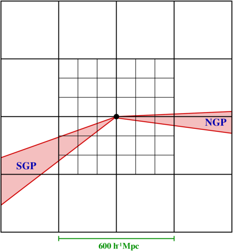
Figure 11: The stacking geometry of the $L_{100}$ and $L_{300}$ simulation boxes used to construct the MSB mock galaxy redshift surveys. The virtual observer is located at the center of the stack, indicated by a thick solid dot. Note that for MGRSs in the MB set, the stack of $6\times 6\times 6$ $L_{100}$ boxes is replaced by a stack of $2\times 2\times 2$ $L_{300}$ boxes.

5 Results in Redshift Space

The statistical quantities of galaxy clustering discussed in the previous section are based on real distances between galaxies in our MGDs. However, because of the peculiar velocities of galaxies, such quantities cannot be obtained directly from a galaxy redshift survey. On small scales the virialized motion of galaxies within dark matter haloes cause a reduction of the correlation power, while on larger scales the correlations are boosted due to the infall motion of galaxies towards overdensity regions (Kaiser 1987; Hamilton 1992). As discussed in the introduction, these distortions contain useful information about the Universal density parameter, the bias of galaxies on large (linear) scales, and the pairwise velocities of galaxies.

In this section, we use the MGDs presented above to construct large mock galaxy redshift surveys (hereafter MGRSs). The main goals are to compare various clustering statistics from these mock surveys with observational data from the 2dFGRS, and to investigate how the details about the CLF and the distribution of galaxies within haloes impact on these statistics. For the model-data comparison we use the large scale structure analysis of Hawkins et al. (2003; hereafter H03), which is based on a subsample of the 2dFGRS consisting of all galaxies located in the North Galactic Pole (NGP) and South Galactic Pole (SGP) survey strips with redshift $0.01\leq z\leq 0.20$ and apparent magnitude $b_{J}<19.3$. This sample consists of $\sim 166,000$ galaxies covering an area on the sky of $\sim 1090\,{\rm deg}^{2}$.

In order to carry out a proper comparison between model and observation, we aim to construct MGRSs that have the same selections as the 2dFGRS. First of all, the survey depth of $z_{\rm max}=0.2$ implies that we need to cover a volume with a depth of $600h^{-1}\>{\rm Mpc}$, i.e., twice that of our big $L_{300}$ simulations. In principle, we could stack $4\times 4\times 4$ identical $L_{300}$ boxes (which have periodic boundary conditions), so that a depth of $600h^{-1}\>{\rm Mpc}$ can be achieved in all directions for an observer located at the center of the stack. However, there is one problem with this set-up; as we have shown in Figs. 1 and 4 the $L_{300}$ MGD is only complete down to $M_{b_{J}}-5{\rm log}h\simeq-18.4$. Taking account of the apparent magnitude limit of the survey, this implies that our MGRSs would be incomplete out to a distance of $\sim 350h^{-1}\>{\rm Mpc}$. We can overcome this problem by using the higher resolution $L_{100}$ simulation, which is complete down to $M_{b_{J}}-5{\rm log}h\simeq-14$. We therefore replace the central $2\times 2\times 2$ $L_{300}$ boxes with a stack of $6\times 6\times 6$ $L_{100}$ boxes. The final lay-out of our virtual universe is illustrated in Figure 11. Unless stated otherwise, satellite galaxies are assigned to dark matter haloes based on our standard NFW method described in Section 3.4.

Observational selection effects, which are modelled according to the final public data release of the 2dFGRS (see also Norberg et al. 2002b), are taken into account using the following steps:

1. We place a virtual observer at the center of the stack of boxes (the solid dot in Figure 11), define a $(\alpha,\delta)$-coordinate frame, and remove all galaxies that are not located in the areas equivalent to the NGP and SGP regions of the 2dFGRS.

2. Next, for each galaxy we compute the redshift as ‘seen’ by the virtual observer. We take the observational velocity uncertainties into account by adding a random velocity drawn from a Gaussian distribution with dispersion $85\>{\rm km}\,{\rm s}^{-1}$ (Colless et al. 2001).

3. We compute the apparent magnitude of each galaxy according to its luminosity and distance. Since galaxies in the 2dFGRS were pruned by apparent magnitude before a k-correction was applied, we proceed as follows: We first apply a negative k-correction, then select galaxies according to the position-dependent magnitude limit (obtained using the apparant magnitude limit masks provided by the 2dFGRS team), and finally k-correct the magnitudes back to their rest-frame $b_{J}$-band. Throughout we use the type-dependent k-corrections given in Madgwick et al. (2002).

4. To mimic the position- and magnitude-dependent completeness of the 2dFGRS, we randomly sample each galaxy using the completeness masks provided by the 2dFGRS team. The incompleteness of the 2dFGRS parent sample is taking into account by randomly discarding $9\%$ of all mock galaxies (Norberg et al. 2002b).

5. Finally, we mimic the actual selection criteria of the 2dFGRS sample used in H03 by restricting the sample to galaxies within the redshift range $0.01\leq z\leq 0.20$ and with completeness $\geq 0.7$.

Each MGRS thus constructed contains, on average, $169000$ galaxies, with a dispersion of $\sim 5000$ due to cosmic variance. The number of galaxies in our mock catalogues are consistent with the observations at the $1\sigma$ level. Note that the correlation functions presented by H03 have been corrected for the observational bias due to fiber collisions, and we therefore do not mimic these effects in our MGRSs.

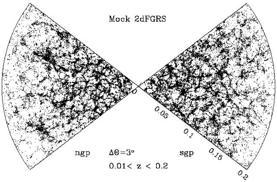
Figure 12: The distribution of a sub-set of galaxies in one of the MSB mock samples. For clarity, we plot galaxies only in two 3-degree slices, one in the ‘North Galactic Pole’ region (NGP) and the other in the ‘South Galactic Pole’ region (SGP). Only galaxies with redshifts in the range $0.01<z<0.2$ are plotted.

Since we have 2 $L_{100}$ simulations and 4 $L_{300}$ simulations, we construct $2\times 4=8$ mock catalogues with different combinations of small- and big-box simulations. In what follows, we refer to this set of mock catalogues as MSBs (for Mock Small/Big). As an example, Fig. 12 shows the distribution of a sub-set of galaxies in one of these mock catalogues. Although each of our MSB catalogs covers an extremely large volume, and should thus not be very sensitive to cosmic variance, it is constructed using simulations with box sizes of $100$ and $300h^{-1}\>{\rm Mpc}$ only. If, for instance, the $L_{100}$ simulation contains a big cluster, the $6\times 6\times 6$ reproduction of this box in our MGRSs might introduce some unrealistic features. Furthermore, as shown in Section 4.2 the $L_{100}$ box underestimates the amount of clustering on large scales. Therefore, this set of MGRSs, which replicate this box 27 times, might underestimate the clustering on large scales as well. In order to test the sensitivity of our results to these potential problems, and to have a better handle on the impact of cosmic variance in our mock surveys, we construct four alternative MGRSs. Each consists of a $4\times 4\times 4$ stack of one of the four $L_{300}$ simulations (i.e., we replace the $6\times 6\times 6$ stack of $L_{100}$ boxes by a $2\times 2\times 2$ stack of $L_{300}$ boxes). In what follows we refer to this set of mock catalogues as MBs (for Mock Big). These MGRSs, although incomplete for $M_{b_{J}}-5{\rm log}h>-18.4$, should not suffer from the lack of clustering power on large scales. The MSB set, on the other hand, does not suffer from incompleteness, but instead lacks some large scale power. As we will see below, both the MSB and MB mocks give similar results on large scales, suggesting that the box-size effect does not have a significant influence on our results.

5.1 Two-Point Correlation Functions

From our MGRSs we compute $\xi(r_{p},\pi)$ using the estimator (Hamilton 1993)

$$\xi(r_{p},\pi)={\langle RR\rangle\,\langle DD\rangle\over\langle DR\rangle^{2}}-1$$ (24)

with $\langle DD\rangle$, $\langle RR\rangle$, and $\langle DR\rangle$ the number of galaxy-galaxy, random-random, and galaxy-random pairs with separation $(r_{p},\pi)$. Here $r_{p}$ and $\pi$ are the pair separations perpendicular and parallel to the line-of-sight, respectively. Explicitly, for a pair $({\bf s_{1}},{\bf s_{2}})$, with ${\bf s_{i}}=cz_{i}{\bf\hat{r}_{i}}/H_{0}$, we define

$$\pi={{\bf s}\cdot{\bf l}\over|{\bf l}|}\;,\;\;\;\;\;\;\;\;\;\;\;\;\;\;r_{p}=\sqrt{{\bf s}\cdot{\bf s}-\pi^{2}}$$ (25)

Here ${\bf l}={1\over 2}({\bf s_{1}}+{\bf s_{2}})$ is the line of sight intersecting the pair, and ${\bf s}={\bf s_{1}}-{\bf s_{2}}$. Random samples are constructed using two different methods. The first uses the mean galaxy number density at redshift $z$ calculated from the 2dFGRS LF. The second randomizes the coordinates of all mock galaxies within the simulation box. Both methods yield indistinguishable estimates of $\xi(r_{p},\pi)$ and in what follows we only use the former. Following H03 each galaxy in a pair with redshift separation $s$ is weighted by the factor

$$w_{i}={1\over 1+4\pi n(z_{i})J_{3}(s)}$$ (26)

with $n(z)$ the number density distribution as function of redshift and $J_{3}(s)=\int_{0}^{s}\xi(s^{\prime})s^{\prime 2}{\rm d}s^{\prime}$. Hence each galaxy-galaxy, random-random, and galaxy-random pair is given a weight $w_{i}w_{j}$. We substitute $\xi(s^{\prime})$ with a power law using the same parameters as in H03. This redshift dependent weighting scheme is designed to minimize the variance on the estimated correlation function (Davis & Huchra 1982; Hamilton 1993).

Figure 13: The upper panels show the projected 2PCFs $w_{p}(r_{p})/r_{p}$ for galaxies of different luminosity and type. The errorbars correspond to the 1-$\sigma$ variance among distinct MGRSs (i.e. among the 8 MSBs for the faintest subsamples, and among the 4 MBs for the brightest subsamples). For clarity, the error bars are only plotted for the brightest and faintest subsamples. The lower panels plot the ratios of these $w_{p}(r_{p})$ to that of a reference sample. The reference sample contains all galaxies within the magnitude range $-19.5>M^{\prime}_{b_{J}}>-20.5$ (with $M^{\prime}_{b_{J}}=M_{b_{J}}-5\log h$). Note that the faintest subsamples, which are impacted by the boxsize effect of the $L_{100}$ simulation, reveal a ‘break’ at $r_{p}\simeq 10h^{-1}\>{\rm Mpc}$.

Since the redshift-space distortions only affect $\pi$, the projection of $\xi(r_{p},\pi)$ along the $\pi$ axis can get rid of these distortions and give a function that is more closely related to the real-space correlation function. In fact, this projected 2PCF is related to the real-space 2PCF through a simple Abel transform

$$w_{p}(r_{p})=\int_{-\infty}^{\infty}\xi(r_{p},\pi){\rm d}\pi=2\int_{r_{p}}^{\infty}\xi(r)\,{r\,{\rm d}r\over\sqrt{r^{2}-r_{p}^{2}}}$$ (27)

(Davis & Peebles 1983). Therefore, if the real-space 2PCF is a power-law, $\xi(r)=(r_{0}/r)^{\gamma}$, the projected 2PCF $w(r_{p})$ can be written as

$$w_{p}(r_{p})=\sqrt{\pi}\,\frac{\Gamma(\gamma/2-1/2)}{\Gamma(\gamma/2)}\,\left({r_{0}\over r_{p}}\right)^{\gamma}\,r_{p}\,.$$ (28)

We start our investigation of the redshift-space clustering properties by computing $w_{p}(r_{p})$ for a number of luminosity bins and for early- and late-type galaxies separately. To compare these projected correlation functions with the 2dFGRS results from Norberg et al. (2002a), we estimate $w_{p}(r_{p})$ using volume-limited samples with the same redshift and magnitude selection criteria as those adopted by Norberg et al. (2002a). For the MSB mocks (which use a stack of $6\times 6\times 6$ $L_{100}$ boxes), however, these $w_{p}(r_{p})$ reveal a systematic ‘break’ at $r_{p}\sim 10h^{-1}\>{\rm Mpc}$. As we have shown in Section 4.2, this owes to the fact that, because of the small box-size of the $L_{100}$ simulation, the 2PCF is too small on large scales (see Figs 6 and 7). We can circumvent this problem by using MGRSs from the the MB set, in which the stack of $6\times 6\times 6$ $L_{100}$ boxes is replaced by a stack of $2\times 2\times 2$ $L_{300}$ boxes. However, these MGRSs are only complete down to $M_{b_{J}}-5{\rm log}h\simeq-18.4$ and can therefore only be used for galaxies brighter than this.

The upper panels of Fig. 13 plot $w_{p}(r_{p})$ for different magnitude bins and for early- and late-type galaxies separately. Except for the faintest magnitude bin, these projected correlation functions are obtained from MGRS in the MB set. Results for the magnitude bin with $-17.5>M_{b_{J}}-5{\rm log}h>-18.5$ (solid lines) are obtained from the MSB set. As discussed in Paper II, the projection significantly washes out the features in the real-space 2PCFs at $\sim 2\>h^{-1}{\rm{Mpc}}$, and the projected 2PCFs better resemble a power-law. The exception is the $w_{p}(r_{p})$ for the faintest subsample of galaxies, where the ‘break’ mentioned above is clearly visible. To highlight the luminosity and type dependence of $w_{p}(r_{p})$, the lower panels of Fig. 13 plot the ratios of $w_{p}(r_{p})$ to that of a reference sample defined as all (early-type plus late-type) galaxies with $-19.5>M_{b_{J}}-5{\rm log}h>-20.5$. For a given luminosity, the correlation amplitude is higher, and the slope is steeper, for early-type galaxies than for late-type galaxies. Significant changes in the slope (and thus deviations from a perfect power-law) occur at separations $r_{p}\sim 2\>h^{-1}{\rm{Mpc}}$, which is at least qualitatively in agreement with recent results from the SDSS (Zehavi et al. 2003).

Figure 14: The correlation lengths, $r_{0}$, and slopes, $\gamma$, of the power-laws that best fit the projected correlation functions over the range $2\leq r_{p}\leq 15\>h^{-1}{\rm{Mpc}}$ (solid squares). The results for the 2 faintest luminosity bins are based on the mean and variance of the sample of 8 MSB mocks, while results for the other bins are based on the mean and variance of the sample of 4 MB mocks. Open circles with errorbars correspond to the 2dFGRS data of Norberg et al. (2002a), and are shown for comparison. Except for a systematic overestimate of the correlation lengths, the cause of which has been discussed in Section 4.2, there is good agreement between our MGRSs and the 2dFGRS.

In order to facilitate a more direct comparison with the 2dFGRS data, we fit a single power-law relation of the form (28) to these $w_{p}(r_{p})$ over the range $2\>h^{-1}{\rm{Mpc}}<r_{p}<15\>h^{-1}{\rm{Mpc}}$. This range is also adopted by Norberg et al. (2002a) when fitting the projected 2PCFs obtained from the 2dFGRS. Fig. 14 plots the real-space correlation lengths $r_{0}$ and the slopes $\gamma$ thus obtained as function of luminosity and galaxy type. The agreement between our MGRSs and the 2dFGRS is acceptable. The slight but systematic overestimate of $r_{0}$ is due to the effects discussed in Section 4.2.

We now turn to a comparison of the projected correlation function for the entire, flux limited surveys. The upper-left panel of Fig. 15 compares the $w_{p}(r_{p})$ obtained from our 8 MSB and 4 MB MGRSs with that of the 2dFGRS obtained by H03. The projected correlation functions from our MSBs and MBs agree well with each other (i.e., the 1-$\sigma$ errorbars overlap), and, at $r_{p}\ga 3h^{-1}\>{\rm Mpc}$, with the 2dFGRS results. Note that at $r_{p}\ga 10h^{-1}\>{\rm Mpc}$ the $w_{p}(r_{p})$ obtained from the MB mocks is slightly larger than that obtained from the MSB mocks, again due to the effects discussed in Section 4.2.

At large scales, $w_{p}(r_{p})$ is predominantly sensitive to the halo occupation numbers $\langle N(M)\rangle$ and virtually independent of the second moment of $P(N|M)$ or of details regarding the spatial distribution of satellite galaxies. The good agreement at large scales among different MGRSs and with the observations, therefore strongly supports our CLF and it shows that any ‘cosmic variance’ among the different MGRSs has only a relatively small impact on $w_{p}(r_{p})$. On small scales, however, the MGRSs reveal more correlation power (by about a factor 2) than observed. On such scales, $w_{p}(r_{p})$ is sensitive to our assumptions about the second moment of $P(N|M)$ and, to a lesser degree, the spatial distribution of satellite galaxies. We shall return to this small-scale mismatch and its implications in Section 6 below.

Figure 15: The projected correlation function $w_{p}(r_{p})$ (top-left panel), the redshift-space correlation function $\xi(s)$ (top-right), the quadrupole-to-monopole ratio $q(s)$ (bottom-left), and the PVDs (bottom-right) for the samples of MSB (solid lines) and MB (dashed lines) surveys. Error bars, which are similar for MB and MSB results, are only shown for the MSB results for clarity. These errorbars are based on the variance of the 8 MSB surveys. The open circles with errorbars correspond to the 2dFGRS results obtained by Hawkins et al. (2003), and are shown for comparison. Note that the MSBs and MBs give approximately the same results, but that there are marked differences between model predictions and observations. Note also that the model errorbars are in general larger than the difference in the mean between MB and MSB results, implying that these errorbars are statistical.

Rather than projecting $\xi(r_{p},\pi)$, one may also average $\xi(r_{p},\pi)$ along constant $s=\sqrt{r_{p}^{2}+\pi^{2}}$, yielding the redshift-space 2PCFs $\xi(s)$. The upper-right panel of Fig. 15 plots $\xi(s)$ obtained from our MGRSs, compared to the 2dFGRS results from H03. We find a similar behavior as with the projected correlation function; the 8 MSBs and 4 MBs agree quite well with each other and with the observations at $s\ga 6h^{-1}\>{\rm Mpc}$. At smaller redshift-space separations, however, the MGRSs slightly overpredict the correlation power. Note that the MB samples predict higher $\xi(s)$ on small scales than the MSB samples. This difference comes from the fact that the MB samples are incomplete for galaxies fainter than $M_{b_{J}}-5\log h=-18.4$. To test this we construct a mock survey from the MSB sample, but only accepting galaxies brighter than this. This yields a $\xi(s)$ in excellent agreement with that of the MB samples over all scales. Thus, although the use of only large-box simulations can results in systematic errors on small scale, the use of small-box simulations in the MSB samples does not cause any signicifant, systematic errors on large scale.

Figure 16: Same as Fig. 15 except that here we compare the results for the MSB sample with those of three alternative MGRSs in which we have modified the CLF to yield cluster mass-to-light ratios of $(M/L)_{\rm cl}=1000h\>({\rm M}/{\rm L})_{\odot}$ (dotted lines), in which we adopt a velocity bias of $b_{\rm vel}=0.6$ (dashed lines), and in which we adopt a cosmology with $\sigma_{8}=0.75$ (dot-dashed lines). All results correspond to the mean of the entire sample of 8 MSB mock surveys. For clarity, no errorbars are plotted here, but they are similar to those shown in Fig. 15. Note that both the $(M/L)_{\rm cl}=1000h\>({\rm M}/{\rm L})_{\odot}$ model and the $\sigma_{8}=0.75$ model are in good agreement with the observational data.

5.2 Redshift Space Distortions

We now turn to a comparison of the detailed shape of $\xi(r_{p},\pi)$. In particular, we focus on the distortions with respect to the real-space correlation function $\xi(r)$ induced by the peculiar velocities of galaxies.

The two-dimensional correlation function $\xi(r_{p},\pi)$ is often modeled as a convolution of the real-space 2PCF $\xi(r)$ and the conditional distribution function $f(v_{12}|r)$:

$$1+\xi(r_{p},\pi)=$$ (29)

$$\int_{-\infty}^{\infty}\left[1+\xi(\sqrt{r_{p}^{2}+(\pi-v_{12}/H_{0})^{2}})\right]\,f(v_{12}|r)\,{\rm d}v_{12}$$

(Peebles 1980). Here $v_{12}$ corresponds to the pairwise peculiar velocity along the line-of-sight and $r$ corresponds to the real-space separation. It is standard practice to assume an exponential form for $f(v_{12}|r)$ and to ignore its dependence on separation $r$ (cf., Davis & Peebles 1983; Mo, Jing & Börner 1993, 1997; Fisher et al. 1994; Marzke et al. 1995; Guzzo et al. 1997; Jing, Börner & Suto 2002; Zehavi et al. 2002). However, as we have shown in Section 4, the exponential form is only adequate at small separations, and the PVD varies quite strongly with separation. Furthermore, equation (29) is only valid for an isotropic velocity field in the limit where the probability of a real-space pair separation $r$ is independent of the probability of an associated relative velocity $v_{12}$. Although perhaps a reasonable approximation on small, highly non-linear, scales, it is certainly not valid in linear theory where the velocity and density fields are tightly coupled. In an attempt to partially correct for this, one often assumes that $f(v_{12})$ is the probability distribution for the relative velocity about the mean. Using the self-similar infall model, this mean pairwise peculiar velocity, $\langle v_{12}\rangle$, is modeled as

$$\langle v_{12}\rangle(r)=-H_{0}\,F\,\left({y\over 1+(r/r_{0})^{2}}\right)$$ (30)

(Davis & Peebles 1977) with $y=|\pi-v_{12}/H_{0}|$ the separation in real-space along the line-of-sight. $F=0$ corresponds to a Universe without any flow other than the Hubble expansion, while $F=1$ corresponds to stable clustering. Given the fairly ad hoc nature of this model, and the strong sensitivity to the uncertain value of $F$ (Davis & Peebles 1983), great care is required when interpreting any results based on this model.

A more robust model is based on linear theory and directly modeling the infall velocities around density perturbations. Following Kaiser (1987) and Hamilton (1992) one can write the observed correlation function on linear scales as

$$\xi_{\rm lin}(r_{p},\pi)=\xi_{0}(s){\cal P}_{0}(\mu)+\xi_{2}(s){\cal P}_{2}(\mu)+\xi_{4}(s){\cal P}_{4}(\mu).$$ (31)

Here ${\cal P}_{l}(\mu)$ is the $l^{th}$ Legendre polynomial, and $\mu$ is the cosine of the angle between the line-of-sight and the redshift-space separation ${\bf s}$. According to linear perturbation theory the angular moments can be written as

$$\xi_{0}(s)=\left(1+{2\beta\over 3}+{\beta^{2}\over 5}\right)\,\xi(r)\,,$$ (32)

$$\xi_{2}(s)=\left({4\beta\over 3}+{4\beta^{2}\over 7}\right)\,\left[\xi(r)-\overline{\xi}(r)\right]\,,$$ (33)

$$\xi_{4}(s)={8\beta^{2}\over 35}\,\left[\xi(r)+{5\over 2}\overline{\xi}(r)-{7\over 2}\hat{\xi}(r)\right]\,,$$ (34)

with

$$\overline{\xi}(r)={3\over r^{3}}\int_{0}^{r}\xi(r^{\prime})r^{\prime 2}{\rm d}r^{\prime}\,,$$ (35)

and

$$\hat{\xi}(r)={5\over r^{5}}\int_{0}^{r}\xi(r^{\prime})r^{\prime 4}{\rm d}r^{\prime}$$ (36)

Given a value for $\beta$ and the real-space correlation function, which can be obtained from $\xi(r_{p},\pi)$ via the projected correlation function $w_{p}(r_{p})$, equation (31) yields a model for $\xi(r_{p},\pi)$ on linear scales that takes proper account of the coupling between the density and velocity fields. To model the non-linear virialized motions of galaxies within dark matter haloes, one convolves this $\xi_{\rm lin}(r_{p},\pi)$ with the distribution function of pairwise peculiar velocities $f(v_{12}|r)$.

$$1+\xi(r_{p},\pi)=$$ (37)

$$\int_{-\infty}^{\infty}\left[1+\xi_{\rm lin}(r_{p},\pi-v_{12}/H_{0})\right]\,f(v_{12}|r)\,{\rm d}v_{12}$$

Thus, by modeling $\xi(r_{p},\pi)$ one can hope to get both an estimate of $\beta$ as well as information regarding the pairwise peculiar velocity distribution. We follow H03, and assume that the real-space 2PCF is a pure power-law, $\xi(r)=(r/r_{0})^{-\gamma}$, and that $f(v_{12}|r)$ is an exponential that is independent of the real-space separation $r$:

$$f(v_{12}|r)=f(v_{12})={1\over\sqrt{2}\sigma_{12}}{\rm exp}\left(-{\sqrt{2}|v_{12}|\over\sigma_{12}}\right)$$ (38)

Using a simple $\chi^{2}$ minimization technique, we fit these models, described by the four parameters $\beta$, $\sigma_{12}$, $r_{0}$, and $\gamma$, to the $\xi(r_{p},\pi)$ in each of our 8 MSB and 4 MB MGRSs. The $\chi^{2}$ is defined as

$$\chi^{2}=\sum\left({{\rm log}[1+\xi]_{\rm model}-{\rm log}[1+\xi]_{\rm data}\over{\rm log}[1+\xi+\Delta\xi]_{\rm data}-{\rm log}[1+\xi-\Delta\xi]_{\rm data}}\right)^{2},$$ (39)

where the summation is over the $\xi(r_{p},\pi)$ data grid with the restriction $8h^{-1}\>{\rm Mpc}<s<20h^{-1}\>{\rm Mpc}$ (see H03) and $\Delta\xi(r_{p},\pi)$ is the rms of $\xi(r_{p},\pi)$ determined from each of our 8 MSB MGRSs (or of our 4 MB MGRSs). The averages (over the 8 or the 4 MGRSs) of the best-fit values for $\beta$, $\sigma_{12}$, $r_{0}$, and $\gamma$, along with the variances among different samples, are listed in the first two lines of Table 1. These should be compared with the values listed in the last line, which correspond to the best-fit values obtained from the 2dFGRS by H03 using exactly the same method. As one can see, the best-fit values for $\beta$ and correlation lengths of the MSB and the MB sample agree with each other and with the 2dFGRS value at better than the $1\sigma$ level. On the other hand, the discrepancies regarding $\gamma$ and $\sigma_{12}$ are significant, both of which are significantly higher in our MGRSs than in the 2dFGRS.

In order to investigate these discrepancies in more detail we compute two statistics of the redshift space distortions which we compare to the 2dFGRS. As above, we take great care in using exactly the same method and assumptions as H03. Therefore, even if some aspects of the model are questionable, this allows a meaningful comparison of our results with those obtained by H03. First of all, we compute the modified quadrupole-to-monopole ratio

$$q(s)\equiv{\xi_{2}(s)\over{3\over s^{3}}\int_{0}^{s}\xi_{0}(s^{\prime})\,s^{\prime 2}\,{\rm d}s^{\prime}-\xi_{0}(s)}.$$ (40)

where $\xi_{l}(s)$ is given by

$$\xi_{l}(s)={2l+1\over 2}\int_{-1}^{1}\xi(r_{p},\pi)\,{\cal P}_{l}(\mu)\,{\rm d}\mu.$$ (41)

The lower-left panel of Fig. 15 plots $q(s)$ for MSBs and MBs together with the 2dFGRS results (open circles with errorbars). Although the MGRSs reveal the same overall behavior as the 2dFGRS data, and are mutually consistent, they systematically overpredict $q(s)$. On small scales, where random peculiar velocities cause a rapid increase of $q(s)$, this indicates that the virialized motions in our mock surveys are larger than observed (see also below). On large scales, where $q(s)$ asymptotes to the linear theory value of

$$q(s)={-{4\over 3}\beta-{4\over 7}\beta^{2}\over{1+{2\over 3}\beta+{1\over 5}\beta^{2}}}\,,$$ (42)

this might indicate that the value of $\beta$ inherent to our MGRSs is too small compared to the real Universe. On the other hand, Cole, Fisher & Weinberg (1994) have shown that non-linear, small scale power can affect $q(s)$ out to fairly large separations. Therefore the systematic overestimate of $q$ at large $s$ may simply be a reflection of the random peculiar velocities being too large, rather than an inconsistency regarding the value of $\beta$.

Table 1: Best fit parameters.

Survey	$\beta$	$r_{0}$	$\gamma$	$\sigma_{12}$
(1)	(2)	(3)	(4)	(5)
MSBs	$0.52\pm 0.05$	$5.78\pm 0.23$	$1.99\pm 0.03$	$687\pm 37$
MBs	$0.56\pm 0.06$	$5.93\pm 0.27$	$1.95\pm 0.03$	$732\pm 33$
$(M/L)_{cl}$	$0.52\pm 0.08$	$4.96\pm 0.21$	$1.88\pm 0.05$	$487\pm 44$
$b_{\rm vel}$	$0.47\pm 0.06$	$5.99\pm 0.19$	$2.00\pm 0.06$	$497\pm 47$
$\sigma_{8}$	$0.51\pm 0.06$	$5.19\pm 0.17$	$1.91\pm 0.05$	$505\pm 25$
2dFGRS	$0.49\pm 0.09$	$5.80\pm 0.25$	$1.78\pm 0.06$	$514\pm 31$

The values of $\beta$, $r_{0}$ (in $h^{-1}\>{\rm Mpc}$), $\gamma$, and $\sigma_{12}$ (in $\>{\rm km}\,{\rm s}^{-1}$) that best fit the $\xi(r_{p},\pi)$ for $8h^{-1}\>{\rm Mpc}<s<20h^{-1}\>{\rm Mpc}$ for a number of different MGRSs. Note that 4 MGRSs are used for MBs, while 8 MGRSs are used for all other cases. The quoted values are the mean and $1\sigma$ variance of these MGRSs. The MGRSs denoted by ‘$(M/L)_{\rm cl}$’ is similar to the MGRSs in the MSB set, except that here the CLF is constrained to mass-to-light ratios for clusters of $(M/L)_{\rm cl}=1000h\>({\rm M}/{\rm L})_{\odot}$, rather than $(M/L)_{\rm cl}=500h\>({\rm M}/{\rm L})_{\odot}$ as in MSB (see Section 6.3). The MGRSs denoted by ‘$b_{\rm vel}$’ is similar except for a velocity bias of $b_{\rm vel}=\sigma_{\rm gal}/\sigma_{\rm DM}=0.6$ (see Section 6.2). The MGRSs denoted by ‘$\sigma_{8}$’ is also similar except that it adopts a flat $\Lambda$CDM cosmology with $\sigma_{8}=0.75$ rather than $0.9$ (see Section 6.4). The final line lists the best-fit parameters obtained by Hawkins et al. (2003) by fitting the $\xi(r_{p},\pi)$ obtained from the 2dFGRS. Note that the errors in Hawkins et al. are estimated from the spread of 22 Mock samples.

The second statistic that we use to compare the redshift space distortions in our MGRSs with those of the 2dFGRS are the PVDs, $\sigma_{12}(r_{p})$, as a function of projected radius, $r_{p}$. Following H03, we keep $r_{0}$, $\gamma$ and $\beta$ fixed at the ‘global’ values listed in Table 1 and determine $\sigma_{12}(r_{p})$ by minimizing $\chi^{2}$ in a number of independent $r_{p}$ bins. The results are shown in the lower-right panel of Fig. 15. Whereas the 2dFGRS reveals a $\sigma_{12}(r_{p})$ that is almost constant with radius at about $500$–$600\>{\rm km}\,{\rm s}^{-1}$, our MGRSs reveal a strong increase from $\sigma_{12}\sim 600\>{\rm km}\,{\rm s}^{-1}$ at $r_{p}=0.1h^{-1}\>{\rm Mpc}$ to $\sigma_{12}\sim 900\>{\rm km}\,{\rm s}^{-1}$ at $r_{p}=1.0h^{-1}\>{\rm Mpc}$, followed by a decrease to $\sigma_{12}\sim 500\>{\rm km}\,{\rm s}^{-1}$ at $r_{p}=10h^{-1}\>{\rm Mpc}$. Thus, at around $1h^{-1}\>{\rm Mpc}$, our MGRSs dramatically overestimate the PVD. Although there is a non-negligible amount of scatter among the different mock surveys, reflecting the extreme sensitivity of the PVDs to the few richest systems in the survey, the variance among the 8 (4) MGRSs is small compared to the discrepancy.

As shown by Peacock et al. (2001) the best-fit values of $\sigma_{12}$ and $\beta$ are highly degenerate. We have tested the impact of this degeneracy on our $\sigma_{12}(r_{p})$ by repeating the same exercise using a value for $\beta$ that is $0.1$ larger (smaller) than the values listed in Table 1. This leads to an increase (decrease) of $\sigma_{12}(r_{p})$ of the order of 5 percent (20 percent) at projected radii of $1h^{-1}\>{\rm Mpc}$ ($10h^{-1}\>{\rm Mpc}$). Given that our MGRSs overpredict the PVD at $r_{p}=1h^{-1}\>{\rm Mpc}$ by about 70 percent, it is clear that this discrepancy is not a reflection of the $\beta$–$\sigma_{12}$ degeneracy. Thus, the standard $\Lambda$CDM model seems to have a severe problem in matching the observed PVDs on intermediate scales.

6 Towards a Self-Consistent Model for Large Scale Structure

Our MGRSs, based on a flat $\Lambda$CDM concordance cosmology with $\Omega_{m}=0.3$ and $\sigma_{8}=0.9$, and on a CLF that is required to yield cluster mass-to-light ratios of $(M/L)_{\rm cl}=500h\>({\rm M}/{\rm L})_{\odot}$, reveals clustering statistics that are overall in reasonable agreement with the data from the 2dFGRS. Nevertheless, two discrepancies have come to light: the MGRSs predict too much power on small scales and PVDs that are too high. We now investigate possible ways to alleviate these discrepancies.

6.1 Halo occupation models

The discrepancies between our MGRS and the 2dFGRS results might indicate a problem with our halo occupation models. Although the CLF is fairly well constrained by the observed luminosity function and the observed luminosity dependence of the correlation lengths (see Papers I and II), we have made additional assumptions regarding the second moments of the halo occupation number distributions and regarding the distribution of galaxies within individual dark matter haloes.

As we have shown in Section 4.2 the real space correlation function depends only very weakly on our method of distributing satellite galaxies within dark matter haloes (cf. Fig. 8). We have verified, using a number of tests, that modifications of the spatial distribution of satellite galaxies within dark matter haloes have no significant influence on $w_{p}(r_{p})$ or on $\sigma_{12}(r_{p})$. Therefore, none of the discrepancies mentioned above can be attributed to errors in our satellite model.

Our results are more susceptible to changes in the second moment of the halo occupation number distributions. On small scales, $\xi(r)$ scales with the average number of galaxy pairs in individual haloes $\langle{1\over 2}N(N-1)\rangle$. Therefore, one can decrease the power on small scales, to bring our $w_{p}(r_{p})$ in better agreement with observations, by lowering the second moments of our halo occupation distributions. However, our distribution (16) is already the narrowest distribution possible, and modifying the second moment of the halo occupation distributions can therefore only aggravate the discrepancies on small scales.

6.2 Velocity Bias

A seemingly obvious explanation for the too high PVDs is that the peculiar velocities of galaxies are biased with respect to the dark matter. We define the velocity bias (sometimes called ‘dynamical’ bias) as $b_{\rm vel}=\sigma_{\rm gal}/\sigma_{\rm DM}$, with $\sigma_{\rm gal}$ and $\sigma_{\rm DM}$ the peculiar velocity dispersions of (satellite) galaxies and dark matter particles in a given halo, respectively. Note that in our fiducial MGRSs we adopt $b_{\rm vel}=1$ (i.e. no velocity bias). Fig. 16 shows $w_{p}(r_{p})$, $\xi(s)$, $q(s)$ and $\sigma_{12}(r_{p})$ for MGRSs (with the MSB configuration of simulation boxes) in which $b_{\rm vel}=0.6$; i.e., the velocity dispersion of satellite galaxies is only 60 percent of that of the dark matter particles in the same halo (dashed lines). With such a pronounced velocity bias, both $q(s)$ and the PVDs, as well as $\beta$ and the global value of $\sigma_{12}$ listed in Table 1, are all consistent with the 2dFGRS results.

In two recent papers, Berlind et al. (2003) and Yoshikawa et al. (2003) measured the velocity bias of ‘galaxies’ in a smoothed particle hydrodynamics (SPH) simulation and found that $b_{\rm vel}$ decreases from $b_{\rm vel}\sim 0.9$–$1.0$ for haloes with $M\sim 3\times 10^{14}h^{-1}\>{\rm M_{\odot}}$ to $b_{\rm vel}\sim 0.6$–$0.8$ for haloes with $M\sim 3\times 10^{12}h^{-1}\>{\rm M_{\odot}}$. Thus, although simulations predict that low-mass haloes might have values for the velocity bias as low as $b_{\rm vel}\simeq 0.6$, required here to bring our PVDs in agreement with observations, the PVD is dominated by galaxies in massive haloes for which these same simulations apparently predict close to $b_{\rm vel}=1$ (i.e., no velocity bias). Furthermore, the introduction of velocity bias cannot solve the excess power on small scales. After all, the real-space correlation function is independent of $b_{\rm vel}$ such that the discrepancies regarding $w_{p}(r_{p})$ on small scales remain (see upper-left panel of Fig. 16). To make matters worse, reducing the peculiar velocities of galaxies inside dark matter haloes, increases the small scale power in redshift space. This means, that the redshift space correlation function $\xi(s)$ becomes actually more discrepant with the 2dFGRS data (see upper-right panel of Fig. 16). Therefore, although some amount of velocity bias might be expected, we do not consider it a viable solution for the problems mentioned above.

6.3 Cluster mass-to-light ratios

Because the PVD is a pair weighted statistic it is extremely sensitive to the few richest systems in the sample (i.e., Mo, Jing & Börner 1993, 1997; Zurek et al. 1994; Marzke et al. 1995; Somerville, Primack & Nolthenius 1997). The fact that the PVDs in our MGRSs are too large compared with observations therefore might indicate that either there are too many clusters of galaxies in our mock surveys (see Section 6.4 below), or that these clusters contain too many galaxies.

Our CLF was constructed under the constraint that the average mass-to-light ratio of haloes with $M\geq 10^{14}h^{-1}\>{\rm M_{\odot}}$ is equal to $(M/L)_{\rm cl}=500h\>({\rm M}/{\rm L})_{\odot}$ (in the photometric $b_{J}$ band). This value is motivated by the average mass-to-light ratio of clusters obtained by Fukugita, Hogan & Peebles (1998). To reduce the number of galaxies per cluster we now set $(M/L)_{cl}=1000h\>({\rm M}/{\rm L})_{\odot}$ and repeat the entire exercise: we first use the method described in Section 2 to compute the parameters of the new conditional luminosity function. This CLF is used to construct new MGRSs (using the same configuration of simulation boxes as in MSB), from which we determine the same statistics as before.

The results are listed in Table 1 and shown as dotted lines in Fig. 16. Clearly, increasing the mass-to-light ratio of clusters lowers $q(s)$ and $\sigma_{12}(r_{p})$, bringing them in better agreement with the 2dFGRS results. Although the PVDs are still somewhat too high, especially at around $\sim 0.4h^{-1}\>{\rm Mpc}$, the extent of this discrepancy is similar to its 1-$\sigma$ variance of the 8 MGRSs, indicating that this remaining difference is consistent with ‘cosmic variance’. As can be seen from Table 1, both $\beta$ and $\gamma$ are now in much better agreement with the 2dFGRS. In addition, the reduction of the number of galaxies in clusters significantly reduces $w_{p}(r_{p})$ at small projected separations (see Fig. 16), bringing it in good agreement with the observations . A similar reduction of small scale power is also evident in $\xi(s)$. Thus, these particular MGRSs have clustering characteristics that are overall in good agreement with the 2dFGRS results. The question is therefore whether or not such a high mass-to-light ratio for clusters of galaxies is compatible with observations.

The cluster mass-to-light ratios quoted by Fukugita et al. (1998) are $(450\pm 100)h({\rm M/L})_{\odot}$ in the $B$-band based on X-ray and velocity-dispersion data. Taking these numbers at face value, a cluster mass-to-light ratio of $(M/L)_{\rm cl}=1000h\>({\rm M}/{\rm L})_{\odot}$ is ruled out at the $5\sigma$ level. Using a variety of methods to estimate cluster masses, Bahcall et al. (2000) obtained $(M/L)_{B}=(330\pm 77)h({\rm M/L})_{\odot}$, which is consistent with the results of Carlberg et al. (1996), $(M/L)_{B}=(363\pm 65)h({\rm M/L})_{\odot}$ based on galaxy kinematics in clusters. Taking the average of these two measurements yields $\langle M/L_{B}\rangle_{\rm cl}=(350\pm 70)h\>({\rm M}/{\rm L})_{\odot}$, which rules out the cluster mass-to-light ratio required to match the clustering power on small scales at more than $7\sigma$. Thus, unless the cluster mass-to-light ratios obtained from current observations are seriously in error, increasing the average cluster mass-to-light ratio to $(M/L)_{\rm cl}\simeq 1000h\>({\rm M}/{\rm L})_{\odot}$ does not seem a viable solution for the problems at hand.

6.4 Power spectrum normalization

Rather than lowering the average number of galaxies per cluster, we may also hope to lower the PVDs by reducing the actual number of clusters. As we have shown in Section 5.2, our results, and thus the number density of rich clusters, is robust against cosmic variance. Therefore, a lower number density of clusters implies a different cosmological model. It is well known that the abundance of (rich) clusters is extremely sensitive to the power-spectrum normalization parameter $\sigma_{8}$. The too high PVDs could thus be indicative of a too high value for $\sigma_{8}$.

We therefore wish to compute the PVDs in a $\Lambda$CDM cosmology with identical cosmological parameters as before, except that $\sigma_{8}=0.75$ rather than $0.9$. Note that the choice of $\sigma_{8}=0.75$ is somewhat arbitrary, but it does represent a compromise between the constraints on the value of $\sigma_{8}$ from various observations and the low value required by our results on the PVDs (see below). In principle, constructing new MGRSs for a different cosmology requires new $N$-body simulations of the dark matter distribution. This, however, is computationally too expensive, which is why we use an approximate method instead. First, we compute the new best-fit parameters of the CLF for this cosmology, again demanding that $(M/L)_{\rm cl}=500h\>({\rm M}/{\rm L})_{\odot}$. Next we populate the dark matter haloes in our $\sigma_{8}=0.9$ simulation boxes with galaxies according to this new CLF. Finally, we construct a new sample of 8 MSB MGRSs, in which we weigh each galaxy in a halo of mass $M$ by

$$w={n(M|\sigma_{8}=0.75)\over n(M|\sigma_{8}=0.9)}$$ (43)

with $n(M)$ the number density of dark matter haloes of mass $M$. This, to first order, mimics the effect of lowering $\sigma_{8}$ on the halo mass function, and so should be a reasonable approximation on small scales where the clustering properties are determined by the galaxy distribution in individual haloes. The results for these MGRSs are shown as dot-dashed lines in Fig. 16. As one can see, the agreement with observational results in this model is much better than in the standard $\Lambda$CDM model. These results suggest that a $\Lambda$CDM model with $\sigma_{8}\sim 0.75$ may match all the observational results obtained from the 2dFGRS. Unfortunately, in the absence of proper $N$-body simulations for this model, it is impossible to make a more detailed comparison with observation.

The question is, of course, whether such a low $\sigma_{8}$ is compatible with other independent observations. Currently, the value of $\sigma_{8}$ is constrained mainly by three types of observations: weak lensing surveys, cluster mass functions, and anisotropy in the cosmic microwave background. Recent cluster abundance analyses give values of $\sigma_{8}$ (assuming $\Omega_{m}=0.3$) in a wide range, from $0.6$ to $1$ (e.g. Borgani et al. 2001; Seljak 2002; Viana, Nichol & Liddle 2002; Pen 1998; Fan & Bahcall 1998; Reiprich & Böhringer 2002). Results from weak lensing surveys are equally uncertain, with $\sigma_{8}$ spanning the range $0.7$ to $\sim 1$ (e.g., Jarvis et al. 2003; Hoekstra, Yee & Gladders 2002; Refregier et al. 2002; Bacon et al. 2003). Thus, our preferred value, $\sigma_{8}=0.75$, is consistent with these observations. At the moment, the most stringent constraint on the value of $\sigma_{8}$ is from WMAP (Spergel et al. 2003): $\sigma_{8}=0.84\pm 0.04$ ($1\sigma$ error). Even taking this result at face value, one cannot rule out $\sigma_{8}=0.75$ with any high confidence. Thus, there is no strong observational evidence to argue against a $\Lambda$CDM model with $\sigma_{8}=0.75$. Furthermore, as discussed in van den Bosch, Mo & Yang (2003), a value of $\sigma_{8}$ as low as $0.75$ can also help to alleviate several problems in current models of galaxies formation, such as the ones in connection to the Tully-Fisher relation and to the rotation curve shapes of low-surface brightness galaxies. Our results presented here give additional support for a relatively low value of $\sigma_{8}$.

7 Conclusions

In this paper, we have used realistic halo occupation distributions, obtained using the conditional luminosity function technique introduced by Yang, Mo & van den Bosch (2003), to populate dark matter haloes in high-resolution simulations of the $\Lambda$CDM ‘concordance’ cosmology. The simulations follow the evolution of $512^{3}$ dark matter particles in periodic boxes of $100h^{-1}\>{\rm Mpc}$ and $300h^{-1}\>{\rm Mpc}$ on a side. Subsequently, the dark matter haloes identified in these simulations are populated with galaxies of different luminosity and different morphological type.

We have shown that the luminosity functions and the correlation lengths as function of luminosity, both for the early- and the late-type galaxies, are in good agreement with observations. Since these same observations were used to constrain the conditional luminosity functions, which in turn were used to populate the dark matter haloes, this agreement shows that the halo occupation statistics obtained analytically can be implemented reliably in $N$-body simulations to construct realistic, self-consistent, mock galaxy distributions. We have demonstrated that the details of the spatial distribution of galaxies within individual dark matter haloes have only a very mild effect on the two-point correlation function, and only at real-space separations $r\la 0.3h^{-1}\>{\rm Mpc}$.

The mean pairwise peculiar velocities, $\langle v_{12}\rangle$, however, depend rather strongly on whether satellite galaxies (any galaxy in a dark matter halo other than the most luminous, central galaxy) are associated with random dark matter particles of the friends-of-friends (FOF) group, or whether they are assigned peculiar velocities assuming a spherical, isotropic velocity distribution around the central galaxy. In the former case, $\langle v_{12}\rangle$, which indicates the amount of infall around overdensity regions, is similar to that of the dark matter. In the latter case, $\langle v_{12}\rangle$ is significantly suppressed with respect to the dark matter. This difference indicates that the outer parts of the FOF-groups are not yet virialized.

The pairwise velocity dispersions (PVDs) of the galaxies are found to be significantly smaller than those of dark matter particles. Since the PVD is a pair weighted measure for the potential well in which dark matter particles (galaxies) reside, this can be understood as long as the average number of galaxies per unit halo mass, $N/M$, decreases with $M$ (Jing et al. 1998). Indeed, the halo occupation numbers inferred from our conditional luminosity function indicate that $N/M\propto M^{a}$ with $a\sim-0.2$.

Stacking a number of $100h^{-1}\>{\rm Mpc}$ and $300h^{-1}\>{\rm Mpc}$ simulation boxes allows us to construct mock galaxy redshift surveys (MGRSs) that are comparable to the 2dFGRS in terms of sky coverage, depth, and magnitude limit. For each of these MGRSs we estimate the two-point correlation functions $\xi(r_{p},\pi)$. These are used to derive a number of statistics about the large scale distribution of galaxies, which we compare directly with the 2dFGRS results. In particular, we calculate the projected 2PCFs $w_{p}(r_{p})$ as function of luminosity and type. The best-fit power-law slope and correlation lengths of these projected correlation functions are found in good agreement with the 2dFGRS results obtained by Norberg et al. (2002a). In addition, we also compute $w_{p}(r_{p})$ and the redshift space correlation function $\xi(s)$ for the entire MGRSs. These are compared to the 2dFGRS results obtained by Hawkins et al. (2003).

Although the agreement with the 2dFGRS data is excellent on scales larger than $\sim 3h^{-1}\>{\rm Mpc}$, on smaller scales $w_{p}(r_{p})$ is about a factor two larger than observed. To investigate this in more detail, we analyzed the redshift-space distortions present in $\xi(r_{p},\pi)$ by computing the quadrupole-to-monopole ratios $q(s)$ and the pairwise velocity dispersions $\sigma_{12}(r_{p})$. A comparison with the results of Hawkins et al. (2003) shows that the standard $\Lambda$CDM model over-predicts the clustering power on small scales by a factor of about two, and the PVDs by about $350\>{\rm km}\,{\rm s}^{-1}$. After examining a variety of possibilities, we find that the only viable solution to these problems is to reduce the power spectrum amplitude, $\sigma_{8}$, from $0.9$ to $\sim 0.75$.

No doubt, in the coming years, new results from the 2dFGRS and the SDSS will significantly improve the data on the large scale distribution of galaxies. The analysis presented here, based on the conditional luminosity function, will hopefully prove a useful tool to further constrain both galaxy formation and cosmology. In this respect, our results regarding constraints on $\sigma_{8}$ are an important illustration of the potential power of this approach.

References

- [] Bacon D., Massey R., Refregier A., Ellis R., 2003, MNRAS, 344, 673
- [] Bahcall N.A., Cen R., Davé R., Ostriker J.P., Yu Q., 2000, ApJ, 541, 1
- [] Benson A.J., Cole S., Frenk C.S., Baugh C.M., Lacey C.G., 2000, MNRAS, 311, 793
- [] Benson A.J., Baugh C.M., Cole S., Frenk C.S., Lacey C.G., 2002, MNRAS, 316, 107
- [] Berlind A.A., Weinberg D.H., 2002, ApJ, 575 587
- [] Berlind A.A., et. al., 2003, ApJ, 593, 1
- [] Borgani S., et al., 2001, ApJ, 561, 13
- [] Bullock J.S., Kolatt T.S., Sigad Y., Somerville R.S., Klypin A.A., Primack J.R., Dekel A., 2001, MNRAS, 321, 559
- [] Bullock J.S., Wechsler, R.H., Somerville R.S., 2002, MNRAS, 329, 246
- [] Bryan G., Norman M., 1998, ApJ, 495, 80
- [] Carlberg R.G., Yee H.K.C., Ellingson E., Abraham R., Gravel P., Morris S., Pritchet C.J., 1996, ApJ, 462, 32
- [] Cole S., Fisher K.B., Weinberg D.H., 1994, MNRAS, 267, 785
- [] Cole S., Hatton S., Weinberg D.H., Frenk C.S., 1998, MNRAS, 300, 945
- [] Colless M., et al., 2001, MNRAS, 328, 1039
- [] Cooray A., Sheth R., 2002, Physics Reports, 372, 1
- [] Diaferio, A., & Geller, M.J. 1996, ApJ, 467, 19
- [] Davis M., Peebles P.J.E., 1977, ApJS, 34, 425
- [] Davis M., Huchra J., 1982, ApJ, 254, 437
- [] Davis M., Peebles P.J.E., 1983, ApJ, 267, 465
- [] Davis M., Efstathiou G., Frenk C.S., White S.D.M., 1985, ApJ, 292, 371
- [] Efstathiou G., Frenk C.S., White S.D.M., Davis M., 1988, MNRAS, 235, 715
- [] Fan X., Bahcall N.A., 1998, ApJ, 504, 1
- [] Fisher K.B., Davis M., Strauss M.A., Yahil A., Huchra J.P., 1994, MNRAS, 267, 927
- [] Fukugita M., Hogan C.J., Peebles P.J.E., 1998, ApJ, 503, 518
- [] Guzzo L., Strauss M.A., Fisher K.B., Giovanelli R., Haynes M.P., 1997, ApJ, 489, 37
- [] Hamilton A.J.S., 1992, ApJ, 385, L5
- [] Hamilton A.J.S., 1993, ApJ, 417, 19
- [] Hawkins E., et al., 2003, MNRAS, in press, Preprint (astro-ph/0212375) (H03)
- [] Hoekstra, H., Yee H.K.C., Gladders M.D., 2002, ApJ, 577, 595
- [] Huffenberger K.M., Seljak U., 2003, MNRAS, 340, 1199
- [] Jarvis M., Bernstein G.M., Fischer P., Smith D., Jain B., Tyson J.A., Wittman D., 2003, AJ, 125, 1014
- [] Jing Y.P., Börner G., Suto Y., 2002, ApJ, 564, 15
- [] Jing Y.P., Mo H.J., Börner G., 1998, ApJ, 494, 1
- [] Jing Y.P., Suto, Y., 2002, ApJ, 574, 538
- [] Kaiser N., 1987, MNRAS, 227, 1
- [] Kang X., Jing Y.P., Mo H.J., Börner G., 2002, MNRAS, 336, 892
- [] Kauffmann G., Nusser A., Steinmetz M., 1997, MNRAS, 286, 795
- [] Kauffmann G., Colberg J.M., Diaferio A., White S.D.M., 1999, MNRAS, 303, 188
- [] Kochanek C.S., White M., Huchra J., Macri L., Jarrett T.H., Schneider S.E., Mader J., 2003, ApJ, 585, 161
- [] Madgwick D.S., et al., 2002, MNRAS, 333, 133
- [] Magira H., Jing Y.P., & Suto Y., 2000, 528,30
- [] Marinoni C., Hudson M.J., 2002, ApJ, 569, 101
- [] Marzke R.O., Geller M.J., Da Costa L.N., Huchra J.P., 1995, AJ, 110, 477
- [] Mathis H., Lemson G., Springel V., Kauffmann G., White S.D.M., Eldar A., Dekel A., 2002, MNRAS, 333, 739
- [] Mo H.J., Jing Y.P., Börner G., 1993, MNRAS, 264, 825
- [] Mo H.J., Jing Y.P., Börner G., 1997, MNRAS, 286, 979
- [] Navarro J.F., Frenk C.S., White S.D.M., 1997, ApJ, 490, 493
- [] Norberg P., et al., 2002a, MNRAS, 332, 827
- [] Norberg P., et al., 2002b, MNRAS, 336, 907
- [] Peacock J.A., Smith R.E., 2000, MNRAS, 318, 1144
- [] Peacock J.A., et al., 2001, Nature, 410, 169
- [] Peebles P.J.E., 1980, The Large-scale Structure of the Universe (Princeton University Press, Princeton)
- [] Pen U.-L. 1998, ApJ, 498, 60
- [] Porciani C, Dekel A, Hoffman Y, 2002, MNRAS, 332, 325
- [] Reiprich T.H., Böhringer H., 2002, ApJ, 567, 716
- [] Refregier A., Rhodes J., Groth E.J., 2002, ApJ, 572, L131
- [] Regos E., Geller M.J., 1991, ApJ, 377, 14
- [] Scoccimarro R., Sheth R.K., Hui L., Jain B., 2001, ApJ, 546, 20
- [] Scranton R., 2002, MNRAS, 332, 697
- [] Seljak U., 2000, MNRAS, 318, 203
- [] Seljak U., 2002, MNRAS, 337, 769
- [] Seto N., Yokoyama J.I. 1998, ApJ, 492, 421
- [] Sheth R.K. 1996, MNRAS, 279, 1310
- [] Sheth R.K., Mo H.J., Tormen G., 2001, MNRAS, 323, 1
- [] Sheth R.K., Tormen G., 1999, MNRAS, 308, 119
- [] Smith R.E. et al., 2003, MNRAS, 341, 1311
- [] Somerville R.S., Primack J.R., Nolthenius R., 1997, ApJ, 479, 606
- [] Somerville R.S., Lemson G., Sigad Y., Dekel A., Kauffmann G., White S.D.M., 2001, MNRAS, 320, 289
- [] Spergel D.N., et al., 2003, ApJS, 148, 175
- [] van den Bosch F.C., Yang X.H. & Mo H.J. 2003a, MNRAS, 340, 771 (Paper II)
- [] van den Bosch F.C., Mo H.J. & Yang X.H. 2003b, MNRAS, 345, 923
- [] van den Bosch F.C., Norberg P., Mo H.J., Yang X.H., Jing Y.P., 2004, MNRAS, in preparation
- [] van de Weygaert R., van Kampen E., 1993, MNRAS, 263, 481
- [] Viana P.P., Nichol R., Liddle A.R., 2002, ApJ, 569, L75
- [] White M., 2001, MNRAS, 321, 1
- [] Yang X.H., Mo H.J., & van den Bosch F.C., 2003, MNRAS, 339, 1057 (Paper I)
- [] York D., et al., 2000, AJ, 120, 1579
- [] Yoshikawa K., Jing Y.P., Börner G., 2003, ApJ, 590, 654
- [] Zehavi I., et al., 2002, ApJ, 571, 172
- [] Zehavi I., et al., 2003, preprint (astro-ph/0301280)
- [] Zheng Z., Tinker J.L., Weinberg D.H., Berlind A.A., 2002, ApJ, 575, 617
- [] Zurek W., Quinn P.J., Salmon T.K., Warren M.S., 1994, ApJ, 431, 559