Hybrid stars with color superconductivity within a nonlocal chiral quark model

Abstract

The equation of state for quark matter is derived for a nonlocal, chiral quark model within the mean field approximation. Special emphasis is on the occurrence of a diquark condensate which signals a phase transition to color superconductivity and its effects on the equation of state. We present a fit formula for the Bag pressure, which is densitiy dependent in case when the quark matter is color superconducting. We calculate the quark star configurations by solving the Tolman- Oppenheimer- Volkoff equations and demonstrate the effects of diquark condensation on the stability of hybrid stars for different formfactors of the quark interaction.

I Introduction

The investigation of color superconductivity in quark matter Barrois:1977xd ; Bailin:bm which was revived by applying nonperturbative QCD motivated interactions Rapp:1997zu ; alford99 finds most of its justification in the possible importance for the physics of compact star interiors Blaschke:uj and related observable phenomena like neutron star cooling Blaschke:1999qx ; Page:2000wt ; Blaschke:2000dy , gamma-ray bursts Hong:2001gt ; Ouyed:2001bm ; Aguilera:2002dh ; Blaschke:2003yn , gravitational wave signals for compact stars mergers Oechslin:2004yj and others Rajagopal:jq . Since calculations of quark pairing predict values of the energy gap $\Delta\sim 100$ MeV and corresponding critical temperatures for the phase transition to the superconducting state are expected to follow the BCS relation $T_{c}=0.57~{}\Delta$ for spherical wave pairing, quark matter in compact stars should always be in one of the superconducting phases.

The question arises whether conditions in compact stars allow the occurence of quark matter and the formation of stable configurations of hybrid stars. In order to give an answer to this question one has to rely on models for the equation of state which necessarily introduce free parameters and therefore some arbitrariness in the results Alford:2002rj . In particular, the question whether color superconductivity shall be realized in the 2-Flavor Superconductivity (2SC) or Color Flavor Locking (CFL) phase in the compact star interior has been discussed controversely Alford:2002kj ; Steiner:2002gx . We will restrict our further discussion to dynamical models of the NJL type with their parameters adjusted by fitting hadron properties in the vacuum before extrapolating to finite temperatures and densities within the Matsubara formalism.

Within those models it has been shown that strange quark matter occurs only at densities well above the deconfinement transition, for chemical potentials which are barely reached in the very center of a compact star Gocke:2001ri ; Buballa:2001gj ; Neumann:2002jm ; Shovkovy:2003ce ; Baldo:2002ju . The interesting and much investigated CFL phase could thus play only a marginal role for the physics of compact stars. The stability of the so obtained hybrid star configurations, however, appears to depend sensitively on details of the model, including the hadronic phase.

In the present paper we are investigating this dependence in a systematic way by employing a nonlocal chiral quark model which allows to vary the formfactor of the interaction kernel while describing the same set of hadronic vacuum properties. We provide a polynomial fit formula of our quark matter equation of state (EoS) which proves useful for applications to compact star phenomenology, as e.g. the cooling Grigorian:2003 and rotational evolution Poghosyan:2000mr or the merging Oechslin:2004yj of neutron stars. In order to compare the results of the present work for hybrid star configurations with observational constraints, we pick the example of the compact object RX J$185635-3754$, for which limits for both the mass and the radius have been reported Prakash:2002xx ; Zane:2003bp . A further restriction in the mass - radius plane of possible stable configurations comes from the constraint given by the surface redshift measurement of EXO 0748-676 Cottam:2002cu .

II Equation of state of hybrid star matter in $\beta$ equilibrium

II.1 Quark matter with color superconductivity

We consider the grand canonical thermodynamic potential for 2SC quark matter within a nonlocal chiral quark model Blaschke:2003yn where in the mean field approximation the mass gap $\phi_{f}$ and the diquark gap $\Delta$ appear as order parameters and a decomposition into color ($c\in\{r,b,g\}$) and flavor ($f\in\{u,d\}$) degrees of freedom can be made.

$$\Omega_{q}(\{\phi_{f}\},\Delta;\{\mu_{fc}\},T)=\sum_{c,f}\Omega^{c,f}(\phi_{f},\Delta;\mu_{fc},T)~{},$$ (1)

where $T$ is the temperature and $\mu_{fc}$ the chemical potential for the quark with flavor $f$ and color $c$.

The contribution of quarks with given color $c$ and flavor $f$ to the thermodynamic potential is

$$\Omega^{c,f}(\phi_{f},\Delta;\mu_{fc},T)+\Omega_{vac}^{c}=\frac{\phi_{f}^{2}}{24~{}G_{1}}+\frac{\Delta^{2}}{24~{}G_{2}}$$

$$-\frac{1}{\pi^{2}}\int^{\infty}_{0}dqq^{2}\{\omega\left[\epsilon_{c}(E_{f}(q)+\mu_{fc}),T\right]+$$

$$\omega\left[\epsilon_{c}(E_{f}(q)-\mu_{fc}),T\right]\}~{},$$ (2)

where $G_{1}$ and $G_{2}$ are coupling constants in the scalar meson and diquark channels, respectively. The dispersion relation for unpaired quarks with dynamical mass function $m_{f}(q)=m_{f}+g(q)\phi_{f}$ is given by

$$E_{f}(q)=\sqrt{q^{2}+m^{2}_{f}(q)}~{}.$$ (3)

In Eq. (2) we have introduced the notation

$$\omega\left[\epsilon_{c},T\right]=T\ln\left[1+\exp\left(-\frac{\epsilon_{c}}{T}\right)\right]+\frac{\epsilon_{c}}{2}~{},$$ (4)

where the first argument is given by

$$\epsilon_{c}(\xi)=\xi\sqrt{1+\Delta^{2}_{c}/\xi^{2}}~{}.$$ (5)

When we choose the green and blue colors to be paired and the red ones to remain unpaired, we have

$$\Delta_{c}=g(q)\Delta(\delta_{c,b}+\delta_{c,g}).$$ (6)

For a homogeneous system in equilibrium, the minimum of the thermodynamic potential $\Omega_{q}$ with respect to the order parameters $\{\phi_{f}\}$ and $\Delta$ corresponds to a negative pressure; therefore the constant $\Omega_{vac}=\sum_{c}\Omega_{vac}^{c}$ is chosen such that the pressure of the physical vacuum vanishes.

The nonlocality of the interaction between the quarks in both channels $q\bar{q}$ and $qq$ is implemented via the same formfactor functions $g(q)$ in the momentum space. In our calculations we use the Gaussian (G), Lorentzian (L) and cutoff (NJL) type formfactors defined as

$$g_{\rm G}(q) = \exp(-q^{2}/\Lambda_{\rm G}^{2})~{},$$ (7)

$$g_{\rm L}(q) = [1+(q/\Lambda_{\rm L})^{2}]^{-1},$$ (8)

$$g_{\rm NJL}(q) = \theta(1-q/\Lambda_{\rm NJL})~{}.$$ (9)

The parameter sets (quark mass $m$, coupling constant $G_{1}$, interaction range $\Lambda$) for the above formfactor models (see Tab. 1) are fixed by the pion mass $m_{\pi}=140$ MeV, pion decay constant $f_{\pi}=93$ MeV and the constituent quark mass $m_{0}=330$ MeV at $T=\mu=0$ Schmidt:di . The diquark coupling constant $G_{2}$ is a free parameter of the approach which we vary as $G_{2}=\eta~{}G_{1}$.

Following Ref. Huang:2002zd we introduce the quark chemical potential for the color $c$, $\mu_{qc}$ and the chemical potential of the isospin asymmetry, $\mu_{I}$, defined as

$$\mu_{qc} = (\mu_{uc}+\mu_{dc})/2$$ (10)

$$\mu_{I} = (\mu_{uc}-\mu_{dc})/2,$$ (11)

where the latter is color independent.

The diquark condensation in the 2SC phase induces a color asymmetry which is proportional to the chemical potential $\mu_{8}$. Therefore we can write

$$\mu_{qc}=\mu_{q}+\frac{\mu_{8}}{3}(\delta_{c,b}+\delta_{c,g}-2\delta_{c,r})~{},$$ (12)

where $\mu_{q}$ and $\mu_{8}$ are conjugate to the quark number density and the color charge density, respectively.

As has been shown in Frank:2003ve for the 2SC phase the relation $\phi_{u}=\phi_{d}=\phi$ holds so that the quark thermodynamic potential is Kiriyama:2001ud

$$\Omega_{q}(\phi,\Delta;\mu_{q},\mu_{I},\mu_{8},T)+\Omega_{vac}=\frac{\phi^{2}}{4G_{1}}+\frac{\Delta^{2}}{4G_{2}}$$

$$-\frac{1}{\pi^{2}}\int^{\infty}_{0}dqq^{2}\{\omega\left[\epsilon_{r}(-\mu_{q}+\frac{2}{3}\mu_{8}-\mu_{I}),T\right]+$$

$$\omega\left[\epsilon_{r}(\mu_{q}-\frac{2}{3}\mu_{8}-\mu_{I}),T\right]+\omega\left[\epsilon_{r}(-\mu_{q}+\frac{2}{3}\mu_{8}+\mu_{I}),T\right]+$$

$$\omega\left[\epsilon_{r}(\mu_{q}-\frac{2}{3}\mu_{8}+\mu_{I}),T\right]\}$$

$$-\frac{2}{\pi^{2}}\int^{\infty}_{0}dqq^{2}\{\omega\left[\epsilon_{b}(E(q)-\mu_{q}-\frac{1}{3}\mu_{8})-\mu_{I},T\right]+$$

$$\omega\left[\epsilon_{b}(E(q)+\mu_{q}+\frac{1}{3}\mu_{8})-\mu_{I},T\right]+$$

$$\omega\left[\epsilon_{b}(E(q)-\mu_{q}-\frac{1}{3}\mu_{8})+\mu_{I},T\right]+$$

$$\omega\left[\epsilon_{b}(E(q)+\mu_{q}+\frac{1}{3}\mu_{8})+\mu_{I},T\right]\}~{},$$ (13)

where the factor $2$ in the last integral comes from the degeneracy of the blue and green colors ($\epsilon_{b}=\epsilon_{g}$).

The total thermodynamic potential $\Omega$ contains besides the quark contribution $\Omega_{q}$ also that of the leptons $\Omega^{id}$

$$\Omega(\phi,\Delta;\mu_{q},\mu_{I},\mu_{8},\mu_{l},T) = \Omega_{q}(\phi,\Delta;\mu_{q},\mu_{I},\mu_{8},T)$$ (14)

$$+ \sum_{l\in\{e,\bar{\nu}_{e},\nu_{e}\}}\Omega^{id}(\mu_{l},T)~{}.$$

where latter are assumed to be a massless, ideal Fermi gas

$$\Omega^{id}(\mu,T)=-\frac{1}{12\pi^{2}}\mu^{4}-\frac{1}{6}\mu^{2}T^{2}-\frac{7}{180}\pi^{2}T^{4}~{}.$$ (15)

At the present stage, we do include only contributions of the first family of leptons in the thermodynamic potential.

The conditions for the local extremum of $\Omega_{q}$ correspond to coupled gap equations for the two order parameters $\phi$ and $\Delta$

$${\partial\Omega\over\partial\phi}\bigg{|}_{\phi=\phi_{0},\Delta=\Delta_{0}}={\partial\Omega\over\partial\Delta}\bigg{|}_{\phi=\phi_{0},\Delta=\Delta_{0}}=0~{}.$$ (16)

The global minimum of $\Omega_{q}$ represents the state of thermodynamic equilibrium from which all equations of state can be obtained by derivation.

II.2 Beta equilibrium, charge and color neutrality

The stellar matter in equilibrium has to obey the constraints of $\beta$-equilibrium ($d\longrightarrow u+e^{-}+\bar{\nu}_{e}$, $u+e^{-}\longrightarrow d+\nu_{e}$), expressed as

$$\mu_{dc}=\mu_{uc}+\mu_{e}~{},$$ (17)

color and electric charge neutrality and baryon number conservation.

We use in the following the electric charge density

$$Q=\frac{2}{3}\sum_{c}n_{uc}-\frac{1}{3}\sum_{c}n_{dc}-n_{e}~{},$$ (18)

the baryon number density

$$n_{B}=\frac{1}{3}\sum_{f,c}n_{fc}~{},$$ (19)

and the color number density

$$n_{8}=\frac{1}{3}\sum_{f}(n_{fb}+n_{fg}-2n_{fr})~{}.$$ (20)

The number densities $n_{j}$ occuring on the right hand sides of the above Eqs. (18) - (20) are defined as derivatives of the thermodynamic potential (14) with respect to corresponding chemical potentials $\mu_{j}$

$$n_{j}=-\frac{\partial\Omega}{\partial\mu_{j}}\bigg{|}_{\phi_{0},\Delta_{0};T,\{\mu_{j},j\not=i\}}~{},$$ (21)

Here the index $j$ stands for the particle species.

In order to express the Gibbs free enthalpy density $G$ in terms of those chemical potentials which are conjugate to the conserved densities and to implement the $\beta-$equilibrium condition (17) we make the following algebraic transformations

$$G = \sum_{f,c}\mu_{fc}n_{fc}+\mu_{e}n_{e}$$ (22)

$$= \frac{1}{3}\sum_{c}(3\mu_{qc}-\mu_{I})(n_{dc}+n_{uc})-\mu_{e}Q$$

$$= \mu_{B}~{}n_{B}+\mu_{Q}~{}Q+\mu_{8}~{}n_{8}~{},$$

where we have defined the chemical potential $\mu_{B}=3\mu_{q}-\mu_{I}$ conjugate to the baryon number density $n_{B}$ in the same way as $\mu_{Q}=-\mu_{e}$ is the chemical potential conjugate to $Q$ and $\mu_{8}$ to $n_{8}$. Then, the electric and color charge neutrality conditions read,

$$Q = 0~{},$$ (23)

$$n_{8} = 0~{},$$ (24)

at given $n_{B}$. The solution of the gap equations (16) can be performed under these constraints.

The solution of the color neutrality condition shows that $\mu_{8}$ is about $5\div 7$ MeV in the region of relevant densities ($\mu_{q}\simeq 300\div 500$ MeV). Since $\mu_{I}$ is independent of $\mu_{8}$ we consider $\mu_{qc}\simeq\mu_{q}$ ($\mu_{8}\simeq 0$) in our following calculations.

To demonstrate how to define a charge neutral state of quark matter in 2SC phase we plot in Fig. 1 the electric charge density $Q$ as a function of $\mu_{I}$ for different fixed values of $\mu_{B}$, when system is in the global minimum of the thermodynamic potential and $\eta=1$. As has been shown before in Ref. Neumann:2002jm for the NJL model case, the pure phases ($\Delta>0$: superconducting, $\Delta=0$: normal) in general are charged. These branches end at critical values of $\mu_{I}$ where their pressure is equal and the corresponding states are degenerate

$$P=P_{\Delta=0}(\mu_{B},\mu_{I},\mu_{e},T)=P_{\Delta>0}(\mu_{B},\mu_{I},\mu_{e},T)~{}.$$ (25)

In order to fulfill the charge neutrality condition one can construct a homogeneous mixed phase of these states using the Gibbs conditions Glendenning:1992vb .

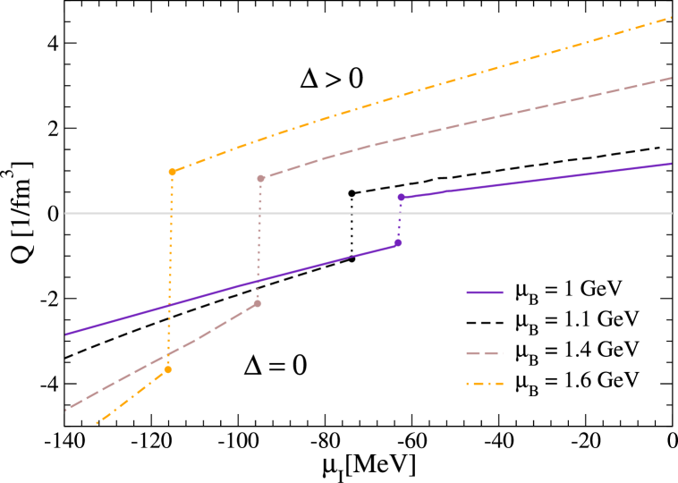
Figure 1: Electric charge density for the 2SC ($\Delta>0$) and normal ($\Delta=0$) quark matter phases as a function of $\mu_{I}$ for different fixed values of $\mu_{B}$. The end points of the lines for given $\mu_{B}$ denote states with the same pressure and represent subphases in the Glendenning construction.

The volume fraction that is occupied by the subphase with diquark condensation is defined by the charges in the subphases

$$\chi=Q_{\Delta>0}/(Q_{\Delta>0}-Q_{\Delta=0})$$ (26)

and is plotted in Fig. 2 for the different formfactor functions as a function of $\mu_{B}$.

In the same way, the number densities for the different particle species $j$ and the energy density are given by

$$n_{j}=\chi n_{j_{\Delta>0}}+(1-\chi)n_{j_{\Delta=0}}$$ (27)

$$\varepsilon=\chi\varepsilon_{\Delta>0}+(1-\chi)\varepsilon_{\Delta=0}~{}.$$ (28)

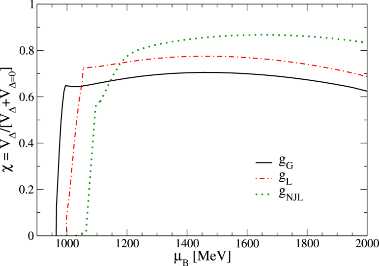
Figure 2: Volume fraction $\chi$ of the phase with nonvanishing diquark condensate obtained by a Glendenning construction of a charge-neutral mixed phase. Results are shown for three different formfactors introduced in the text.

The formulas (25)-(28) define a complete set of thermodynamic relations and can be evaluated numerically. In the next section we present the results in a form analog to the Bag model which has been widely used in the phenomenology of quark matter.

III Quark star EoS and fit formulas

We calculate the quark matter EoS within this nonlocal chiral model Blaschke:2003yn and display the results for the pressure in a form remniscent of a bag model

$$P^{(s)}=P_{id}(\mu_{B})-B^{(s)}(\mu_{B})~{},$$ (29)

where $P_{id}(\mu_{B})$ is the ideal gas pressure of quarks and $B^{(s)}(\mu_{B})$ a density dependent bag pressure, see Fig. 3. The occurrence of diquark condensation depends on the value of $\eta=G_{2}/G_{1}$ and the superscript $s\in\{S,N\}$ indicates whether we consider the matter in the superconducting mixed phase ($\eta=1$) or in the normal phase ($\eta=0$), respectively.

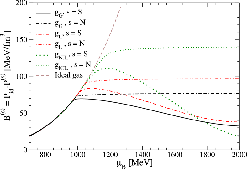
Figure 3: Bag pressure for different formfactors of the quark interaction in dependence on the baryon chemical potential for $\eta=0$ and for $\eta=1$. For the latter the superconducting phase is realized.

According to heuristic expectations, the effect of this diquark condensation (formation of quark Cooper pairs) on the EoS is similar to the occurrence of bound states and corresponds to a negative pressure contribution (Fig. 3).

For phenomenological applications of the quark matter EoS (29) we provide a polynomial fit of the bag pressure

$$B^{(s)}(\mu_{B})=\left\{\begin{array}[]{r@{~~}l}\sum_{k=0}^{10}a^{(s)}_{k}(\mu_{B}-\mu^{(s)}_{c})^{k},~{}~{}&\mu_{B}>\mu^{(s)}_{c}\\ P_{id}(\mu_{B}),~{}~{}&\mu_{B}<\mu^{(s)}_{c}\end{array}\right..$$ (32)

The coefficients $a^{(s)}_{k}$ as well as the critical chemical potential $\mu^{(s)}_{c}$ of the chiral phase transition depend on the choice of the formfactor (see Tabs. 2, 3).

The dependence of the diquark gap on the chemical potential can be represented in a similar way by the polynomial fit

$$\Delta(\mu_{B})=\left\{\begin{array}[]{r@{~~}l}\sum_{k=0}^{6}b_{k}(\mu_{B}-\mu^{(S)}_{c})^{k}~{}~{}&,~{}~{}\mu_{B}>\mu^{(S)}_{c}\\ 0~{}~{}&,~{}~{}\mu_{B}<\mu^{(S)}_{c}\end{array}\right.~{},$$ (35)

where the coefficients $b_{k}$ for the different formfactors are given in Tab. 4.

The volume fraction also can be approximated by polynomials in the following form

$$\chi(\mu_{B})=\left\{\begin{array}[]{r@{~~}l}\sum_{k=0}^{6}c_{k}(\mu_{B}-\mu^{(\chi)}_{c})^{k}~{}~{}&,~{}~{}\mu_{B}>\mu^{(\chi)}_{c}\\ \sum_{k=0}^{1}c_{k}(\mu_{B}-\mu^{(S)}_{c})^{k}~{}~{}&,~{}~{}\mu^{(\chi)}_{c}>\mu_{B}>\mu^{(S)}_{c}\\ 0~{}~{}&,~{}~{}\mu_{B}<\mu^{(S)}_{c}\end{array}\right.~{}~{}~{}.$$ (39)

The coefficients $c_{k}$ and the chemical potentials $\mu^{(\chi)}_{c}$ are given in the Table 5 for different formfactors.

IV Hadronic equation of state and phase transition

At low densities, quarks will be confined in hadrons and an appropriate EoS for dense hadron matter has to be chosen. For our discussion of quark-hadron hybrid star configurations in the next Section, we use the relativistic mean field (RMF) model of asymmmetric nuclear matter including a non-linear scalar field potential and the $\rho$ meson (nonlinear Walecka model), see Glendenning:wn . The quark-hadron phase transition is obtained using the Maxwell construction, see Refs. Voskresensky:2001jq ; Voskresensky:2002hu for a discussion. The resulting EoS is shown in Fig. 4 for the case $\eta=1$ (left panel) when the quark matter phase is superconducting and for $\eta=0$ (right panel) when it is normal.

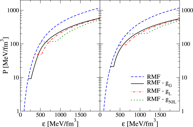
Figure 4: EoS for strongly interacting matter at zero temperature under compact stars constraints for the coupling parameter $\eta=1$ (left panel) and $\eta=0$ (right panel). Dashed line: relativistic mean-field model for hadronic matter; solid, dash-doted and doted lines correspond to quark matter with Gaussian, Lorentzian and NJL formfactor functions, respectively.

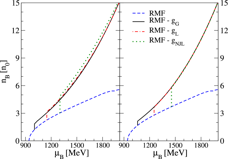
Figure 5: Baryon number density in units of the nuclear saturation density as a function of baryon chemical potential $\mu_{B}$. Left panel: $\eta=1$. Right panel: $\eta=0$. Line styles correspond to the previous figure.

When comparing the three quark model formfactors under consideration, the hardest quark matter EoS is obtained for the Gaussian, and therefore the critical pressure and corresponding critical energy densities of the deconfinement transition are the smallest, see Table 2. The same statement holds for the case $\eta=0$, when the quark matter phases are normal, see right panel of Fig. 4.

Acording to the Maxwell construction of the deconfinement phase transition, there is a jump in the energy density, as is showwn in Fig. 4.

The corresponding jumps in the baryon densities at the critical chemical potentials $\mu_{B}^{(H)}$ are given in Table 6, see also Fig. 5 for the behavoir of $n_{B}(\mu_{B})$ for all three formfactors and both cases of the diquark coupling, $\eta=1$ (left panel) and $\eta=0$ (right panel).

The EoS of hybrid stellar matter for temperature $T=0$ is relevant also for calculations of compact star cooling, since the star structure is insensitive to the temperature evolution for $T<1$ MeV.

V Configurations of hybrid stars

In this Section we consider the problem of stability of cold ($T=0$) hybrid stars with color superconducting quark matter core. The star configurations are defined from the well known Tolman-Oppenheimer-Volkoff equations Oppenheimer:1939ne , written for the hydrodynamical equilibrium of a spherically distributed matter fluid in General Relativity, see also Glendenning:wn ,

$$\frac{dP(r)}{dr}=-\frac{[\varepsilon(r)+P(r)][m(r)+4\pi r^{3}P(r)]}{r[r-2m(r)]},$$ (40)

where the mass enclosed in a sphere with distance $r$ from the center of configurations is defined by

$$m(r)=4\pi\int_{0}^{r}\varepsilon(r^{\prime})r^{\prime 2}dr^{\prime}.$$ (41)

These equations are solved for a set of central energy densities, see Figs. 6 - 9. An approximate criterion for the stability of star configurations is that masses should be rising functions of the central energy density $\varepsilon(0)$.

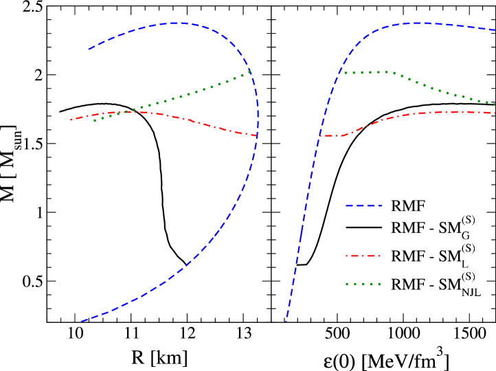
Figure 6: Mass - radius and mass - central energy density relation for compact stars configurations acording to the EoS shown in the left panel of Fig. 4. Hybrid stars with Gaussian or Lorentzian quark matter models give stable branches.

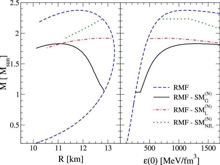
Figure 7: Same as Fig. 6 for the EoS of the right panel of Fig. 4.

Our calculations show that for the Gaussian and Lorentzian formfactors one can have stable configurations with a quark core, either with (Fig. 6) or without (Fig. 7) color superconductivity whereas for our parameterization of the NJL model (cutoff formfactor) the configurations with quark cores are not stable. For the Gaussian formfacor case the occurence of color superconductivity in quark matter shifts the critical mass of the hybrid star from $1.04$ M_⊙ to $0.62$ M_⊙ and the maximal value of the hybrid star mass from $1.83$ M_⊙ to $1.79$ M_⊙. For the Lorentzian formfactor the branch of stable hybrid stars with 2SC supercondcting quark cores lies in the mass range between $1.55$ M_⊙ and the maximum mass $1.72$ M_⊙.

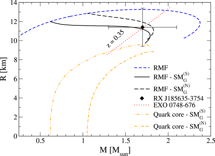
Figure 8: Radius-mass relation for Gaussian formfactor including the mass dependence of the quark core radius in both cases, one with and the other without 2SC phase.

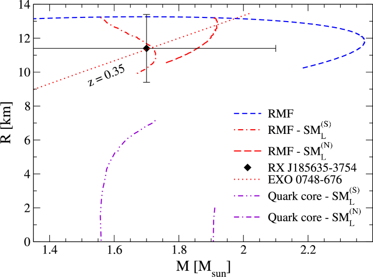
Figure 9: Same as Fig. 8 for Lorentzian formfactor.

In Figs.8 and 9 we demonstrate that these models fulfill the observational constraints from the isolated neutron star RX J$185635-3754$ Prakash:2002xx ; Zane:2003bp and from the observation of the surface redshift for EXO 0748-676 Cottam:2002cu .

The Lorentzian model with normal quark matter has marginally stable quark cores with radii less than $2$ km, in the mass range $1.91$ -$1.92~{}M_{\odot}$, see Fig. 9.

VI Conclusion

We have investigated the influence of the diquark condensation on EoS of quark matter and obtained the critical densities of phase transition to hadronic matter for different formfactors of quark interaction.

We find that the charge neutrality condition requires that the quark matter phase consists of a mixture of 2SC condensate and normal phase. The volume fraction of the condensate phase amounts to 65% - 85% depending on the formfactor function of the interaction. In the present work we did not consider muons in the quark matter phase. Their occurence would increase the volume fraction of the superconducting phase by about a 5%, helping to stabilize the 2SC phase.

We have shown that for our set of formfactors the NJL model gives no stable quark core hybrid stars. The occurence of the superconducting 2SC phase in quark matter supports the stability of the quark matter phase.

Comparison of the quark core neutron star mass-radius relation with the mass and radius of the recently observed ’small’ compact object RX J$185635-3754$ and with the constraints from the observation of the surface redshift for the object EXO 0748-676 shows that our model perfectly obeys those constraints.

These studies can be viewed as a preparatory step before more fundamental nonperturbative interactions can be provided, e.g. by QCD Schwinger-Dyson Equation studies Bender:1996bm ; Roberts:2000aa ; Maas:2002if .

Acknowlegements

We thank our colleagues for discussions and interest in our work, in particular during the NATO workshop in Yerevan, Armenia. Special thanks go to M. Buballa and D. Rischke for important remarks on a previous version of this work.

The research of D.N. Aguilera has been supported by DFG Graduiertenkolleg 567 “Stark korrelierte Vielteilchensysteme”, by CONICET PIP 03072 (Argentina), by DAAD grant No. A/01/17862 and by the Harms Stiftung of the University of Rostock. H.G. acknowledges support by DFG under grant No. 436 ARM 17/5/01 and by the Virtual Institute of the Helmholtz Association “Dense Hadronic Matter and QCD Phase Transitions” under grant No. VH-V1-041.

Form	$\Lambda$	$G_{1}~{}\Lambda^{2}$	$m$	$T_{c}(\mu=0)$	$\mu_{c}^{(S)}(T=0)$	$\mu_{c}^{(N)}(T=0)$
Factor	[GeV]		[MeV]	[MeV]	[MeV]	[MeV]
Gauss.	$1.025$	$3.7805$	$2.41$	$174$	$965$	$991$
Lor.	$0.8937$	$2.436$	$2.34$	$188$	$999$	$1045$
NJL	$0.9$	$1.944$	$5.1$	$212$	$1030$	$1100$

Table 1: Parameter sets ($\Lambda$, $G_{1}~{}\Lambda^{2}$, $m$) of the nonlocal chiral quark model for different formfactors discussed in the text. The last three columns show the critical temperatures at vanishing chemical potential and the critical chemical potentials with and without diquark condensate at vanishing temperature, respectively.

$k$	$a_{k}^{(N)}$ [GeV1-kfm-3]
	Gaussian	Lorentzian	NJL
$0$	$7.2942\cdot 10^{-2}$	$9.0218\cdot 10^{-2}$	$1.1071\cdot 10^{-1}$
$1$	$2.5122\cdot 10^{-2}$	$7.6973\cdot 10^{-2}$	$3.0219\cdot 10^{-1}$
$2$	$-9.1152\cdot 10^{-2}$	$-6.8728\cdot 10^{-1}$	$1.2820\cdot 10^{+0}$
$3$	$1.6402\cdot 10^{-1}$	$3.7260\cdot 10^{+0}$	$-4.0634\cdot 10^{+1}$
$4$	$-5.9621\cdot 10^{-3}$	$-1.1862\cdot 10^{+1}$	$3.0828\cdot 10^{+2}$
$5$	$-5.1899\cdot 10^{-1}$	$2.2342\cdot 10^{+1}$	$1.2301\cdot 10^{+3}$
$6$	$9.0892\cdot 10^{-1}$	$-2.4464\cdot 10^{+1}$	$2.9441\cdot 10^{+3}$
$7$	$-6.5617\cdot 10^{-1}$	$1.4374\cdot 10^{+1}$	$-4.3677\cdot 10^{+3}$
$8$	$1.7810\cdot 10^{-1}$	$-3.5006\cdot 10^{+0}$	$3.9376\cdot 10^{+3}$
$9$	$0$	$0$	$-1.9774\cdot 10^{+3}$
$10$	$0$	$0$	$4.2442\cdot 10^{+2}$

Table 2: Coefficients for Bag function fit formula for the normal phase case, for different formfactors Eq. (32).

$k$	$a_{k}^{(S)}$ [GeV1-kfm-3]
	Gaussian	Lorentzian	NJL
$0$	$6.5168\cdot 10^{-2}$	$7.5350\cdot 10^{-2}$	$8.4897\cdot 10^{-2}$
$1$	$1.4638\cdot 10^{-1}$	$2.8766\cdot 10^{-1}$	$2.8604\cdot 10^{-1}$
$2$	$-1.8020\cdot 10^{+0}$	$3.2215\cdot 10^{+0}$	$1.0708\cdot 10^{+0}$
$3$	$9.8125\cdot 10^{+0}$	$1.6528\cdot 10^{+1}$	$-2.8157\cdot 10^{+1}$
$4$	$-3.0515\cdot 10^{+1}$	$-4.9352\cdot 10^{+1}$	$1.6904\cdot 10^{+2}$
$5$	$5.4888\cdot 10^{+1}$	$8.7023\cdot 10^{+1}$	$-5.4828\cdot 10^{+2}$
$6$	$-5.6610\cdot 10^{+1}$	$-8.9237\cdot 10^{+1}$	$1.0896\cdot 10^{+3}$
$7$	$3.1096\cdot 10^{+1}$	$4.9210\cdot 10^{+1}$	$-1.3643\cdot 10^{+3}$
$8$	$-7.0479\cdot 10^{+0}$	$-1.1275\cdot 10^{+1}$	$1.0518\cdot 10^{+3}$
$9$	$0$	$0$	$-4.5653\cdot 10^{+2}$
$10$	$0$	$0$	$8.5443\cdot 10^{+1}$

Table 3: Coefficients for Bag function fit formula for the superconducting mixed phase, for different formfactors, Eq. (32).

$k$	$b_{k}$ [GeV1-k]
	Gaussian	Lorentzian	NJL
$0$	$9.33\cdot 10^{-2}$	$1.04\cdot 10^{-1}$	$3.30\cdot 10^{-2}$
$1$	$2.13\cdot 10^{-1}$	$1.63\cdot 10^{-1}$	$1.05\cdot 10^{0~{}}$
$2$	$-4.27\cdot 10^{-2}$	$9.19\cdot 10^{-2}$	$-3.42\cdot 10^{0~{}}$
$3$	$1.14\cdot 10^{-2}$	$-1.92\cdot 10^{-1}$	$6.13\cdot 10^{0~{}}$
$4$	$-5.27\cdot 10^{-3}$	$8.88\cdot 10^{-2}$	$-5.20\cdot 10^{0~{}}$
$5$	$0$	$0$	$1.55\cdot 10^{0~{}}$
$6$	$0$	$0$	$1.03\cdot 10^{-1}$

Table 4: Coefficients for the diquark condensate fit formula, for different formfactors, Eq. (35).

$k$	$c_{k}$ [GeV-k]
	Gaussian	Lorentzian	NJL
$\mu_{c}^{(\chi)}$[MeV]	$995$	$1054$	$1095$
	for $\mu^{(S)}_{c}<\mu_{B}<\mu^{(\chi)}_{c}$
$0$	$1.29\cdot 10^{-1}$	$8.56\cdot 10^{-2}$	$7.00\cdot 10^{-3}$
$1$	$1.66\cdot 10^{+1}$	$1.15\cdot 10^{+1}$	$8.51\cdot 10^{0~{}}$
	for $\mu^{(\chi)}_{c}<\mu_{B}$
$0$	$6.28\cdot 10^{-1}$	$7.17\cdot 10^{-1}$	$5.60\cdot 10^{-1}$
$1$	$3.36\cdot 10^{-1}$	$2.83\cdot 10^{-1}$	$2.47\cdot 10^{0~{}}$
$2$	$-3.94\cdot 10^{-1}$	$-3.43\cdot 10^{-1}$	$-7.67\cdot 10^{0~{}}$
$3$	$6.57\cdot 10^{-2}$	$-1.19\cdot 10^{-2}$	$1.06\cdot 10^{+1}$
$4$	$-8.78\cdot 10^{-3}$	$2.50\cdot 10^{-2}$	$-5.34\cdot 10^{0~{}}$
$5$	$0$	$0$	$-6.25\cdot 10^{-1}$
$6$	$0$	$0$	$7.45\cdot 10^{-1}$

Table 5: Coefficients for the volume fraction Eq. (39) and their valid ranges, for different formfactors.

	$n_{B}^{(Q)}[n_{0}]$		$n_{B}^{(H)}[n_{0}]$		$\mu_{B}^{(H)}[{\rm MeV}]$
	$\eta=1$	$\eta=0$	$\eta=1$	$\eta=0$	$\eta=1$	$\eta=0$
Gaussian	$1.84$	$2.14$	$1.20$	$1.68$	$1005$	$1059$
Lorentzian	$3.16$	$3.66$	$2.25$	$2.79$	$1149$	$1252$
NJL	$4.79$	$5.76$	$3.02$	$3.71$	$1303$	$1455$

Table 6: Limiting densities of the coexistence region between quark (Q) and hadron (H) matter phases for different formfactors ($n_{0}=0.16~{}{\rm fm}^{-3}$ is the nuclear saturation density) in the first two columns. The third column shows the critical baryon chemical potential at the phase transition $\mu_{B}^{(H)}=\mu_{B}^{(Q)}$, see Fig. 5. The subcolumns indicate the cases of superconducting ($\eta=1$) and normal ($\eta=0$) quark matter.

References

• (1) B. C. Barrois, Nucl. Phys. B 129 (1977) 390.
• (2) D. Bailin and A. Love, Phys. Rept.  107 (1984) 325.
• (3) R. Rapp, T. Schafer, E. V. Shuryak and M. Velkovsky, Phys. Rev. Lett.  81 (1998) 53 [arXiv:hep-ph/9711396].
• (4) M. Alford, K. Rajagopal and F. Wilczek, Phys. Lett. B450 (1999) 325.
• (5) D. Blaschke, N. K. Glendenning and A. Sedrakian, “Physics Of Neutron Star Interiors.” Springer Lecture Notes in Physics 578 (2001).
• (6) D. Blaschke, T. Klähn and D. N. Voskresensky, Astrophys. J.  533 (2000) 406 [arXiv:astro-ph/9908334].
• (7) D. Page, M. Prakash, J. M. Lattimer and A. Steiner, Phys. Rev. Lett.  85 (2000) 2048 [arXiv:hep-ph/0005094].
• (8) D. Blaschke, H. Grigorian and D. N. Voskresensky, Astron. Astrophys.  368 (2001) 561 [arXiv:astro-ph/0009120].
• (9) D. K. Hong, S. D. H. Hsu and F. Sannino, Phys. Lett. B 516 (2001) 362 [arXiv:hep-ph/0107017].
• (10) R. Ouyed, eConf C010815 (2002) 209.
• (11) D. N. Aguilera, D. Blaschke and H. Grigorian, arXiv:astro-ph/0212237.
• (12) D. Blaschke, S. Fredriksson, H. Grigorian and A. M. Öztas, arXiv:nucl-th/0301002.
• (13) R. Oechslin, K. Uryu, G. Poghosyan and F. K. Thielemann, arXiv:astro-ph/0401083.
• (14) K. Rajagopal, “Colour Superconductivity”, Beatenberg, High-energy physics (2001) 345-384.
• (15) M. Alford and S. Reddy, Phys. Rev. D 67 (2003) 074024 [arXiv:nucl-th/0211046].
• (16) M. Alford and K. Rajagopal, JHEP 0206 (2002) 031 [arXiv:hep-ph/0204001].
• (17) A. W. Steiner, S. Reddy and M. Prakash, Phys. Rev. D 66 (2002) 094007 [arXiv:hep-ph/0205201].
• (18) C. Gocke, D. Blaschke, A. Khalatyan and H. Grigorian, arXiv:hep-ph/0104183.
• (19) M. Buballa and M. Oertel, Nucl. Phys. A 703 (2002) 770 [arXiv:hep-ph/0109095].
• (20) F. Neumann, M. Buballa and M. Oertel, Nucl. Phys. A 714 (2003) 481 [arXiv:hep-ph/0210078].
• (21) I. Shovkovy, M. Hanauske and M. Huang, Phys. Rev. D 67 (2003) 103004 [arXiv:hep-ph/0303027].
• (22) M. Baldo, M. Buballa, F. Burgio, F. Neumann, M. Oertel and H. J. Schulze, Phys. Lett. B 562 (2003) 153 [arXiv:nucl-th/0212096].
• (23) H. Grigorian, D. Blaschke and D. N. Voskresensky, “Cooling evolution of hybrid stars with two-flavor color superconductivity,” Preprint MPG-VT-UR 231/02.
• (24) G. S. Poghosyan, H. Grigorian and D. Blaschke, Astrophys. J. 551 (2001) L73 [arXiv:astro-ph/0101002].
• (25) M. Prakash, J. M. Lattimer, A. W. Steiner and D. Page, Nucl. Phys. A 715 (2003) 835 [arXiv:astro-ph/0209122].
• (26) S. Zane, R. Turolla and J. J. Drake, arXiv:astro-ph/0302197.
• (27) J. Cottam, F. Paerels and M. Mendez, Nature 420 (2002) 51 [arXiv:astro-ph/0211126].
• (28) M. Huang, P. f. Zhuang and W. q. Chao, Phys. Rev. D 67 (2003) 065015 [arXiv:hep-ph/0207008].
• (29) M. Frank, M. Buballa and M. Oertel, Phys. Lett. B 562 (2003) 221 [arXiv:hep-ph/0303109].
• (30) O. Kiriyama, S. Yasui and H. Toki, Int. J. Mod. Phys. E 10 (2001) 501 [arXiv:hep-ph/0105170].
• (31) N. K. Glendenning, Phys. Rev. D 46 (1992) 1274.
• (32) S. M. Schmidt, D. Blaschke and Y. L. Kalinovsky, Phys. Rev. C 50 (1994) 435.
• (33) J. Berges and K. Rajagopal, Nucl. Phys. B 538 (1999) 215 [arXiv:hep-ph/9804233].
• (34) N. K. Glendenning, “Compact Stars: Nuclear Physics, Particle Physics, And General Relativity,” (Springer, New York & London, 2000).
• (35) D. N. Voskresensky, M. Yasuhira and T. Tatsumi, Phys. Lett. B 541 (2002) 93 [arXiv:nucl-th/0109009].
• (36) D. N. Voskresensky, M. Yasuhira and T. Tatsumi, Nucl. Phys. A 723 (2003) 291 [arXiv:nucl-th/0208067].
• (37) J. R. Oppenheimer and G. M. Volkoff, Phys. Rev.  55 (1939) 374.
• (38) A. Bender, D. Blaschke, Y. Kalinovsky and C. D. Roberts, Phys. Rev. Lett.  77 (1996) 3724 [arXiv:nucl-th/9606006].
• (39) C. D. Roberts and S. M. Schmidt, Prog. Part. Nucl. Phys. 45 (2001) S1 [arXiv:nucl-th/0005064].
• (40) A. Maas, B. Grüter, R. Alkofer and J. Wambach, arXiv:hep-ph/0210178.