Peculiar Velocity Limits from Measurements of the Spectrum of the Sunyaev-Zel’dovich Effect in Six Clusters of Galaxies

Abstract

We have made measurements of the Sunyaev-Zel’dovich (SZ) effect in six galaxy clusters at $z>0.2$ using the Sunyaev-Zel’dovich Infrared Experiment (SuZIE II) in three frequency bands between 150 and 350 GHz. Simultaneous multi-frequency measurements have been used to distinguish between thermal and kinematic components of the SZ effect, and to significantly reduce the effects of variations in atmospheric emission which can otherwise dominate the noise. We have set limits to the peculiar velocities of each cluster with respect to the Hubble flow, and have used the cluster sample to set a 95% confidence limit of $<1410$ km s^-1 to the bulk flow of the intermediate-redshift universe in the direction of the CMB dipole. This is the first time that SZ measurements have been used to constrain bulk flows. We show that systematic uncertainties in peculiar velocity determinations from the SZ effect are likely to be dominated by submillimeter point sources and we discuss the level of this contamination.

1 Introduction

The spectral distortion to the Cosmic Microwave Background radiation (CMB) caused by the Compton scattering of CMB photons by the hot gas in the potential wells of galaxy clusters, known as the Sunyaev-Zel’dovich (SZ) effect, is now relatively straightforward to detect and has now been measured in more than 50 sources (see Carlstrom, Holder & Reese, 2002, for a review). Single-frequency observations of the SZ effect can be used to determine the Hubble constant (Myers et al., 1997; Holzapfel et al., 1997a; Pointecouteau et al., 1999; Reese et al., 2000; Pointecouteau et al., 2001; Jones et al., 2001; De Petris et al., 2002; Reese et al., 2002) and to measure the baryon fraction in clusters (Myers et al., 1997; Grego et al., 2001).

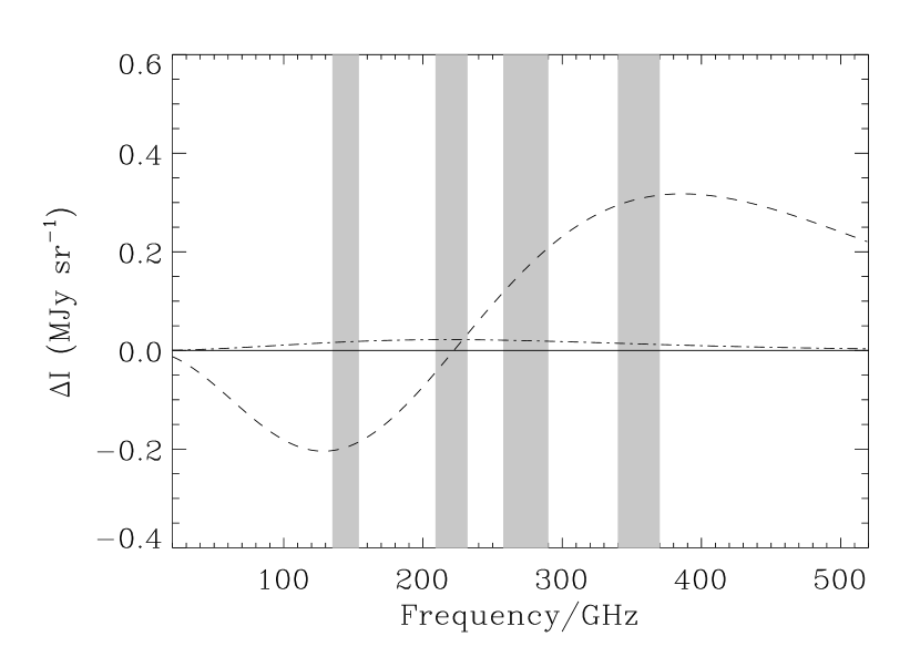
Figure 1: The frequency dependence of the SZ effect for a cluster with optical depth $\tau=0.01$, gas temperature 10 keV and a peculiar velocity of $-500$ km s^-1 (towards the observer). The thermal SZ spectrum is indicated by the dashed line; the kinematic effect by the dot-dashed line. The shaded regions indicate the bands in which SuZIE observes.

The spectrum of the SZ effect is also an important source of information. It can be approximated by the sum of two components (see Figure 1) with the strongest being the thermal SZ effect that is caused by the random thermal motions of the scattering electrons (Sunyaev & Zel’dovich, 1972). The kinematic SZ effect, due to the peculiar velocity of the intracluster (IC) gas with respect to the Hubble flow (Sunyeav & Zel’dovich, 1980), is expected to be much weaker if peculiar velocities are less than 1000 km s^-1, as favored by current models (Gramann et al., 1995; Sheth & Diaferio, 2001; Suhhonenko & Gramann, 2002). The thermal SZ effect has a distinct spectral signature, appearing as a decrement in intensity of the CMB below a frequency of $\sim$ 217 GHz, and an increment at higher frequencies (the exact frequency at which the thermal effect is zero depends on the temperature of the IC gas, as discussed by Rephaeli 1995). The kinematic effect appears as a decrement at all frequencies for a cluster that is receding with respect to the Hubble flow, and an increment at all frequencies for a cluster that is approaching. Measurements that span the null of the thermal effect are able to separate the two effects, allowing the determination of the cluster peculiar velocity (Holzapfel et al., 1997b; Mauskopf et al., 2000; LaRoque et al., 2002). Additionally, SZ spectral measurements can, in principle, be used to determine the cluster gas temperature independently of X-ray measurements (Pointecouteau, Giard & Barret, 1998; Hansen, Pastor & Semikov, 2002), the CMB temperature as a function of redshift (Rephaeli, 1980; Battistelli et al., 2002) and also to search for populations of non-thermal electrons (Shimon & Rephaeli, 2002).

Peculiar velocities probe large-scale density fluctuations and allow the distribution of matter to be determined directly without assumptions about the relationship between light and mass. Measurements of a large sample of peculiar velocities can be used to probe $\Omega_{m}$ independently of the properties of dark energy (Peel & Knox, 2002), and can, in principle, be used to reconstruct modes of the gravitational potential (Doré, Knox & Peel, 2002). The local (z$\lesssim$ 0.05) peculiar velocity field has already been measured and has been used to place tight constraints on $\Omega_{m}$ (Branchini et al., 2000; Courteau, Strauss & Willick, 2000; Courteau & Dekel, 2001; Bridle et al., 2001). However, the techniques used cannot be easily extended to higher redshifts because optical methods of distance determination have errors that increase linearly with distance. SZ spectral measurements allow peculiar velocities to be determined independently of the extragalactic distance ladder.

In this paper we describe the measurements of the SZ spectrum of 6 galaxy clusters made with the Sunyaev-Zel’dovich Infrared Experiment (SuZIE). The SuZIE II receiver makes simultaneous measurements of the SZ effect in three frequency bands, centered at 145 GHz, 221 GHz, and 355 GHz (or 270 GHz), spanning the null of the SZ thermal effect. We use these measurements to set limits on the peculiar velocity of each cluster, and to determine the cluster optical depth. The layout of this paper is as follows: in §2 we define our notation for the SZ effect; in §3 and §4 we describe the observations and data analysis. In §5 we consider statistical and systematic sources of uncertainty; in §6 we estimate the level of astrophysical confusion in our results and in §7 we determine the limits that the SuZIE peculiar velocity sample can be used to set on bulk flows, and discuss future prospects for this technique.

2 The Sunyaev-Zel’dovich Effect

2.1 The Thermal Effect

We express the CMB intensity difference caused by a distribution of high energy electrons, $n_{e}$, along the line of sight as (Rephaeli 1995):

$$\Delta I_{T}=I_{0}\frac{x^{3}}{e^{x}-1}[\Phi(x,T_{e})-1]\tau$$ (1)

where $x=h\nu/kT_{0}$, $I_{0}=2(kT_{0})^{2}/(hc)^{2}$, $T_{0}$ is the temperature of the CMB, $\tau=\int n_{e}\sigma_{T}dl$ is the optical depth of the cluster to Thomson scattering, and $\Phi(x,T_{e})$ is an integral over electron velocities and scattering directions that is specified in Rephaeli (1995). In the limit of non-relativistic electrons, this reduces to the familiar non-relativistic form for the thermal SZ effect:

$$[\Phi(x,T_{e})-1]=\frac{xe^{x}}{e^{x}-1}\left[x\frac{e^{x}+1}{e^{x}-1}-4\right]\frac{kT_{e}}{m_{e}c^{2}}$$ (2)

Following Holzapfel (1997b), we define:

$$\Psi(x,T_{e})=\frac{x^{3}}{e^{x}-1}[\Phi(x,T_{e})-1]$$ (3)

There also exist other analytic and numerical expressions for equation (1) (see Challinor & Lasenby, 1998; Itoh et al., 1998; Dolgov et al., 2001) based on a relativistic extension of the Kompaneets equation (Kompaneets, 1957). These expressions are in excellent agreement with equation (1).

We define Comptonization as $y=\tau\times(kT_{e}/m_{e}c^{2})$. It is a useful quantity because it represents a frequency independent measure of the magnitude of the SZ effect in a cluster that, unlike $\Delta I_{T}$, allows direct comparisons with other experiments.

2.2 Kinematic SZ Effect

The change in intensity of the CMB due to the non-relativistic kinematic SZ effect is:

$$\Delta I_{K}=-I_{0}\times\frac{x^{4}e^{x}}{(e^{x}-1)^{2}}\times\int n_{e}\sigma_{T}\frac{\textbf{v}_{p}}{c}\cdot\textbf{dl}$$ (4)

where $\textbf{v}_{p}$ is the bulk velocity of the IC gas relative to the CMB rest frame, and $c$ is the speed of light in units of km s ^-1. This functional form for the kinematic SZ effect has the same spectral shape as primary CMB anisotropy anisotropies, which represent a source of confusion to measurements of the kinematic effect.

An analytic expression for the relativistic kinematic SZ effect has been calculated by Nozawa et al. (1998) as a power series expansion of $\theta_{e}=kT_{e}/mc^{2}$ and $\beta=v_{p}/c$, where $v_{p}=\textbf{v}_{p}\cdot\hat{\textbf{l}}$ is the radial component to the peculiar velocity. They found the relativistic corrections to the intensity to be on the order of $+8\%$ for a cluster with electron temperature $kT_{e}=10$ keV and $v_{p}=1000$ km s^-1. Although this is a relatively small correction to our final results, we use their calculation in this paper. We express the spectral shift due to the kinematic SZ effect as:

$$\Delta I_{K}=-I_{0}\times\tau\times\frac{\textbf{v}_{p}\cdot\hat{\textbf{l}}}{c}\times h(x,T_{e})$$ (5)

where $h(x,T_{e})$ is given by:

$$h(x,T_{e})=\frac{x^{4}e^{x}}{(e^{x}-1)^{2}}\times\left[1+\theta_{e}C_{1}(x)+\theta_{e}^{2}C_{2}(x)\right]$$ (6)

and $\theta_{e}=kT_{e}/m_{e}c^{2}$. This expression includes terms up to $O(\beta\theta_{e}^{2}$). The quantities $C_{1}(x)$ and $C_{2}(x)$ are fully specified in Nozawa et al. (1998), who have also calculated corrections to equation (6) up to $O(\beta^{2})$. They find the correction from these higher order terms to be $+0.2\%$ for a cluster with $kT_{e}=10$ keV and $v_{p}=1000$ km s^-1, at a level far below the sensitivity of our observations. Therefore it can be safely ignored.

3 S-Z Observations

3.1 Instrument

In this paper we report measurements of the Sunyaev-Zeldovich effect made with the second generation Sunyaev-Zeldovich Infrared Experiment receiver (SuZIE II) at the Caltech Submillimeter Observatory (CSO) located on Mauna Kea. The SuZIE II receiver, described in Mauskopf et al. (2000) and associated references, measures the SZ effect simultaneously in three frequency bands. Two of the bands are centered at 145 and 221 GHz. The third was originally located at 273 GHz but has since been moved to 355 GHz to improve the degree to which correlated atmospheric noise can be removed from the data (Mauskopf et al., 2000). Between November 1996 and November 1997, the SuZIE II optics were changed slightly, altering both the beam size and chop throw. For a summary of the SuZIE II pass-bands and beam sizes in both configurations, see Table 1. The observations discussed in this paper include data in both configurations.

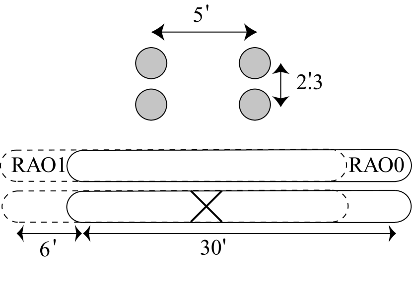
Figure 2: The upper panel shows the layout of pixels in the SuZIE II focal plane. The lower panel shows the pattern traced out on the sky by a single column of the array. The cross indicates the nominal pointing center of the observation.

The SuZIE II instrument consists of a 2 $\times$ 2 arrangement of 3-color photometers that observe the sky simultaneously in each frequency band. Each frequency is detected with a 300mK NTD Ge bolometer (Mauskopf et al., 1997). Light is coupled to the photometers through Winston horns which over-illuminate a 1.6K Lyot stop placed at the image of the primary mirror formed by a warm tertiary mirror. Each photometer defines a $\sim 1\farcm 5$ FWHM beam, with each row separated by $\sim 2\farcm 3$ and each column by $\sim 5^{\prime}$ on the sky (see Figure 2). The beam size was chosen to correspond to typical cluster sizes at intermediate redshift ($0.15\lesssim z\lesssim 0.8$). Bolometers in the same row that are sensitive to the same frequency are differenced electronically to give an effective chop throw on the sky of $5^{\prime}$. This reduces the level of common-mode atmospheric emission as well as common mode bolometer temperature, and amplifier gain, fluctuations. This differencing strategy has been discussed in detail by Holzapfel et al. (1997a) and Mauskopf et al. (2000).

3.2 Observation Strategy

Observations of six clusters were made with SuZIE II over the course of several observing runs between April 1996 and November 2000 and are summarized in Table Peculiar Velocity Limits from Measurements of the Spectrum of the Sunyaev-Zel’dovich Effect in Six Clusters of Galaxies. As shown in Figure 2, SuZIE II operates in a drift scanning mode, where the telescope is pointed ahead of the source and then parked. The earth’s rotation then causes the source to drift through the array pixels. Before each scan the dewar is rotated so that the rows of the array lie along lines of constant declination. Each scan last two minutes, or $30^{\prime}$ in right ascension, during which time the telescope maintains a fixed altitude and azimuth. After a scan is complete, the telescope reacquires the source and the scan is then repeated. Keeping the telescope fixed during an observation prevents slow drifts from changes in ground-spillover from contaminating the data. From scan to scan the initial offset of the telescope from the source (referred to in Figure 2 as RAO0 and RAO1) is alternated between $12^{\prime}$ and $18^{\prime}$, allowing a systematic check for an instrumental baseline and a check for any time dependant signals. During the observations presented here, the array was positioned so that one row passed over the center of each cluster, as specified in Table Peculiar Velocity Limits from Measurements of the Spectrum of the Sunyaev-Zel’dovich Effect in Six Clusters of Galaxies.

3.3 The Cluster Sample

We selected bright, known X-ray clusters from the ROSAT X-Ray Brightest Abell Clusters (Ebeling et al., 1996a, b) and Brightest Cluster Samples (Ebeling et al., 1998) and the Einstein Observatory Extended Medium Sensitivity Survey (Gioia et al., 1990). The observations of A1835 in April 1996 were previously analyzed by Mauskopf et al. (2000). We are using a variation of the analysis method used by Mauskopf and choose to re-analyze this data to maintain consistency between this cluster and the other data sets. We also use a slightly different X-ray model for this cluster, based on a joint analysis of radio SZ and X-ray data by Reese et al. (2002). Four of our clusters have been observed at 30 GHz by Reese et al. (2002). A comparison of our results with their measurements will be the subject of a separate paper.

3.4 Calibration

We use Mars, Uranus and Saturn for absolute calibration and to measure the beam shape of our instrument. The expected intensity of a planetary calibrator is:

$$I_{\rm plan}=\frac{\int 2k\,(\frac{\nu}{c})^{2}\,T_{\rm plan}(\nu)\,f_{k}(\nu)d\nu}{\int f_{k}({\nu})d\nu}$$ (7)

with $T_{\rm plan}(\nu)$ being the Rayleigh-Jeans (RJ) temperature of the planet, and $f_{k}(\nu)$ the transmission function of channel $k$, whose measurement is described later in this section. We correct for transmission of the atmosphere by measuring the opacity using a 225 GHz tipping tau-meter located at the CSO. This value is converted to the opacity in each of our frequency bands by calculating a scaling factor $\alpha_{k}$ which is measured from sky dips during stable atmospheric conditions. For our frequency bands at 145, 221, 273, and 355 GHz we find $\alpha=0.8,1.0,2.7,$ and $5.8$. From drift scans of the planet we measure the voltage, $V_{\rm peak}$ that is proportional to the intensity of the source. We then find our responsivity to a celestial source is:

$$R=\frac{I_{\rm plan}\Omega_{\rm plan}\times e^{-\alpha<\tau/\cos\theta_{\rm Cal}>}}{V_{peak}}\bigg{[}\frac{Jy}{V}\bigg{]}$$ (8)

where $\Omega_{\rm plan}$ is the angular size of the planet, and $<\tau/\cos\theta_{\rm Cal}>$ is averaged over the length of the observation, typically less than 20 minutes. We observe at least one calibration source every night.

The data are then calibrated by multiplying the signals by a factor of $R\times e^{\alpha<\tau/\cos\theta_{\rm SZ}>}$. We correct for the transmission of the atmosphere during each cluster observation using the same method as for the calibrator observations. Each cluster scan is multiplied by $e^{\alpha<\tau/\cos\theta_{\rm SZ}>}$, where $<\tau/\cos\theta_{\rm SZ}>$ is averaged over the length of that night’s observation of the cluster, typically less than three hours. We average the atmospheric transmission over the observation period to reduce the noise associated with the CSO tau-meter measurement system (Archibald et al., 2002). To determine whether real changes in $\tau$ over this time period could affect our results, we use the maximum variation in $<\tau/\cos\theta_{\rm SZ}>$ over a single observation, and estimate that ignoring this change contributes a $\pm$2% uncertainty in our overall calibration.

The uncertainty of $I_{\rm plan}$ is dominated by uncertainty in the measurement of $T_{\rm plan}(\nu)$. Measurements of RJ temperatures at millimeter wavelengths exist for Uranus (Griffin & Orton, 1993), Saturn and Mars (Goldin et al., 1997). Griffin & Orton model their measured Uranian temperature spectrum, $T_{\rm Uranus}(\nu)$, with a third order polynomial fit to the logarithm of wavelength. They report a 6% uncertainty in the brightness of Uranus. Goldin et al. report RJ temperatures of Mars and Saturn in four frequency bands centered between 172 and 675 GHz. From these measurements we fit a second order polynomial in frequency to model $T_{\rm Saturn}(\nu)$ and a second order polynomial in the logarithm of wavelength to model $T_{\rm Mars}(\nu)$. Goldin et al. report a $\pm$10K uncertainty to the RJ temperature of Mars due to uncertainty from their Martian atmospheric model, which translates to a 5% uncertainty in the brightness. They then use their Martian calibration to cross-calibrate their measurements of Saturn. Not including their Martian calibration error, they report a $\sim$2% uncertainty to Saturn’s RJ temperature. Adding the Martian calibration error in quadrature yields a total 5% uncertainty to the brightness of Saturn. The rings of Saturn have an effect on its millimeter wavelength emission which is hard to quantify. By cross-calibrating our Saturn measurements with SuZIE II observations of Mars and Uranus made on the same night, we have determined that ring angles between $\pm 9^{\circ}$ have a negligible effect on the total emission from Saturn. At higher ring angles we use Saturn only as a secondary calibrator. Since we use a combination of all three planets to calibrate our data, we estimate an overall $\pm$6% uncertainty to $T_{\rm planet}$.

Bolometers have a responsivity that can change with the amount of power loading on the detector; such non-linearities can potentially affect the results of calibration on a bright planet and the response of the detectors during the course of a night. We have used laboratory measurements to determine the dependence of responsivity on optical power loading. We estimate the variation in our loading from analysis of sky-dips taken at the telescope, and the calculated power received from Saturn, which is the brightest calibrator that we use. Over this range of loading conditions the maximum change in detector response is $\sim 7.0\%,8.0\%,$ and $3.5\%$ in our 145, 221, and 355 GHz frequency bands respectively. Since the responsivity change will be smaller for the majority of our observations, we assign a 6% uncertainty in the calibration error budget for this effect.

Mauskopf et al. (2000) has found that the SuZIE II beam shapes have a systematic dependence on the rotation angle of the dewar, which affects the overall calibration of the instrument. Based on these measurements we assign a $\pm$5% calibration uncertainty from this effect. Further uncertainty to the calibration arises from our measurement of the spectral response, $f_{k}(\nu)$, which affects both the intensity that we measure from the planetary calibrators and the SZ intensity. The spectral response of each SuZIE II channel was measured with a Michelson Fourier Transform Spectrometer (FTS). We then use the scatter of the measurements of the four bolometers that measure the same frequency to estimate the uncertainty in the spectral calibration at that frequency. We estimate this uncertainty to be $<$1% of the overall calibration.

The calibration uncertainties are summarized in Table 3. Adding all of these sources in quadrature, we estimate the total calibration uncertainty of SuZIE II in each of its spectral bands to be $\pm$10%.

3.5 Definition of the Data Set and Raw Data Processing

We now define some notation. Each photometer contains three bolometers each observing at a different frequency. During a scan, the six difference signals that correspond to the spatially chopped intensity on the sky at three frequencies, and in two rows, are recorded. The differenced signal is defined as:

$$D_{k}=S^{+}_{k}-S^{-}_{k}$$ (9)

where $S_{k}^{\pm}$ is the signal from each bolometer in the differenced pair. Because of the spacing of the photometers, this difference corresponds to a $5^{\prime}$ chop on the sky. The subscripts $k=1,2,3$ refer to the frequency bands of 355 GHz (or 273 GHz), 221 GHz and 145 GHz respectively in the row that is on the source. The subscripts $k=4,5,6$ refer to the same frequency set but in the row that is off-source (see Figure 2). In addition to the differenced signal, one bolometer signal from each pair is also recorded, to allow monitoring of common-mode signals. These six “single-channel” signals are referred to as $S_{k}$, where $k$ is the frequency subscript previously described. For example, the difference and single channel at 145 GHz of the on-source row will be referenced as $D_{3}$ and $S_{3}$. Both the differences and the single channels are sampled at 7 Hz.

The first step in data analysis is to remove cosmic ray spikes by carrying out a point by point differentiation of data from a single scan and looking for large ($>4\sigma$) deviations from the noise. With a knowledge of the time constant of the bolometer and the height of the spike, we can make a conservative estimate of how much data is contaminated and exclude that data from our analysis. To account for the effect of the bolometer time-constant, which is $\leq 100$ ms, we flag a region $100$ ms $\times\ln(V_{m}/\sigma)$ before, and $250$ ms $\times\ln(V_{m}/\sigma)$ after the spike’s maximum where $V_{m}$ is the height of the spike. The data are then combined into 3 second bins each containing 21 samples and covering a region equal to $0\farcm 75\cos\delta$ on the sky. Bins with 11 or more contaminated samples are excluded from further analysis. Less than 1% of the data are discarded due to cosmic ray contamination.

4 Analysis of Calibrated Data

Each cluster data set typically comprises several hundred drift scans, as summarized in Table Peculiar Velocity Limits from Measurements of the Spectrum of the Sunyaev-Zel’dovich Effect in Six Clusters of Galaxies. Once the data have been despiked, binned and calibrated, we need to extract the SZ signal from the data, and at the same time, obtain an accurate estimate of the uncertainty. For most observing conditions atmospheric emission dominates the emission from our source. Even under the best conditions the NEF for the 145 GHz channel, which is least affected by the atmosphere, is rarely below $100$ mJy s^1/2 at the signal frequencies of interest, which are $\sim 10$ mHz, while the signals we are trying to measure are $\sim 50$ mJy. The higher frequency channels are progressively worse. In order to improve our signal/noise, we make use of our ability to simultaneously measure the sum of the SZ signal and the atmosphere at three different frequencies. The different temporal and spectral behavior of the atmosphere, compared to the SZ signal of interest, allows us to clean the data and significantly improve the sensitivity of our measurements.

4.1 SZ Model

A model for the expected spatial distribution of the SZ signal in each scan is obtained by convolving a beam map of a planetary calibrator with the modelled opacity of the cluster. Beam shapes are measured by performing raster scans of a planetary calibrator and recording the voltage response of the detectors, $V_{k}(\theta,\phi)$ where $\theta$ is measured in the direction of RA and $\phi$ in the direction of declination. We approximate the electron density of the cluster with a spherically-symmetric isothermal $\beta$ model (Cavaliere & Fusco-Femiano, 1976, 1978):

$$n_{e}(r)=n_{e0}\left[1+\frac{r^{2}}{r_{c}^{2}}\right]^{-3\beta/2}$$ (10)

where $r$ is distance from the cluster center, and $\beta$ and $r_{c}$ are parameters of the model. By integrating $n_{e}$ along the line of sight, the cluster optical depth:

$$\tau(\theta,\phi)=\tau_{0}\left[1+\frac{(\theta^{2}+\phi^{2})}{\theta_{c}^{2}}\right]^{(1-3\beta)/2}$$ (11)

is obtained, where linear distance $r$ has been replaced with angles on the sky, $\theta$ and $\phi$. The model parameters of the intra-cluster gas, $\beta$ and $\theta_{c}$, for each cluster are taken from the literature and are listed in Table Peculiar Velocity Limits from Measurements of the Spectrum of the Sunyaev-Zel’dovich Effect in Six Clusters of Galaxies with associated references. We can now calculate a spatial model, $m_{k}(\theta)$, for each cluster:

$$m_{k}(\theta)=\int\int\frac{V_{k}(\theta^{\prime},\phi^{\prime})}{V_{peak}}\frac{\tau(\theta^{\prime}-\theta,\phi^{\prime})}{\tau_{0}}d\theta^{\prime}d\phi^{\prime}$$ (12)

that has units of steradians, and is calculated at $0^{\prime}.05\times cos\delta$ intervals for a given offset, $\theta$, in right ascension from the cluster center. We calculate our SZ model by multiplying the source model by thermal and kinematic band-averaged spectral factors given by:

$$T_{k}=I_{0}\times\frac{m_{e}c^{2}}{kT_{e}}\times\frac{\int\Psi(x,T_{e})\times f_{k}(x)dx}{\int f_{k}(x)dx}$$ (13)

and

$$K_{k}=-I_{0}\times\frac{m_{e}c^{2}}{kT_{e}}\times\frac{\mathbf{\hat{n}}_{v}\cdot\mathbf{\hat{l}}}{c}\times\frac{\int h(x,T_{e})\times f_{k}(x)dx}{\int f_{k}(x)dx}$$ (14)

where the spectral functions $\Psi(x,T_{e})$ and $h(x,T_{e})$ were previously defined in §2, and $f_{k}(x)$ is the spectral response of channel $k$. The vector $\mathbf{\hat{n}}_{v}$ is a unit vector in the direction of the cluster peculiar velocity. The quantities $T_{k}\times m_{k}(\theta)$ and $K_{k}\times m_{k}(\theta)$ are then the SZ models for the expected responses of frequency band $k$ to a scan across a cluster of unity central comptonization, $y_{0}$, with a radial component to the peculiar velocity, $v_{p}$, of 1 km s^-1. The calculated SZ model is then combined into $0^{\prime}.75\times\cos\delta$ bins to match the binned SuZIE II data, so that we define $T_{k}\times m_{k}(\theta_{i})$ as the thermal SZ model in channel $k$ for the right ascension offset $\theta$ of bin number $i$.

4.2 Removal of Residual Atmospheric Signal

There are two sources of residual atmospheric noise in our data, with different temporal spectra. The first is incomplete subtraction of the signal that is common to each beam because of the finite common mode rejection ratio (CMRR) of the electronic differencing. This effect is minimized by slightly altering the bias, and thus the responsivity, of one of the two detectors that form a difference. This trimming process is carried out at the beginning of an observing campaign and is usually left unchanged throughout the observations. The second is a fundamental limitation introduced by the fact that the two beams being differenced pass through slightly different columns of atmosphere; consequently there is a percentage of atmospheric emission that cannot be removed by differencing. While both signals originate from the atmosphere, their temporal properties are quite different and are accordingly removed differently in our analysis. In what follows we denote each frequency channel with the subscript $k$, each scan with the subscript $j$ and each bin within a scan with a subscript $i$. In this way the difference and single channel signals at 145 GHz from scan $j$ and bin $i$ are $D_{3ji}$ and $S_{3ji}$.

The residual common mode signal from the atmosphere in the difference channel $D_{kji}$ is modelled as proportional to the signal from the corresponding single channel. We define our common mode atmospheric template, $C_{kji}$, as $C_{kji}\equiv S_{kji}$. Because the single channels contain a small proportion of SZ signal, there is potential to introduce a systematic error by removing true SZ signal. However, the effect is estimated at less than 2% (see §5.3.2).

To model the residual differential signal from the atmosphere we construct a linear combination of the three differential channels in a single row which contains no thermal or kinematic SZ signal. For the on-source row we define our differential atmospheric template, $A_{ji}$ as:

$$A_{ji}=\alpha D_{1ji}+\gamma D_{2ji}+D_{3ji}$$ (15)

with a similar definition for the off-source row. The coefficients $\alpha$ and $\gamma$ are chosen to minimize the residual SZ flux in $A_{ji}$. We describe the construction of this template in detail in appendix A and list the values of $\alpha$ and $\gamma$ used for the on-source row observation of each cluster in Table 5. Removing atmospheric signal in this way significantly increases our sensitivity; however it has the disadvantage of introducing a correlation between different frequency channels which must be accounted for. Also this model is dependant on the cluster parameters used, and is subject to uncertainties in the temperature, and spatial distribution of, the cluster gas. We quantify the uncertainty in the final result that this produces in section 5.3.2.

In addition to the atmospheric signals, we also remove a slope, $b_{kj}$, and a constant, $a_{kj}$, such that our “cleaned” signal is then:

$$X_{kji}=D_{kji}-a_{kj}-ib_{kj}-(e_{kj}\times C_{kji})-(f_{kj}\times A_{ji})$$ (16)

Noting that since we remove a best-fit constant offset this implies $\sum_{i}X_{kji}\approx 0$.

4.3 Determination of the Cluster Location in the Scan

Variations in the location of the cluster center with respect to the nominal pointing center defined in Figure 2 can be caused by differences in the location of the X-ray and SZ peaks, and by CSO pointing uncertainties. The latter are expected to be less than $10^{\prime\prime}$. To determine the true cluster location we first co-add all of the scans for a single cluster, as described below, then fit the data with the SZ model described above, allowing the source position to vary. Note we are only able to constrain the location in right ascension; the effects of pointing uncertainties are discussed further in §5.3.3.

Following Holzapfel et al. (1997a), we define $X_{ki}$, the coadded signal at each location, $i$, as:

$$X_{ki}=\frac{\sum_{j=1}^{N_{s}}X_{kji}/{\rm RMS}^{2}_{kj}}{\sum_{j=1}^{N_{s}}1/{\rm RMS}^{2}_{kj}}$$ (17)

where $N_{s}$ is the number of scans, and each scan is weighted according to its root-mean-square (RMS) residual defined as:

$${\rm RMS}^{2}_{kj}=\frac{\sum_{i=1}^{N_{b}}\,X^{2}_{kji}}{N_{b}-1}$$ (18)

where $N_{b}$ is the number of bins in a single scan. The uncertainty of each bin in the co-added scan, is estimated from the dispersion about the mean value weighted by the ${\rm RMS}_{kj}$ of each scan,

$$\sigma_{ki}=\sqrt{\frac{\sum_{j=1}^{N_{s}}\,(X_{ki}-X_{kji})^{2}/{\rm RMS}^{2}_{kj}}{(N_{s}-1)\sum_{j=1}^{N_{s}}1/{\rm RMS}^{2}_{kj}}}$$ (19)

This expression provides an unbiased estimate of the uncertainty associated with each bin.

The on-source row at $\nu\sim 145$ GHz ($k=3$) provides the highest sensitivity measurement of the cluster intensity, and so it alone is used to fix the cluster location. The co-added data are fit to a model that includes an offset, $a$, a slope, $b$, and the SZ model, where the cluster location, ${\rm RA}_{\rm offset}$ and the central comptonization, $y_{0}$, are allowed to vary. For each set of parameters, we can define $\chi^{2}$ as:

$$\chi^{2}=\sum_{i=1}^{N_{b}}\frac{[X_{3i}-\{y_{0}\times T_{3}\times m_{3}(\theta_{i}-{\rm RA}_{\rm offset})\}-a-ib]}{\sigma_{3i}^{2}}$$ (20)

To determine the best-fit model all four parameters ($a,b,y_{0},$ and the ${\rm RA}_{{\rm offset}}$) are allowed to vary while the $\chi^{2}$ is minimized. Here we are making the assumption that the measured SZ emission in the $145$ GHz band is entirely thermal. We are not yet concerned with distinguishing thermal from kinematic SZ emission because at this stage our goal is only to fit the location of the cluster. The cluster locations determined in this way are listed in Table 6. All of the clusters lie within $30^{\prime\prime}$ of the nominal pointing center, and in most cases the cluster is located at the pointing center, within our experimental uncertainty.

For several reasons we use the coadded method only to determine the cluster location, not to determine $y_{0}$ and $v_{p}$. These reasons include one pointed out in Holzapfel et al. (1997a), which is that if the source contributes significantly to the variance of each scan, then the RMS given by equation (18) will be biased. This does not affect the determination of the cluster location. Although we could correct this bias by subtracting the best-fit model from the data prior to estimating the RMS, in an iterative fashion, there is another more serious complication to the coadded data – that of correlations between the bins in the co-added scan produced by the presence of residual atmospheric noise in the data, and by the atmospheric removal process itself. Neither the bias of the RMS or the correlations in the coadded scan affect the determination of the cluster center, but they do need to be correctly accounted for in the determination of the SZ parameters.

4.4 Individual Scan Fits for Comptonization and Peculiar Velocity

To generate an unbiased estimate of the SZ parameters we fit for comptonization and peculiar velocity in all three frequency channels simultaneously, using the cluster central position determined from the coadded data. Following Holzapfel et al. (1997a, b) and Mauskopf et al. (2000), we fit the data on a scan-by-scan basis to estimate the uncertainty in the fitted parameters, because we expect no scan-to-scan correlation in the noise. While unbiased and producing satisfactory results, this method is not formally optimal. An alternative would be to calculate, and then invert, the noise covariance matrix for the data set. However, because of the high degree of correlation in the raw data, this technique has not been found to yield stable solutions.

We begin again with the de-spiked, binned, calibrated data defined in section 3.5. We fit the data vector from each scan with a slope, a constant, the model for residual common-mode and differential atmospheric signals and an SZ model with thermal and kinematic components. Within each scan we allow the slope, constant, and atmospheric coefficients to vary between frequency channels, but we fix the comptonization and peculiar velocity to be the same at each frequency. The residual signal left after removal of all modelled sources of signal is then:

$$R_{kji}=D_{kji}-a_{kj}-ib_{kj}-(e_{kj}\times C_{kji})-(f_{\nu kj}\times A_{ji})-y_{0j}T_{k}m_{k}(\theta_{i}-{\rm RA}_{\rm offset})-(y_{0}v_{p})_{j}K_{k}m_{k}(\theta_{i}-{\rm RA}_{\rm offset})$$ (21)

where $a_{kj}$ are the offset terms, $b_{kj}$ are the slope terms, and $e_{kj}$ ($f_{kj}$) are the coefficients that are proportional to the common-mode (differential-mode) atmospheric signal in frequency channels $k=1,2,3$. The SZ-model parameters $y_{0j}$ and $(y_{0}v_{p})_{j}$ are proportional to the magnitude of the thermal and kinematic components in each frequency channel. The common-mode and differential atmospheric templates, $C_{kji}$ and $A_{ji}$, are constructed using the method described in section 4.2. The thermal and kinematic SZ model templates, $T_{k}m_{k}(\theta_{i}-{\rm RA}_{\rm offset})$ and $K_{k}m_{k}(\theta_{i}-{\rm RA}_{\rm offset})$, are described in section 4.1.

The best-fit model of scan $j$ is then determined by minimizing the $\chi^{2}$, which is defined as:

$$\chi^{2}_{j}=\sum_{k=1}^{3}\frac{\sum_{i=1}^{N_{b}}R_{kji}^{2}}{{\rm RMS}^{2}_{kj}}$$ (22)

where

$${\rm RMS}^{2}_{kj}=\frac{1}{N_{b}-1}\sum_{i}^{N_{b}}(R_{kji}^{best})^{2}$$ (23)

is the mean squared of the residual signal after removal of the best-fit model. This has to be an iterative process because we cannot correctly calculate the best fit model and its associated uncertainty until we know the RMS of the residual signal with the best-fit model removed. As a first guess we use the RMS of the raw data, and upon each iteration afterwards calculate the RMS with the best-fit model removed from the previous minimization. This process is continued until the best-fit values for $y_{0j}$ and $(y_{0}v_{p})_{j}$ vary by less than one part in a million, a condition usually met by the third iteration. We calculate the uncertainty of $y_{0j}$ and $(y_{0}v_{p})_{j}$, which we define as $\sigma_{yj}$ and $\sigma_{(yv_{p})j}$, from the curvature of $\chi^{2}_{j}$ in the region of the minimum.

4.5 Likelihood Analysis of Individual Scan Fits

From the individual scan fits for comptonization and peculiar velocity we next define a symmetric 2 by 2 covariance matrix, $\mathbf{\Sigma}$, defined by

$$\mathbf{\Sigma}_{11}=\frac{1}{N_{s}-1}\frac{\sum_{j}^{N_{s}}(y_{0j}-<y_{0}>)^{2}/\sigma^{4}_{yj}}{\sum_{j}^{N_{s}}1/\sigma^{4}_{yj}}$$ (24)

$$\mathbf{\Sigma}_{22}=\frac{1}{N_{s}-1}\frac{\sum_{j}^{N_{s}}((y_{0}v_{p})_{j}-<y_{0}v_{p}>)^{2}/\sigma^{4}_{(y_{0}v_{p})j}}{\sum_{j}^{N_{s}}1/\sigma^{4}_{(y_{0}v_{p})j}}$$ (25)

$$\mathbf{\Sigma}_{mn}=\frac{1}{N_{s}-1}\frac{\sum_{j}^{N_{s}}[(y_{0}v_{p})_{j}-<y_{0}v_{p}>][y_{0j}-<y_{0}>]/[\sigma^{2}_{yj}\sigma^{2}_{(yv_{p})j}]}{\sum_{j}^{N_{s}}1/[\sigma^{2}_{yj}\sigma^{2}_{(yv_{p})j}]}\quad\mbox{for $m\neq n$}$$ (26)

where $y_{0j}$, $(y_{0}v_{p})_{j}$, $\sigma_{yj}$ and $\sigma_{(yv_{p})j}$ are determined for scan $j$ from the minimization of the $\chi_{j}^{2}$ defined in equation (22). The quantities $<y_{0}>$ and $<y_{0}v_{p}>$ are weighted averages of the individual scan fits for the thermal and kinematic SZ components, and are defined as:

$$<y_{0}>=\frac{\sum_{j}^{N_{s}}y_{0j}/\sigma^{2}_{yj}}{\sum_{j}^{N_{s}}1/\sigma^{2}_{yj}}$$ (27)

$$<y_{0}v_{p}>=\frac{\sum_{j}^{N_{s}}(y_{0}v_{p})_{j}/\sigma^{2}_{(y_{0}v_{p})j}}{\sum_{j}^{N_{s}}1/\sigma^{2}_{(yv_{p})j}}$$ (28)

These weighted averages are unbiased estimators of the optical depth and peculiar velocity. Having calculated the covariance matrix we define the likelihood function for our model parameters $v_{p}$ and $y_{0}$ as:

$$L(v_{p},y_{0})=\frac{1}{(2\pi)|\mathbf{\Sigma}|^{1/2}}\exp\bigg{[}-\frac{1}{2}\left(\begin{array}[]{c}<y_{0}>-y_{0}\\ <y_{0}v_{p}>-y_{0}\times v_{p}\end{array}\right)^{T}\mathbf{\Sigma}^{-1}\left(\begin{array}[]{c}<y_{0}>-y_{0}\\ <y_{0}v_{p}>-y_{0}\times v_{p}\end{array}\right)\bigg{]}$$ (29)

The likelihood is calculated over a large grid in parameter space with a resolution of $\Delta v_{p}=25$ km s^-1 and $\Delta y=10^{-6}$. As an example, the combined likelihood for the measurements of MS0451 in November 1996, 1997, and 2000 is shown in Figure 3. The degeneracy between a decreasing comptonization and an increasing peculiar velocity is a general characteristic of the likelihood function of each cluster. The 1-$\sigma$ uncertainty on each parameter is then determined using the standard method of marginalizing the likelihood function over the other parameter. The results for each cluster are shown in Table 6.

A comparison of the numbers in Table 6 for A1835 with earlier results reported in Mauskopf et al. (2000) that gave a $y$-parameter of $(6.3\pm 1.8)\times 10^{-4}$ and a peculiar velocity of $900\pm 1500$ km s ^-1 shows that the agreement is good.

4.6 Spectral Plots for Each Cluster

Figure 4 plots the best-fit SZ spectrum for each cluster with the SuZIE II-determined intensities at each of our three frequencies overlaid. Note, these plots are for display purposes only to verify visually that we do indeed measure an SZ-type spectrum. Although the values of the intensity at each frequency are correct, the uncertainties are strongly correlated. Consequently these intensity measurements cannot be directly fitted to determine SZ, and other, parameters. This is why we use the full scan-by-scan analysis described in the previous section.

In order to calculate the points shown in Figure 4 we calculate a new coadd of the data at each frequency after cleaning atmospheric noise from the data. We define the cleaned data set, $Y_{kji}$, as:

$$Y_{kji}=D_{kji}-a_{kj}-ib_{kj}-(e_{kj}\times C_{kji})-(f_{kj}\times A_{kji})$$ (30)

with the best-fit parameters for $a_{kj}$, $b_{kj}$, $e_{kj}$, and $f_{kj}$ determined from equation (22). This cleaned data set can now be co-added using the residual RMS defined in equation (23) as a weight, such that:

$$Y_{ki}=\frac{\sum_{j=1}^{N_{s}}Y_{kji}/{\rm RMS}^{2}_{kj}}{\sum_{j=1}^{N_{s}}1/{\rm RMS}^{2}_{kj}}$$ (31)

Unlike equation (18) used in §4.3, this calculation of the RMS is not biased by any contribution from the SZ source. The uncertainty of each co-added bin, $\sigma_{ki}$, is determined from the dispersion about the mean value, $Y_{ki}$, weighted by the $RMS_{kj}^{2}$ of each scan,

$$\sigma_{ki}=\sqrt{\frac{\sum_{j=1}^{N_{s}}\,(Y_{ki}-Y_{kji})^{2}/{\rm RMS}^{2}_{kj}}{(N_{s}-1)\sum_{j=1}^{N_{s}}1/{\rm RMS}^{2}_{kj}}}$$ (32)

The best-fit central intensity, $I_{k}$, for each frequency band is then found by minimizing the $\chi_{k}^{2}$ of the fit to the co-added data, where $\chi_{k}^{2}$ is defined as follows:

$$\chi_{k}^{2}=\sum_{i=1}^{N_{b}}\frac{\left[Y_{ki}-I_{k}\times m_{ki}(\theta_{i}-{\rm RA}_{\rm offset})\right]}{\sigma_{ki}^{2}}$$ (33)

We calculate confidence intervals for $I_{k}$ using a maximum likelihood estimator, $L(I_{k})\propto\exp(-\chi_{k}^{2}/2)$. In Figure 5, we show co-added data scans for the November 1997 observations of MS0451 for all three on-source frequency bands. The best fit intensity at each frequency, and the 1-$\sigma$ error bars are also shown.

In Figure 6, we show the spectrum of MS0451 measured during each of the three observing runs, and the averaged spectrum. This figure, and the best fit parameters (determined from the scan-by-scan fitting method) shown in Table 6 indicate that there is good consistency between data sets taken many months apart.

In order to demonstrate the value of our atmospheric subtraction procedure, we have repeated our analysis for the MS0451 November 2000 data both with and without atmospheric subtraction. The derived fluxes from the coadded data are shown in Table 7. The improvement in the sensitivity, especially at 220 and 355 GHz, is substantial.

5 Additional Sources of Uncertainty

The results given in Table 6 do not include other potential sources of uncertainty in the data, such as calibration errors, uncertainties in the X-ray data, and systematic effects associated with our data acquisition and analysis techniques. We now show that these uncertainties and systematics are negligible compared to the statistical uncertainty associated with our SZ measurements. Astrophysical confusion is considered separately in §6.

5.1 Calibration Uncertainty

To include the calibration uncertainty, we use a variant of the method described in Ganga et al. (1997). A flux calibration error can be accounted for by defining a variable, $G_{k}$, such that the correctly calibrated data is $D_{kji}^{{}^{\prime}}=G_{k}\times D_{kji}$. We further assume that the calibration error can be broken down into the product of an absolute uncertainty that is common to all frequency bands, and a relative uncertainty that differs between frequency bands. In this way we define $G_{k}=G^{abs}\times G^{rel}_{k}$ with the assumption that both $G^{abs}$ and $G^{rel}_{k}$ can be well-described by Gaussian distributions that are centered on a value of 1. The likelihood, marginalized over both calibration uncertainties, is then

$$L(y_{0},v_{p})=\int^{\infty}_{0}dG^{abs}P(G^{abs})\int^{\infty}_{0}L(y_{0},v_{p},G^{abs},G^{rel}_{1},G^{rel}_{2},G^{rel}_{3})\prod_{k=1}^{3}dG^{rel}_{k}P(G^{rel}_{k})$$ (34)

We evaluate these integrals by performing a 3 point Gauss-Hermite integration (see Press et al., 1992, for example) using the likelihoods calculated at the most-likely values, and the 1-$\sigma$ confidence intervals, for $G^{abs}$ and $G_{k}^{rel}$, which we will now discuss. While the main source of absolute calibration error in our data is the $\pm 6\%$ uncertainty in the RJ temperature of Mars and Saturn (see Section 3.4), it is not straightforward to label other calibration uncertainties as either absolute or relative. Instead we calculate equation (34) assuming two different calibration scenarios: one where our calibration uncertainty is entirely absolute such that $G^{abs}=[0.9,1.00,1.1]$ and $G^{rel}_{k}=[1.0,1.0,1.0]$ for all $k$, and the other which has a equal combination of the two with $G^{abs}=[0.93,1.00,1.07]$ and $G^{rel}_{k}=[0.93,1.00,1.07]$ for all values of $k$. This allows us to assess whether the assignment of the error is important.

We have recalculated the best fit $y_{0}$ and $v_{p}$ using the MS0451 data taken in November 2000. We choose this data set because it has some of the lowest uncertainties of any of our data sets and consequently we would expect it to be the most susceptible to calibration uncertainties. Ignoring the calibration uncertainty, we calculate $y_{0}=3.06^{+0.83}_{-0.83}\times 10^{-4}$ and $v_{p}=-300^{+1950}_{-1250}$ km s^-1 from marginalizing the likelihood as described in §4.5. We then let $G^{abs}$ and $G_{k}^{rel}$ vary over their allowed range to calculate $L(y_{0},v_{p},G^{abs},G_{k}^{rel})$ with a parameter space resolution of $\Delta y_{0}=10^{-6}$ and $\Delta v_{p}=25$ km s^-1 in our two different calibration scenarios. Assuming only absolute calibration uncertainty we marginalize this likelihood over $G^{abs}=[0.9,1.00,1.1]$ and $G^{rel}_{k}=[1.0,1.0,1.0]$ and find that $y_{0}=3.02^{+0.84}_{-0.83}\times 10^{-4}$ and $v_{p}=-300^{+1950}_{-1250}$ km s^-1, values which are completely unchanged from the best fit values assuming no calibration uncertainty. Assuming a combination of absolute and relative calibration uncertainty we marginalize this likelihood over $G^{abs}=[0.93,1.00,1.07]$ and $G^{rel}_{k}=[0.93,1.00,1.07]$. We find new best fit values of $y_{0}=3.02^{+0.83}_{-0.84}\times 10^{-4}$ and $v_{p}=-275^{+1950}_{-1250}$ km s^-1, again virtually identical to the values obtained assuming no calibration uncertainty. Therefore we conclude that for all our clusters the error introduced from calibration uncertainty, regardless of source, is negligible compared to the statistical error of the measurement. The effects of calibration uncertainties are summarized in Table 8.

5.2 Gas Density and Temperature Model Uncertainties

We now account for the effect of uncertainties in the $\beta$ model parameters for the intra-cluster gas by fitting our SZ data with the allowed range of gas models based on the 1-$\sigma$ uncertainties quoted for $\beta$ and $\theta_{c}$ in Table Peculiar Velocity Limits from Measurements of the Spectrum of the Sunyaev-Zel’dovich Effect in Six Clusters of Galaxies. Ideally one would fit the X-ray and SZ data simultaneously to determine the best-fit gas model parameters. For several of our clusters this has been done using 30 GHz SZ maps by Reese et al. (2002), and we use the values for the $\beta$ model derived in this way. SuZIE II lacks sufficient spatial resolution to significantly improve on constraints from X-ray data, and so for clusters that are not in the Reese et al. (2002) sample, we use the uncertainties derived from X-ray measurements alone.

Using a similar method to the calibration error analysis in the previous section, we assume that the range of allowable gas models can be well-approximated by a Gaussian distribution centered around the most-likely value and marginalize the resulting likelihood integrals over $\beta$ and $\theta_{core}$ individually using 3 point Gauss-Hermite integration. In reality, the gas model parameters $\beta$ and $\theta_{core}$ are degenerate and their joint probability distribution is not well-approximated by two independent Gaussians. However, this crude assumption allows us to show below that this source of error is relatively negligible compared to the statistical error of our results.

To estimate the effects of density model uncertainties in our sample we study the effect on MS0451 because it has one of the least well constrained density models from our sample. We find that when the allowable range of uncertainty on $\beta$ and $\theta_{c}$ is included, the best fit SZ parameters are $y_{0}=3.04^{+0.84}_{-0.83}\times 10^{-4}$ and $v_{p}=-300^{+1950}_{-1250}$ km s^-1, unchanged from the values in table 6. Therefore we conclude that the error from density model uncertainties is negligible compared to the statistical error of the measurement.

To estimate the effects of temperature model uncertainties in our sample we again use MS0451 because it has one of the least constrained electron temperatures from our sample. We again assume that the range of allowable temperatures is well approximated by a Gaussian distribution centered around the most-likely value and marginalize the resulting likelihood integrals over $T_{e}$ using 3 point Gauss-Hermite integration. We find $y_{0}=3.05^{+0.82}_{-0.82}\times 10^{-4}$ and $v_{p}=-275^{+1950}_{-1250}$ km s^-1, virtually unchanged from the best fit values that assume no temperature uncertainty. Therefore we conclude that the error from temperature uncertainties is negligible compared to the statistical error of the measurement. The effects of gas model uncertainties are summarized in Table 8.

5.3 Systematic Uncertainties

We now consider effects that could cause systematic errors in our estimates of $y_{0}$ and $v_{p}$. These include instrumental baseline drifts that could mimic an SZ source in our drifts scan, and systematics introduced by our atmospheric subtraction technique.

5.3.1 Baseline Drifts

Previous observations using SuZIE II, and the single-frequency SuZIE I receiver, have found no significant instrumental baseline (Mauskopf et al., 2000; Holzapfel et al., 1997a, b). Baseline checks are performed using observations in patches of sky free of known sources or clusters. For the data presented in this paper we also use measurements with SuZIE II on regions of blank sky. In February 1998 we observed a region of blank sky at 07h40m0^s;$+9^{\circ}30^{\prime}0^{\prime\prime}$ (J2000) for a total of $\sim$ 18 hours of integration in exceptional weather conditions. The sky strip was $60^{\prime}$ in length and was observed in exactly the same way as the cluster observations presented in this paper. This data represents the most sensitive measurements ever made with SuZIE II and consequently should be very sensitive to any residual baseline signal (the data itself will be the subject of a separate paper). We have repeated exactly the analysis procedure used to analyze our cluster data with one exception, that we restrict the test source position in the blank sky field to be within $0\farcm 1$ of the pointing center. The source positions derived from the cluster data are consistently $\leq$ 30^′′ from the pointing center indicating that there is no significant off-center instrumental baseline signal. For the fit, we use a generic SZ source model with $\beta=2/3$ and $\theta_{c}=20^{\prime\prime}$ and find the best-fit flux to the co-added data in each on-source frequency band. In our 145 GHz channel we find a best fit flux of $\Delta I=-1.05\pm 2.12$ mJy, in our 221 GHz channel we find a best fit flux of $\Delta I=-3.56\pm 3.79$ mJy, and in our 355 GHz channel we find a best-fit flux of $\Delta I=-1.91\pm 6.94$ mJy. Using the November 2000 data from MS0451 as an example, if the blank sky flux measured at 145 GHz was purely thermal SZ in origin this would correspond to a central comptonization of $y_{0}=0.10\pm 0.20\times 10^{-4}$, while the blank sky flux measured at 221 GHz, assuming $\tau=0.015$, corresponds to a peculiar velocity of $v_{p}=635\pm 676$ km s^-1. Therefore we conclude that there is no significant systematic due to baseline drifts in any of our three spectral bands.

5.3.2 Systematics Introduced by Atmospheric Subtraction

The model that was fitted to each data set, $D_{kji}$, as defined in equation (21), included common-mode atmospheric signal, $C_{kji}$, that was defined to be proportional to the average of our single channel signals, $S_{kji}$. While the single channel signal is dominated by atmospheric emission variations, it will also include some of the SZ signal we are trying to detect. This can potentially cause us to underestimate the SZ signal in our beam because part of it will be correlated with the single channel template. We estimate this effect from the correlation coefficients $e_{kj}$ calculated during the minimization of $\chi_{j}^{2}$ in equation (22). We estimate that the total SZ signal subtracted out from our common-mode atmospheric removal is $\sim 2\%$, at a level that is negligible compared to the statistical error of our results.

The construction of a differential atmospheric template can potentially introduce residual SZ signal through our atmospheric subtraction routine. We discuss our method to construct a differential atmospheric template in appendix A and follow the notation defined therein. Residual SZ signal in this template can be introduced through the simplifying assumption that the $\alpha$ and $\gamma$ used in its construction are spatially independent. In addition, uncertainties in the electron temperature and density model of the cluster affect how accurately $\alpha$ and $\gamma$ are defined. Below we examine the effects of these two sources of uncertainty for the November 2000 observations of MS0451.

To model the effect of a residual SZ signal in our atmospheric template, $A_{ji}$, we re-define it by subtracting out the expected residual thermal and kinematic signals, $Z^{T}_{ki}$ and $Z^{K}_{ki}$ (defined in appendix A), binned to match the data set. To calculate $Z^{T}_{ki}$ and $Z^{K}_{ki}$ we use the values of $\alpha$ and $\gamma$ given in Table 5 and assume the comptonization and peculiar velocity values given in Table 6. For all the clusters in our set we find $|Z_{k}^{T}(\theta)|<5.7$ mJy and $|Z_{k}^{K}(\theta)|<1.7$ mJy across a scan of the cluster. Using the re-defined atmospheric template we then repeat the analysis of the data set and recalculate comptonization and peculiar velocity. Using the November 2000 data of MS0451 as an example, we calculate $y_{0}=3.06^{+0.83}_{-0.83}\times 10^{-4}$ and $v_{p}=-300^{+1950}_{-1250}$ km s^-1 using the method described in section 4.5. Using these values for comptonization and peculiar velocity, we re-define our atmospheric template as described above. We then repeat our analysis routine exactly, and calculate $y_{0}=3.02^{+0.82}_{-0.82}\times 10^{-4}$ and $v_{p}=-250^{+1950}_{-1275}$ km s^-1.

The accuracy of the construction of our differential atmospheric template, parameterized by the variables $\alpha$ and $\gamma$, is limited by our knowledge of each cluster’s density model and electron temperature. We have calculated $\alpha$ and $\gamma$ for each cluster using the best-fit spherical beta model parameters ($\beta,\theta_{c}$), and electron temperature ($T_{e}$). We recalculate $\alpha$ and $\gamma$ using the $1\sigma$ range of $T_{e},\beta$ and $\theta_{c}$. For the November 2000 observations of MS0451, variations in the model parameters of the cluster cause $\lesssim 1\%$ changes in $\alpha$ and $\gamma$. Using the most extreme cases of $\alpha$ and $\gamma$ we find changes of $\pm 0.01\times 10^{-4}$ in $y_{0}$ and $\pm 25$ km s^-1 in $v_{p}$. Adding the two sources of error of differential atmospheric subtraction, discussed in the above paragraphs, in quadrature we find an overall uncertainty of ${}^{+0.01}_{-0.04}\times 10^{-4}$ in $y_{0}$ and ${}^{+50}_{-25}$ km s^-1 in $v_{p}$. We therefore conclude that uncertainty from differential atmospheric subtraction adds negligible error compared to the statistical error of our results.

5.3.3 Position Offset

In section 4.3 we allow the position of our SZ model to vary in right ascension and determine confidence intervals for this positional offset. However, we do not have the necessary spatial coverage to constrain our clusters’ position in declination, $\delta$. If a cluster’s position was offset from our pointing center in declination, we would expect the measured peak comptonization to be underestimated from the true value. From observations of several calibration sources over different nights, we estimate the uncertainty in pointing SuZIE to be $\lesssim 15^{\prime\prime}$. The cluster positions that we use are determined from ROSAT astrometry, which is typically uncertain by $\sim 10-15^{\prime\prime}$. Adding these uncertainties in quadrature we assign an overall pointing uncertainty of $\Delta\delta\approxeq 20^{\prime\prime}$.

To estimate the effects of pointing uncertainty in our sample we study the effect on observations of MS0451 in November 2000. Using the method described in section 4.5, which assumed no pointing offset, we calculated $y_{0}=3.06^{+0.83}_{-0.83}\times 10^{-4}$ and $v_{p}=-300^{+1950}_{-1250}$ km s^-1. We re-calculate the SZ model of MS0451 with a declination offset of $20^{\prime\prime}$ from our pointing center. Using this SZ model we repeat our analysis routine exactly and calculate $y_{0}=3.18^{+0.86}_{-0.86}\times 10^{-4}$ and $v_{p}=-300^{+1950}_{-1250}$ km s^-1. This corresponds to a $\sim 4\%$ underestimate of the peak comptonization, however there is no effect on peculiar velocity.

6 The Effects of Astrophysical Confusion

6.1 Primary Anisotropies

Measurements of the kinematic SZ effect are ultimately limited by confusion from primary CMB anisotropies which are spectrally identical to the kinematic effect in the non-relativistic limit. LaRoque et al. (2002) have estimated the level of CMB contamination in the SuZIE II bands for a conventional $\Omega=1$ ($\Lambda$CDM) cosmology using the SuZIE II beam size, at $|\delta y_{0}|<0.05\times 10^{-4}$ and $|\delta v_{pec}|<380$ km s^-1. At present this is negligible compared to our statistical uncertainty.

6.2 Sub-millimeter Galaxies

Sub-millimeter galaxies are a potential source of confusion, especially in our higher frequency channels. All of our clusters have been observed with SCUBA at 450 and 850 $\mu$m and sources detected towards all of them at 850$\mu$m (Smail et al., 2002; Chapman et al., 2002). Because of the extended nature of some of these sources, it is difficult to discern which are true point sources and which are, in fact, residual SZ emission (Mauskopf et al., 2000). This is especially true when the source is only detected at 850$\mu$m. We assume a worst-case – that all of the emission is from point sources – and examine the effects of confusion in MS0451, A1835, and A2261. We select these clusters because the sources in MS0451 and A2261 have SCUBA fluxes typical of all of the clusters in our set, while A1835 has the largest integrated point source flux, as measured by SCUBA, of all our clusters. We consider only sources with declinations that are within $1^{\prime}$ in declination of our pointing center since these sources will have the greatest effect on our measurements. The point sources that meet this criterion are shown in Table Peculiar Velocity Limits from Measurements of the Spectrum of the Sunyaev-Zel’dovich Effect in Six Clusters of Galaxies. To model a source observation, we use SCUBA measurements to set the expected flux at 850$\mu$m, and assume a spectral index, $\alpha$, of $2$ or $3$ to extrapolate to our frequency bands, where the flux in any band is $S_{\nu}\propto\nu^{\alpha}$. In the case of A1835, where $450$ $\mu$m fluxes have also been measured, the spectral indices of the detected sources range from $1.3$–2, with large uncertainties. For this cluster we also examine the effect of an index of 1.7.

Note that because our beam is large we cannot simply mask out the SCUBA sources from our scans without removing an unacceptably large quantity of data. Instead, for each cluster, the sources are convolved with the SuZIE II beam-map to create a model observation at each frequency. This model is then subtracted from each scan of the raw data, and the entire data set is re-analyzed. The results are summarized in Table 10. The overall effect of sub-millimeter point sources is to increase the measured flux at each frequency by $10-50\%$ of the point source flux at that frequency. The reason that the flux error is less than the true point source flux is that spectrally the point sources are not too different from atmospheric emission, which also rises strongly with frequency, and so the sources are partially removed during our atmospheric subtraction procedure. Because the residual point source flux is the same sign at all frequencies, it is spectrally most similar to the kinematic effect. Consequently the effect on the final results is to slightly over-estimate the comptonization, with the peculiar velocity biased to a more negative value by several hundred km s^-1. While the uncertainty this introduces is currently small compared to the statistical uncertainty of our measurements, it is a systematic that will present problems for future more sensitive measurements and we expect that higher resolution observations than SCUBA will be needed in order to accurately distinguish point sources from SZ emission. In addition the SCUBA maps cover only $2\farcm 3$, and so all of the sources that we consider here cause a systematic velocity towards the observer. Because of the differencing and scan strategy that we use, sources that lie outside the SCUBA field of view can cause an apparent peculiar velocity away from the observer which is not quantified in this analysis. We conservatively estimate this contribution to be equal in magnitude but opposite in sign to the effect of sources within the field of view. In reality, the effects will likely cancel to some degree, reducing the overall uncertainty associated with submm sources.

6.3 Unknown Sources of Systematics

Finally, in order to check for other systematics in our data, we calculate the average peculiar velocity of the entire set of SuZIE II clusters, taking into account the likelihood function of each measurement based on the statistical uncertainties only, and find that the average is $150^{+430}_{-390}$ km/s. This indicates that, at present, our experimental uncertainties exceed any systematic errors in our data.

6.4 Summary

Table 11 summarizes the effect of all of the known sources of uncertainty in our measurement of the peculiar velocity of MS0451. We expect similar uncertainties for the other clusters in our sample. Other than the statistical uncertainty of the measurement itself, the dominant contribution is from CMB fluctuations and point sources. Note that we do not include the calculation of the baseline presented in §5.3.1 because our measurements show no baseline at the limit set by astrophysical confusion.

7 Checking for Convergence of the Local Dipole Flow

Table 12 summarizes the current sample of SuZIE II measurements of peculiar velocities and includes two previous measurements made with SuZIE I of A2163 and A1689 (Holzapfel et al., 1997b). Note that in each case we have assumed the statistical uncertainty associated with each measurement, then added in quadrature an extra uncertainty of $\pm 750$ km s^-1 to account for the effects of astrophysical confusion from the CMB and submm point sources, based on the estimates derived in §6. These confusion estimates are larger than presented in Holzapfel et al. (1997b), mainly because of the more recent data on submm sources. Consequently we use values for the peculiar velocities of A2163 and A1689 that have uncertainties that are somewhat higher than those previously published.

The locations of the clusters on the sky are shown in Figure 7. The figure also shows the precision on the radial component of each cluster peculiar velocity, plotted against the redshift of the cluster. The cross-hatched region shows the region of redshift space that has been probed by existing optical surveys (see below). We now use this sample of cluster peculiar velocities to set limits to the dipole flow at these redshifts. The clusters in the SuZIE II sample all lie at distances $\gtrsim 500h^{-1}$ Mpc, where the flow is expected to be $\lesssim 50$ km s^-1 (see below). Of this sample, we have taken the 6 that lie in the range $z=0.18$–0.29 and used them to set limits on the dipole flow of structure at this redshift. This calculation gives a useful indication of the abilities of SZ measurements to probe large-scales motions and is also the first time that such a measurement has been made using SZ results.

Flows that are coherent over large regions of space probe the longest wavelength modes of the gravitational potential and provide a test of matter formation and evolution in the linear region. The average bulk velocity, $V_{B}$, of a region of radius, $R$, is predicted to be:

$$\left<V_{B}^{2}(R)\right>=\frac{H_{0}^{2}\Omega_{m}^{1.2}}{2\pi^{2}}\int_{0}^{\infty}P(k)\tilde{W}^{2}(kR)dk$$ (35)

(see Strauss & Willick, 1995, for example), where $\Omega_{m}$ is the present-day matter density, $H_{0}$ is the Hubble constant, $P(k)$ is the matter power spectrum and $\tilde{W}(kR)$ is the Fourier transform of the window function of the cluster sample. The shape of the window functions depends on details of the cluster sample such as whether all of the sphere is sampled, or whether the clusters lie in a redshift shell (Willick, 1999). In all models the flow is expected to converge as a function of increasing $R$ and at $z\geq 0.18$ it should be less than 50 km s^-1. Of course, equation (35) is strictly valid only in the local universe. At higher redshifts, the rate of growth of fluctuations must be accounted for, causing the expected bulk flow to decrease even more quickly.

All measurements of bulk flows to date have used peculiar velocities of galaxies, determined by measuring the galaxy redshift and comparing it to the distance determined using a distance indicator based on galaxy luminosities, rotational velocities, or Type Ia supernovae. These methods have yielded bulk flows consistent with theory out to a distance of $60h^{-1}$ Mpc (see Courteau & Dekel, 2001, for reviews of the experimental situation). At larger distances, the situation is less clear. Some null measurements do seem to confirm that the flow converges (Colless et al., 2001; Dale & Giovanelli, 2000), but there are a number of significantly larger flow measurements that have not yet been refuted and that are quite discrepant with one another in direction (Willick, 1999; Hudson et al., 1999; Lauer & Postman, 1994). The directions of these flows are shown in Table Peculiar Velocity Limits from Measurements of the Spectrum of the Sunyaev-Zel’dovich Effect in Six Clusters of Galaxies.

We define a bulk flow as ${\bf V_{\rm B}}=(V_{B},l_{B},b_{B})$ where $V_{B}$ is the velocity of the bulk flow, $l_{B}$ is the galactic longitude and $b_{B}$ is the galactic latitude of the flow direction. We can then calculate the likelihood of these parameters as:

$$L({\bf V_{\rm B}})=\prod\limits_{i}L_{i}({\bf V_{\rm B}}.\hat{r}_{i})$$ (36)

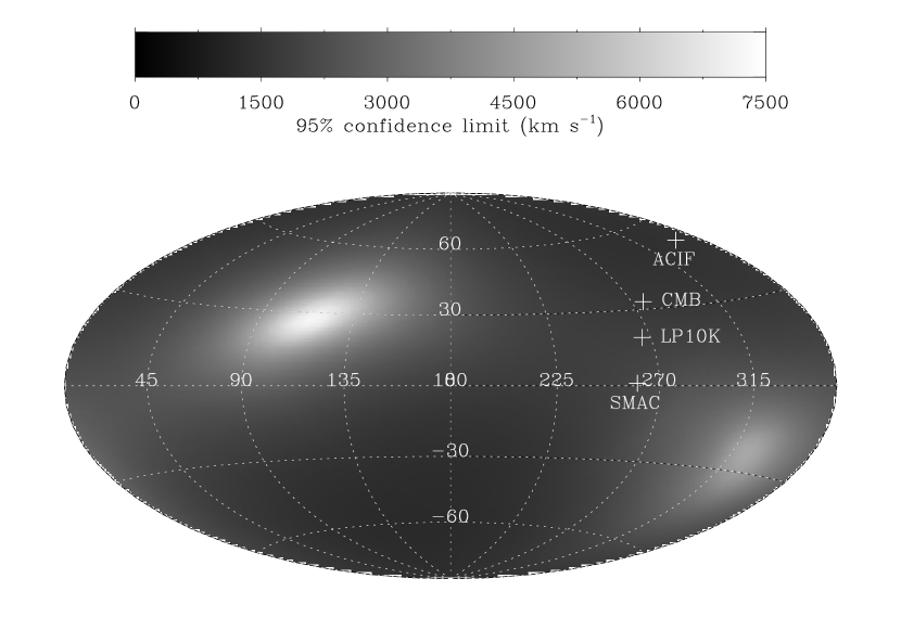
Figure 8: All-sky map showing the upper limit to dipole flow (95% confidence) as a function of location on the sky. The locations of the flows listed in Table Peculiar Velocity Limits from Measurements of the Spectrum of the Sunyaev-Zel’dovich Effect in Six Clusters of Galaxies are also shown.

where ${\bf V_{\rm B}}.\hat{r}$ is the component of the bulk flow in the direction of the ith cluster, and the likelihood of the flow, given the data, $L_{i}$, is determined from the SuZIE II data. In order to account for the effects of astrophysical confusion, we convolve the likelihood function for the peculiar velocity of each cluster with a gaussian probability with $\sigma=\pm 750$ km s^-1 before calculating the bulk-flow likelihood. As expected, we do not detect any bulk flow in our data. Figure 8 shows the 95% confidence limit to $V_{\rm B}$ as a function of location on the sky.

Because our clusters sparsely sample the peculiar velocity field, our upper limits are tighter in some directions than in others. For example, we have also used our data to set limits on bulk flows in the direction of the CMB dipole which is taken to have coordinates $(l,b)=(276^{\circ}\pm 3^{\circ},33^{\circ}\pm 3^{\circ})$ (Kogut et al., 1993). We find that at 95% confidence the flow in this direction is $\leq 1410$ km s^-1. The limits towards other directions for which optical measurements have yielded a flow detection are shown in Table Peculiar Velocity Limits from Measurements of the Spectrum of the Sunyaev-Zel’dovich Effect in Six Clusters of Galaxies.

8 Conclusions

We have used millimetric measurements of the SZ effect to set limits to the peculiar velocities of six galaxy clusters. By making measurements at three widely separated frequencies we have been able to separate the thermal and kinematic SZ spectra. Moreover, because our measurements in these bands are simultaneous, we have been able to discriminate and remove fluctuations in atmospheric emission which dominate the noise at these wavelengths. These observations have allowed us to make the first SZ-determined limits on bulk flows. In certain directions the limits are approaching the level of sensitivity achieved with optical surveys at much lower redshifts. Because our sky coverage is not uniform, our sensitivity to bulk flows varies greatly over the sky. We are continuing the SuZIE II observation program with the aim of obtaining a larger, more uniform cluster sample to improve our bulk flow limits.

The precision with which SuZIE II can measure peculiar velocities is limited not only by the small number of detectors, but also by atmospheric and instrumental noise, and astrophysical confusion from submillimeter galaxies. In the last few years the potential of SZ astronomy has been realized and new telescopes equipped with bolometer arrays that will have hundreds to thousands of pixels are planned (Carlstrom, Holder & Reese, 2002; Staggs & Church, 2001). Our measurements demonstrate the feasibility of using the SZ effect to measure cluster peculiar velocities, but highlight some issues that need further investigation:

1. The atmosphere will continue to be an issue for ground-based measurements. We have demonstrated that wide, simultaneous spectral coverage can significantly diminish, but not completely remove, this source of noise.

2. Confusion from submillimeter point sources can lead to a systematic peculiar velocity measurement. Further work is needed to determine the best strategy for identifying and removing this contaminant, especially for experiments that will map a large area of sky with lower angular resolution than SuZIE II, such as the High Frequency Instrument (HFI) that will operate at frequencies of 100–850 GHz as part of the Planck satellite (Lamarre et al., 2000). Although high-resolution measurements of clusters at millimeter wavelengths will be possible with future instruments such as ALMA, it may not be feasible to use this method to subtract astrophysical contamination from a sample of the size needed (of order 1000+ velocities) to effectively probe large-scale structure with SZ-determined peculiar velocities. Instruments such as SuZIE II will be invaluable for investigating removal techniques based on spectral rather than spatial information, especially if more frequency bands are incorporated into the instrument.

The SuZIE program is supported by a National Science Foundation grant AST-9970797 and by a Stanford Terman Fellowship awarded to SEC. JH acknowledges support from a National Science Foundation Graduate Research Fellowship and a Stanford Graduate Fellowship. This work was partially carried out at the Infrared Processing and Analysis Center and the Jet Propulsion Laboratory of the California Institute of Technology, under a contract with the National Aeronautics and Space Administration. We would like to thank the CSO staff for their assistance with SuZIE observations. The CSO is operated by the Caltech Submillimeter Observatory under contract from the National Science Foundation.

Appendix A Creating an Atmospheric Template

SuZIE makes simultaneous multi-frequency observations of a source. Besides the obvious advantage of instantaneously measuring the spectrum of the SZ source, this method permits atmospheric noise removal through spectral discrimination of the atmospheric signal. We realize this by creating an atmospheric template with no residual SZ signal for each row of photometers by forming a linear combination of the three differential frequency channels in that row on a scan by scan basis. We define this atmospheric template, $A_{j}(\theta)$, as:

$$A_{j}(\theta)=\alpha D_{1j}(\theta)+\gamma D_{2j}(\theta)+D_{3j}(\theta)$$ (A1)

where the coefficients $\alpha$ and $\gamma,$ are chosen to minimize the residual SZ signal in $A_{j}(\theta)$. If we define $F_{k}^{SZ}(\theta)$ as the SZ signal in channel $D_{k}(\theta)$ this implies that the residual SZ signal in our atmospheric template, which we define as $Z_{k}^{SZ}(\theta)$, is then

$$Z_{k}^{SZ}(\theta)=\alpha F_{1}^{SZ}(\theta)+\gamma F_{2}^{SZ}(\theta)+F_{3}^{SZ}(\theta)$$ (A2)

where the SZ flux in each channel includes contributions for both the thermal and kinematic effects, such that, $F_{k}^{SZ}(\theta)=F_{k}^{SZ,T}(\theta)+F_{k}^{SZ,K}(\theta)$. The thermal SZ flux in each channel, using the notation of §4.1, is more precisely:

$$F_{k}^{SZ,T}(\theta)=y_{0}\times T_{k}(T_{e})\times m_{k}(\theta)$$ (A3)

with $y_{0}$ being the central comptonization of the cluster, $T_{k}(T_{e})$ being defined in equation (13), and $m_{k}(\theta)$ defined in equation (12). Similarly, the kinematic SZ flux in each channel is

$$F_{k}^{SZ,K}(\theta)=y_{0}v_{p}\times K_{k}(T_{e})\times m_{k}(\theta)$$ (A4)

with $v_{p}$ being the peculiar velocity of the cluster, and $K_{k}(T_{e})$ defined in equation (14).

Using this notation we rewrite our expression for the residual SZ signal in the atmospheric template as

$$Z_{k}^{SZ}(\theta)=Z^{T}_{k}(\theta)+Z^{K}_{k}(\theta)$$ (A5)

with:

$$Z_{k}^{T}(\theta) = y_{0}\left[\alpha T_{1}(T_{e})m_{1}(\theta)+\gamma T_{2}(T_{e})m_{2}(\theta)+T_{3}(T_{e})m_{3}(\theta)\right]$$ (A6)

$$Z_{k}^{K}(\theta) = -y_{0}v_{p}\left[\alpha K_{1}(T_{e})m_{1}(\theta)+\gamma K_{2}(T_{e})m_{2}(\theta)+K_{3}(T_{e})m_{3}(\theta)\right]$$ (A7)

Solving for $Z_{k}^{SZ}(\theta)=0$ requires a position-dependent solution for $\alpha$ and $\gamma$ because $m_{k}(\theta)$ is not constant between frequency bands. For simplicity, we use the peak values of $m_{k}(\theta)$ to calculate $\alpha$ and $\gamma$ for $Z_{k}^{SZ}=0$. The error introduced from this assumption is discussed in Section 5.3.2. As an aside, this template should also be free of primary CMB anisotropy, on spatial scales similar to our clusters, because the kinematic SZ effect is spectrally indistinguishable from a primary CMB anisotropy.

Table 1: SuZIE Frequencies and Beam Sizes

	1996				1997-present
	$\nu_{0}$	$\Delta\nu$	FWHM	$\Omega$	$\nu_{0}$	$\Delta\nu$	FWHM	$\Omega$
Channel	[GHz]	[GHz]	arcmin	arcmin2	[GHz]	[GHz]	arcmin	arcmin2
270/350 GHz	$\cdots$	$\cdots$	$\cdots$	$\cdots$	$\cdots$	$\cdots$	$\cdots$	$\cdots$
$S^{+}_{10}$	274.0	32.6	1.35	1.85	355.1	30.3	1.50	2.17
$S^{-}_{10}$	272.8	28.8	1.30	1.79	354.2	31.1	1.54	2.42
$S^{+}_{11}$	272.9	30.3	1.25	1.65	356.7	30.8	1.57	2.24
$S^{-}_{11}$	272.3	30.6	1.30	1.76	354.5	31.5	1.60	2.58
221 GHz	$\cdots$	$\cdots$	$\cdots$	$\cdots$	$\cdots$	$\cdots$	$\cdots$	$\cdots$
$S^{+}_{20}$	222.2	22.4	1.30	1.64	221.4	21.8	1.36	1.90
$S^{-}_{20}$	220.0	23.1	1.25	1.67	220.5	23.8	1.40	2.08
$S^{+}_{21}$	220.7	24.8	1.15	1.53	221.7	22.9	1.47	2.02
$S^{-}_{21}$	220.0	24.1	1.20	1.54	220.8	21.7	1.40	2.18
145 GHz	$\cdots$	$\cdots$	$\cdots$	$\cdots$	$\cdots$	$\cdots$	$\cdots$	$\cdots$
$S^{+}_{30}$	146.1	19.9	1.45	2.14	145.2	18.1	1.50	2.35
$S^{-}_{30}$	146.4	21.3	1.40	2.16	144.6	18.6	1.64	2.73
$S^{+}_{31}$	145.0	20.7	1.30	1.86	145.5	18.2	1.60	2.51
$S^{-}_{31}$	144.4	19.5	1.35	1.91	144.9	17.4	1.60	2.73

Table 2: Summary of SuZIE observations

		R.A.	Decl.		Total	Accepted	Integration
Source	z	(J2000)	(J2000)	Date	Scans	Scans	Time (hours)	Ref.
A2261	0.22	17 22 27.6	$+$32 07 37.1	Mar 99	144	133	4.4	1
A2390	0.23	21 53 36.7	$+$17 41 43.7	Nov 00	147	128	4.3	1
ZW3146	0.29	10 23 38.8	$+$04 11 20.4	Nov 00	151	131	4.4	1
A1835	0.25	14 01 02.2	$+$02 52 43.0	Apr 96	638	577	19.2	1
Cl0016$+$16	0.55	00 21 08.5	$+$16 43 02.4	Nov 96	304	277	9.2	2
MS0451.6$-$0305	0.55	04 54 10.8	$-$03 00 56.8	Nov 96	405	348	11.6	2
′′				Nov 97	236	211	7.0
′′				Nov 00	375	306	10.2
MS0451.6$-$0305				Total	1016	865	28.8

References. — (1) Ebeling et al. (1998); (2) Gioia & Luppino (1994)

Table 3: Break down of the calibration uncertainties

Source	Uncertainty (%)
Detector non-linearities	6
Planetary temperature	6
Atmospheric $\tau$	2
Spectral response	1
Beam uncertainties	5
Total	10

Table 4: IC gas temperatures beta model parameters

	$kT_{e}$		$\theta_{c}$
Cluster	(keV)	$\beta$	(arcsec)	Ref.
A2261	$8.82^{+0.37}_{-0.32}$	$0.516^{+0.014}_{-0.013}$	$15.7^{+1.2}_{-1.1}$	1;2;2
A2390	$10.13^{+1.22}_{-0.99}$	$0.67^{+0.0}_{-0.0}$	$52.0^{+0.0}_{-0.0}$	1;3;3
Zw3146	$6.41^{+0.26}_{-0.25}$	$0.74^{+0.0}_{-0.0}$	$13.0^{+0.0}_{-0.0}$	1;3;3
A1835	$8.21^{0.19}_{-0.17}$	$0.595^{+0.007}_{-0.005}$	$12.2^{+0.6}_{-0.5}$	1;2;2
Cl0016	$7.55^{+0.72}_{-0.58}$	$0.749^{+0.024}_{-0.018}$	$42.3^{+2.4}_{-2.0}$	4;2;2
MS0451	$10.4^{+1.0}_{-0.8}$	$0.806^{+0.052}_{-0.043}$	$34.7^{+3.9}_{-3.5}$	5;2;2

References. — (1) Allen & Fabian (1998), (2) Reese et al. (2002), (3) Ettori & Fabian (1999), (4) Hughes & Birkinshaw (1998), (5) Donahue (1996)

Table 5: Differential Atmospheric Template Factors

Cluster	$\alpha$	$\gamma$
A2261	0.6366	-1.4490
A2390	0.6563	-1.4721
Zw3146	0.6428	-1.3808
MS0451 (Nov97)	0.6770	-1.3933
MS0451 (Nov00)	0.6449	-1.4286
$\cdots$	$\cdots$	$\cdots$
A1835	1.2133	-2.1745
Cl0016	1.2353	-2.2331
MS0451 (Nov96)	1.2246	-2.2076

Table 6: Summary of Results

Cluster	Date	$\Delta$ RA (arcsec)	$y_{0}\times 10^{4}$	$v_{pec}$ (km s-1)
A2261	Mar99	$1.3^{+11.0}_{-11.0}$	$7.58^{+2.24}_{-2.28}$	$-1400^{+1725}_{-1050}$
A2390	Nov00	$-2.5^{+14.3}_{-14.3}$	$1.67^{+1.03}_{-0.72}$	$+1950^{+6275}_{-2675}$
Zw3146	Nov00	$13.9^{+23.9}_{-22.9}$	$3.60^{+1.79}_{-2.61}$	$-650^{+3550}_{-1875}$
A1835	Apr96	$-22.5^{+12.0}_{-13.0}$	$7.54^{+1.61}_{-1.61}$	$-225^{+1650}_{-1225}$
Cl0016	Nov96	$-2.9^{+25.0}_{-26.9}$	$2.98^{+1.32}_{-2.59}$	$-4050^{+2900}_{-1775}$
MS0451	Nov96	$-1.5^{+16.0}_{-16.0}$	$2.09^{+1.87}_{-0.88}$	$+350^{+6625}_{-2925}$
$\cdots$	Nov97	$22.0^{+9.0}_{-9.0}$	$2.15^{+0.72}_{-0.73}$	$+1650^{+3775}_{-2125}$
$\cdots$	Nov00	$-25.0^{+17.0}_{-17.0}$	$3.06^{+0.83}_{-0.83}$	$-300^{+1950}_{-1250}$
$\cdots$	Combined Fit	$\cdots$	$2.80^{+0.51}_{-0.52}$	$+750^{+1500}_{-1125}$

Table 7: The Effects of Atmospheric Subtraction on Derived Fluxes for MS0451 Nov 2000 Data

Frequency	Flux (MJy sr-1)
(GHz)	With Atm. Subtraction	Without Atm. Subtraction
355	$0.547^{+0.159}_{-0.160}$	$-1.320^{+1.083}_{-1.084}$
221	$-0.055^{+0.077}_{-0.076}$	$-0.382^{+0.161}_{-0.162}$
145	$-0.228^{+0.040}_{-0.039}$	$-0.227^{+0.060}_{-0.060}$

Table 8: Effects of Calibration and IC Gas Model Uncertainties on MS0451 (Nov 2000)

Uncertainty	$y_{0}\times 10^{4}$	$v_{p}$ (km s-1)
string Statistical Uncertainty	$3.06^{+0.83}_{-0.83}$	$-300^{+1950}_{-1250}$
string Calibration (Absolute Only)	$3.02^{+0.84}_{-0.83}$	$-300^{+1950}_{-1250}$
string Calibration (Equal Absolute and Relative)	$3.02^{+0.83}_{-0.84}$	$-275^{+1950}_{-1250}$
string IC Density Model	$3.04^{+0.84}_{-0.83}$	$-300^{+1950}_{-1250}$
string IC Gas Temperature	$3.05^{+0.82}_{-0.82}$	$-275^{+1950}_{-1250}$

Table 9: SCUBA sources towards MS0451, A1835 and A2261.

		Source Coordinates		Flux (mJy)
Cluster	Source	RA (J2000)	Dec (J2000)	850$\mu$m	450$\mu$m	Ref.
A2261	SMMJ$17223+3207$	17 22 20.8	+32 07 04	$17.6\pm 3.9$	–	1
$\cdots$	$\cdots$	$\cdots$	$\cdots$	$\cdots$	$\cdots$
A1835	SMMJ$14009+0252$	14 00 57.7	+02 52 50	$14.5\pm 1.7$	$33\pm 7$	2
	SMMJ$14011+0252$	14 01 05.0	+02 52 25	$12.3\pm 1.7$	$42\pm 7$	2
	SMMJ$14010+0252$	14 01 02.3	+02 52 40	$5.4\pm 1.7$	$20\pm 7$	2
$\cdots$	$\cdots$	$\cdots$	$\cdots$	$\cdots$	$\cdots$
MS0451	SMMJ$04542-0301$	04 54 12.5	$-$03 01 04	$19.1\pm 4.2$	–	1

References. — (1) Chapman et al. (2002); (2) Smail et al. (2002)

Table 10: MS0451, A2261, and A1835 Sub-mm Galaxy Confusion

	Spectral	Flux/mJys					$v_{p}$
Cluster	Model	145GHz	221GHz	273GHz	355GHz	$y_{0}\times 10^{4}$	(km s-1)
MS0451	No Source	$-24.2^{+4.1}_{-4.1}$	$-5.4^{+6.7}_{-6.7}$	$\cdots$	$+55.4^{+15.8}_{-15.7}$	$3.06^{+0.83}_{-0.83}$	$-300^{+1950}_{-1250}$
	$\alpha=3$	$-24.9^{+4.1}_{-4.1}$	$-7.5^{+6.7}_{-6.7}$	$\cdots$	$+51.7^{+15.7}_{-15.8}$	$2.92^{+0.81}_{-0.83}$	$+25^{+2150}_{-1350}$
	$\alpha=2$	$-26.3^{+4.1}_{-4.1}$	$-9.5^{+6.7}_{-6.7}$	$\cdots$	$+49.4^{+15.8}_{-15.7}$	$2.87^{+0.81}_{-0.83}$	$+350^{+2275}_{-1425}$
$\cdots$	$\cdots$	$\cdots$	$\cdots$	$\cdots$	$\cdots$	$\cdots$
A2261	No Source	$-44.5^{+4.4}_{-4.4}$	$+11.0^{+14.1}_{-14.1}$	$\cdots$	$+113.9^{+29.7}_{-29.8}$	$7.58^{+2.24}_{-2.27}$	$-1400^{+1725}_{-1050}$
	$\alpha=3$	$-45.0^{+4.4}_{-4.4}$	$+8.9^{+14.1}_{-14.1}$	$\cdots$	$+110.0^{+29.8}_{-29.7}$	$7.37^{+2.20}_{-2.31}$	$-1250^{+1850}_{-1100}$
	$\alpha=2$	$-45.9^{+4.4}_{-4.4}$	$+7.9^{+14.1}_{-14.1}$	$\cdots$	$+108.9^{+29.8}_{-29.6}$	$7.34^{+2.20}_{-2.31}$	$-1150^{+1850}_{-1150}$
$\cdots$	$\cdots$	$\cdots$	$\cdots$	$\cdots$	$\cdots$	$\cdots$
A1835	No Source	$-36.3^{+5.6}_{-5.7}$	$+2.9^{+8.6}_{-8.6}$	$+38.2^{+12.6}_{-12.7}$	$\cdots$	$7.54^{+1.60}_{-1.61}$	$-200^{+1650}_{-1250}$
	$\alpha=3$	$-37.0^{+5.6}_{-5.7}$	$+0.9^{+8.6}_{-8.6}$	$+35.2^{+12.6}_{-12.7}$	$\cdots$	$7.29^{+1.61}_{-1.61}$	$+0^{+1750}_{-1300}$
	$\alpha=2$	$-38.0^{+5.7}_{-5.6}$	$-0.5^{+8.6}_{-8.6}$	$+33.6^{+12.7}_{-12.6}$	$\cdots$	$7.25^{+1.61}_{-1.61}$	$+100^{+1800}_{-1300}$
	$\alpha=1.7$	$-38.3^{+5.6}_{-5.7}$	$-1.0^{+8.6}_{-8.6}$	$+33.0^{+12.7}_{-12.6}$	$\cdots$	$7.25^{+1.61}_{-1.61}$	$+150^{+1800}_{-1300}$

Table 11: Comptonization and Peculiar Velocity Uncertainties for MS0451 (Nov 2000)

Uncertainty	$y_{0}\times 10^{4}$	$v_{p}$ (km s-1)
Statistical:	$3.06^{+0.83}_{-0.83}$	$-300^{+1950}_{-1250}$
Systematic:
string Common-Mode Atmospheric Removal	${}^{+0.06}_{-0.06}$	${}^{+10}_{-10}$
string Differential-Mode Atmospheric Removal	${}^{+0.01}_{-0.04}$	${}^{+50}_{-25}$
string Position Offset	${}^{+0.12}_{-0.00}$	${}^{+0}_{-0}$
string Primary Anisotropies	${}^{+0.05}_{-0.05}$	${}^{+380}_{-380}$
string Sub-millimeter Galaxies	${}^{+0.20}_{-0.20}$	${}^{+650}_{-650}$
Total:a	3.06${}^{+0.83}_{-0.83}$${}^{+0.25}_{-0.21}$	$-300^{+1950}_{-1250}$${}^{+755}_{-755}$

Note. — ^a The first number is the statistical uncertainty, the second is the systematic uncertainty

Table 12: The SuZIE sample of peculiar velocity measurements

		Peculiar Velocity	Galactic Coordinates		Distance
	Redshift	(km s-1)	$l$ (deg.)	$b$ (deg.)	($h^{-1}$ Mpc)
A1689	0.18	0$+170^{+805}_{-600}$	$313.39$	+$61.10$	0520
A2163	0.20	0$+490^{+1310}_{-790}$	00$6.75$	+$30.52$	0570
A2261	0.22	$-1400^{+1725}_{-1050}$	0$55.61$	+$31.86$	0630
A2390	0.23	$+1950^{+6275}_{-2675}$	0$73.93$	$-27.83$	0650
A1835	0.25	0$-225^{+1650}_{-1225}$	$340.38$	+$60.59$	0710
ZW3146	0.29	0$-650^{+3350}_{-1875}$	$239.39$	+$47.96$	0810
MS0451	0.55	0$+750^{+1500}_{-1125}$	$201.50$	$-27.32$	1440
0016	0.55	$-4050^{+2900}_{-1775}$	$112.55$	$-45.54$	1440

Table 13: Limits to bulk flows in specific directions.

	Direction (Gal.)		Velocity (km s-1)
Flow name	$l$ (deg.)	$b$ (deg.)	Best Fit	95% conf. limit	Ref.
CMB Dipole	276	+33	$+60\pm 690$0	1410	1
ACIF	343	+52	$+130\pm 510$ 0	1130	2
LP10K	272	+10	$+40\pm 930$ 0	1860	3
SMAC	260	+10	0$0\pm 980$	1930	4

References. — (1) Kogut et al. (1993), (2) Lauer & Postman (1994), (3) Willick (1999), (4) Hudson et al. (1999)

Figure 3: Results of the 2-d likelihood fit of the combined measurements of MS0451 in November 1996, 1997, and 2000. The 68.3% and 95.4% confidence regions are shown for peak Comptonization and peculiar velocity.

Figure 4: The measured spectrum for each cluster in the SuZIE II sample. In each plot the solid line is the best-fit SZ model, the dashed line is the thermal component of the SZ effect and the dotted line is the kinematic component of the SZ effect

Figure 5: Co-added scans of MS0451 from November 1997 for the on-source row for each of the three SuZIE frequency bands. The heavy line is the best-fit model to the co-added scan, while the lighter lines represent the 1-$\sigma$ uncertainty to those fits.

Figure 6: The measured spectra of MS0451 from each of the three observing runs as well as the combined spectra using the weighted mean of each spectral point. In each plot the solid line is the best-fit SZ model, the dashed line is the thermal component of the SZ effect and the dotted line is the kinematic component of the SZ effect.

Figure 7: Left: the stars denote the location, in galactic coordinates, of the clusters observed by SuZIE. The direction of the CMB dipole is also shown. Right: the measurements of the clusters plotted against redshift. The cross-hatched region shows the range that has been probed using optical measurements of peculiar velocities.

References

- Archibald et al. (2002) Archibald, E. N., Jenness, T., Holland, W. S., Coulson, I. M., Jessop, N. E., Stevens, J. A., Robson, E. I., Tilanus, R. P. J., Duncan, W. D., Lightfoot, J. F. 2002, MNRAS, 336, 1
- Allen & Fabian (1998) Allen, S.W., & Fabian, A.C., 1998, MNRAS, 297, L57
- Battistelli et al. (2002) Battistelli, E.S., De Petris, M., Lamagna, L., Melchiorri, F., Palladino, E., Savini, G., Cooray, A., Melchiorri, A., Rephaeli, Y., & Shimon, M. 2002, ApJ, 580, L101
- Blain et al. (2002) Blain, A. W., Smail, I., Ivison, R. J., Kneib, J.-P., & Frayer, D. T. 2002, Phys. Rep., 369, 111
- Branchini et al. (2000) Branchini, E., Zehavi, I., Plionis, M., & Dekel, A. 2000, MNRAS, 313, 491
- Bridle et al. (2001) Bridle, S. L., Zehavi, I., Dekel, A., Lahav, O., Hobson, M. P., & Lasenby, A. N. 2001, MNRAS, 321, 333
- Carlstrom, Holder & Reese (2002) Carlstrom, J. E., Holder, G.P., & Reese, E.D. 2002, ARA&A, 40 in press
- Cavaliere & Fusco-Femiano (1976) Cavaliere, A. & Fusco-Femiano, R. 1976, A&A, 49, 137
- Cavaliere & Fusco-Femiano (1978) Cavaliere, A. & Fusco-Femiano, R. 1978, A&A, 70, 677
- Challinor & Lasenby (1998) Challinor, A., & Lasenby, A., 1998, ApJ, 499, 1
- Chapman et al. (2002) Chapman, S.C., Scott, D., Borys, C., & Fahlman, G.G., 2002, MNRAS, 330, 92
- Colless et al. (2001) Colless, M., Saglia, R. P., Burstein, D., Davies, R. L., McMahan, R. K., & Wegner, G. 2001, MNRAS, 321, 277
- Courteau & Dekel (2001) Courteau, S. & Dekel, A. 2001, to appear in “Astrophysical Ages and Time Scales”, eds, T. von Hippel, N. Manset, C. Simpson (ASP Conf. Series), (astro-ph/0105470)
- Courteau, Strauss & Willick (2000) Courteau, S., Strauss, M.A., & Willick, J.A., eds., 2000, Cosmic Flows 1999: Towards an Understanding of Large-Scale Structure, ASP Conference Series
- Dale & Giovanelli (2000) Dale, D. A. & Giovanelli, R. 2000, ASP Conf. Ser. 201: Cosmic Flows Workshop, 25
- De Petris et al. (2002) De Petris, M., D Alba, L., Lamagna, L., Melchiorri, F., Orlando, A., Palladino, E., Rephaeli, Y., Colafrancesco, S., Kreysa, E., Signore, M. 2002, ApJ, 574, L119
- Dolgov et al. (2001) Dolgov, A. D., Hansen, S. H., Pastor, S., & Semikoz, D. V. 2001, ApJ, 554, 74
- Donahue (1996) Donahue, M., 1996, ApJ, 468, 79
- Doré, Knox & Peel (2002) Doré, O., Knox, L., Peel, A. 2002, ApJ submitted, (astroph/0207369)
- Ebeling et al. (1996a) Ebeling, H., Voges, W., Bohringer, H., Edge, A. C., Huchra, J. P., & Briel, U. G. 1996a, MNRAS, 281, 799
- Ebeling et al. (1996b) Ebeling, H., Voges, W., Bohringer, H., Edge, A. C., Huchra, J. P., & Briel, U. G. 1996b, MNRAS, 283, 1103
- Ebeling et al. (1998) Ebeling, H., Edge, A. C., Bohringer, H., Allen, S. W., Crawford, C. S., Fabian, A. C., Voges, W., & Huchra, J. P. 1998, MNRAS, 301, 881
- Ettori & Fabian (1999) Ettori, S., & Fabian, A.C., MNRAS, 305, 834
- Ganga et al. (1997) Ganga, K. M., Ratra, B., Church, S. E., Sugiyama, N., Ade, P. A. R., Holzapfel, W. L., Mauskopf, P. D., Wilbanks, T. M., and Lange, A. E. 1997, ApJ, 484, 517
- Gioia et al. (1990) Gioia, I. M., Maccacaro, T., Schild, R. E., Wolter, A., Stocke, J. T., Morris, S. L., & Henry, J. P. 1990, ApJS, 72, 567
- Gioia & Luppino (1994) Gioia, I. M. & Luppino, G. A. 1994, ApJS, 94, 583
- Goldin et al. (1997) Goldin, A.B., Kowitt, M.S., Cheng, E.S., Cottingham, D.A., Fixsen, D.J., Inman, C.A., Meyer, S.S., Puchalla, J.L., Ruhl, J.E., and Silverberg, R.F. 1997, ApJ, 488, L161 MNRAS, 333, 318
- Gramann et al. (1995) Gramann, M., Bahcall, N. A., Cen, R., & Gott, J. R. 1995, ApJ, 441, 449
- Grego et al. (2001) Grego , L., Carlstrom , J. E., Reese, E. D., Holder , G. P., Holzapfel, W. L., Joy, M. K., Mohr, J. J., & Patel, S. 2001, 552, 2
- Griffin & Orton (1993) Griffin, M.J., & Orton, G.S. 1993, Icarus, 105, 537
- Hansen, Pastor & Semikov (2002) Hansen, S. H., Pastor, S. & Semikoz, D. V. 2002, ApJ, 573, L69
- Holzapfel et al. (1997a) Holzapfel, W.L., Arnaud, M., Ade, P.A.R., Church, S.E., Fischer, M.L., Mauskopf, P.D., Rephaeli, Y., Wilbanks, T.M., and Lange, A.E. 1997a, ApJ, 480, 449
- Holzapfel et al. (1997b) Holzapfel, W.L., Ade, P.A.R., Church, S.E., Mauskopf, P.D., Rephaeli, Y., Wilbanks, T.M., and Lange, A.E. 1997b, ApJ, 481, 35
- Hughes & Birkinshaw (1998) Hughes, J.P., & Birkinshaw, M., 1998, ApJ, 501, 1
- Hudson et al. (1999) Hudson, M. J., Smith, R. J., Lucey, J. R., Schlegel, D. J., & Davies, R. L. 1999, ApJ, 512, L79
- Itoh et al. (1998) Itoh, N., Kohyama, Y., & Nozawa, S., 1998, ApJ, 502, 7
- Jones et al. (2001) Jones, M. E., Edge, A C., Grainge, K., Grainger, W. F., Kneissl, R., Pooley, G. G., Saunders, R., Miyoshi, S. J., Tsuruta, T., Yamashita, K., Tawara, Y., Furuzawa, A., Harada, A., Hatsukade, I. 2001, MNRAS, submitted, (astro-ph/0103046)
- Kompaneets (1957) Kompaneets, A.S., 1957, Soviet Physics JETP Lett, 4, 730
- Kogut et al. (1993) Kogut, A., et al. 1993, ApJ, 419, 1
- Lamarre et al. (2000) Lamarre, J. M. et al. 2000, Astrophysical Letters Communications, 37, 161
- LaRoque et al. (2002) LaRoque, S.L., Carlstrom, J.E., Reese, E.D., Holder, G.P., Holzapfel, W.L., Joy, M., and Grego, L. 2002, ApJ, submitted (astro-ph/0204134)
- Lauer & Postman (1994) Lauer, T. R. & Postman, M. 1994, ApJ, 425, 418
- Mauskopf et al. (2000) Mauskopf, P.D., Ade, P.A.R., Allen, S.W., Church, S.E., Edge, A.C., Ganga, K.M., Holzapfel, W.L., Lange, A.E., Rownd, B.K., Philhour, B.J., and Runyan, M.C. 2000, ApJ, 538, 505
- Mauskopf et al. (1997) Mauskopf, P.D., Bock, J.J., Del Castillo, H., Holzapfel, W.L., & Lange, A.E., 1997, Applied Optics, Vol. 36, No. 4, 765
- Myers et al. (1997) Myers S. T., Baker, J. E., Readhead, A. C. S., Leitch E. M., Herbig, T. 1997, ApJ, 485, 1
- Nozawa et al. (1998) Nozawa, S., Itoh, N., & Kohyama, Y., 1998, ApJ, 508, 17
- Peel & Knox (2002) Peel, A., & Knox, L. 2002, preprint, (astroph/0205438)
- Pointecouteau, Giard & Barret (1998) Pointecouteau, E., Giard, M., & Barret, D. 1998, A&A, 336, 44
- Pointecouteau et al. (1999) Pointecouteau, E., Giard, M., Benoit, A., Désert, F.X., Aghanim, N., Coron, N., Lamarre, J. M., & Delabrouille, J. 1999, ApJ, 519, L115
- Pointecouteau et al. (2001) Pointecouteau, E., Giard, M., Benoit, A., Désert, F.X., Bernard, J.P., Coron, N., & Lamarre, J. M. 2001, ApJ, 552, 42
- Press et al. (1992) Press, W.H., Teukolsky, S.A., Vetterling, W.T., & Flannery, B.P., 1992, Numerical Recipes in C (New York: Cambridge Univ. Press)
- Reese et al. (2000) Reese, E.D., Mohr, J.J., Carlstrom, J.E., Joy, M., Grego, L., Holder, G.P., Holzapfel, W.L., Hughes, J.P., Patel, S.K., & Donahue, M., 2000, ApJ, 533, 38
- Reese et al. (2002) Reese, E. D., Carlstrom, J. E., Joy, M., Mohr, J. J., Grego, L., & Holzapfel, W. L. 2002, ApJ, 581, 53
- Rephaeli (1980) Rephaeli Y. 1980, ApJ, 241, 858
- Rephaeli (1995) Rephaeli, Y. 1995, ApJ, 445, 33
- Sheth & Diaferio (2001) Sheth, R.K, & Diaferio, A. 2001, MNRAS, 322, 901
- Shimon & Rephaeli (2002) Shimon, M. & Rephaeli, Y. 2002, ApJ, 575, 12
- Smail et al. (2002) Smail, I., Ivision, R.J., Blain, A.W., & Kneib, J.P., 2002, MNRAS, 331, 495
- Staggs & Church (2001) Staggs, S., & Church, S. 2001, Proc. of the APS/DPF/DPB Summer Study on the Future of Particle Physics (Snowmass 2001) ed. N. Graf, (astro-ph/0111576)
- Strauss & Willick (1995) Strauss, M.A., & Willick, J.A., 1995, Physics Reports, 261, 271
- Suhhonenko & Gramann (2002) Suhhonenko, I., & Gramann, M. 2002, MNRAS submitted, (astroph/0203166)
- Sunyaev & Zel’dovich (1972) Sunyaev, R.A., & Zel’dovich, Ya. B. 1972, Comments Astrophys. Space Phys., 4, 173
- Sunyeav & Zel’dovich (1980) Sunyeav, R.A., & Zel’dovich, Ya. B. 1980, MNRAS, 190, 413
- Willick (1999) Willick, J. A. 1999, ApJ, 522, 647