Cosmology from Topological Defects

Abstract

The potential role of cosmic topological defects has raised interest in the astrophysical community for many years now. In this set of notes, we give an introduction to the subject of cosmic topological defects and some of their possible observable signatures. We begin with a review of the basics of general defect formation and evolution, we briefly comment on some general features of conducting cosmic strings and vorton formation, as well as on the possible role of defects as dark energy, to end up with cosmic structure formation from defects and some specific imprints in the cosmic microwave background radiation from simulated cosmic strings. A detailed, pedagogical explanation of the mechanism underlying the tiny level of polarization discovered in the cosmic microwave background by the DASI collaboration (and recently confirmed by WMAP) is also given, and a first rough comparison with some predictions from defects is provided.

I Introduction

On a cold day, ice forms quickly on the surface of a pond. But it does not grow as a smooth, featureless covering. Instead, the water begins to freeze in many places independently, and the growing plates of ice join up in random fashion, leaving zig–zag boundaries between them. These irregular margins are an example of what physicists call “topological defects” – defects because they are places where the crystal structure of the ice is disrupted, and topological because an accurate description of them involves ideas of symmetry embodied in topology, the branch of mathematics that focuses on the study of continuous surfaces.

Current theories of particle physics likewise predict that a variety of topological defects would almost certainly have formed during the early evolution of the universe. Just as water turns to ice (a phase transition) when the temperature drops, so the interactions between elementary particles run through distinct phases as the typical energy of those particles falls with the expansion of the universe. When conditions favor the appearance of a new phase, it generally crops up in many places at the same time, and when separate regions of the new phase run into each other, topological defects are the result. The detection of such structures in the modern universe would provide precious information on events in the earliest instants after the Big Bang. Their absence, on the other hand, would force a major revision of current physical theories.

The aim of this set of Lectures is to introduce the reader to the subject of cosmology from topological defects. We begin with a review of the basics of defect formation and evolution, to get a grasp of the overall picture. We will see that defects are generically predicted to exist in most interesting models of high energy physics trying to describe the early universe. The basic elements of the standard cosmology, with its successes, shortcomings, and new developments, are covered elsewhere in this volume. See for example the lecture notes by Rocky Kolb on Astroparticle Physics, Ed Copeland’s material on String / M-Theory Cosmology, and Jim Bartlett’s Observational Cosmology. So we will not devote much space to these topics here. Rather, we will focus on some specific subjects. We will first briefly comment on conducting cosmic strings and one of their most important predictions for cosmology, namely, the existence of equilibrium configurations of string loops, dubbed vortons. We will then pass on to study some key signatures that a network of defects would produce on the cosmic microwave background (CMB) radiation, e.g., the CMB bispectrum of the temperature anisotropies from a simulated model of cosmic strings. Miscellaneous topics also reviewed below are, for example, the way in which these cosmic entities lead to large–scale structure formation and some astrophysical footprints left by the various defects, and we will discuss the possibility of isolating their effects by astrophysical observations. Also, we include a short, detailed discussion of CMB polarization and some brief comparison with the predictions from cosmic defects.

Many areas of modern research directly related to cosmic defects are unfortunately not covered in these notes. The subject is now so vast -and beyond the possibilities of a single review- that we suggest the reader to consult some of the excellent recent literature already available. So, have a look, for example, to the report by Achúcarro & Vachaspati [2000] for a treatment of semilocal and electroweak strings , and to [Vachaspati, 2001] for a review of certain topological defects, like monopoles, domain walls and, again, electroweak strings, virtually not covered here. For conducting defects, cosmic strings in particular, see for example [Gangui & Peter, 1998] for a brief overview of many different astrophysical and cosmological phenomena, [Gangui, 2001b], from which this review borrows (and updates) a great deal of material, for a treatment of conducting cosmic strings and one of their most important predictions for cosmology, namely, the existence of equilibrium configurations of string loops, dubbed vortons. Finally, refer to the comprehensive colorful lecture notes by Carter [1997] on the dynamics of branes with applications to conducting cosmic strings and vortons. If your are in cosmological structure formation, Durrer [2000] presents a good review of modern developments on global topological defects and their relation to CMB anisotropies, while Magueijo & Brandenberger [2000] give a set of imaginative lectures with an update on local string models of large-scale structure formation and also baryogenesis with cosmic defects. Finally, Durrer, Kunz & Melchiorri [2002] give a complete update of cosmic structure formation with global defects, including detailed analyses of correlators, mixed models, and the resulting matter and CMB power spectra.

The interdisciplinary subject of topological defects in the cosmos and the lab is nicely covered in the proceedings of the school held aux Houches on topological defects and non-equilibrium dynamics, edited by Bunkov & Godfrin [2000]; the ensemble of lectures in this volume, together with the recent review by Kibble [2002], give an exhaustive illustration of this fast developing area of research, which includes various fields of physics, like low–temperature condensed–matter, liquid crystals, astrophysics and high–energy physics. Finally, all of the above can also be found in the concise review by Hindmarsh & Kibble [1995], particularly concerned with the physics and cosmology of cosmic strings, and in the monograph by Vilenkin & Shellard [2000] on cosmic strings and other topological defects.

I.1 How defects form

A central concept of particle physics theories attempting to unify all the fundamental interactions is the concept of symmetry breaking. As the universe expanded and cooled, first the gravitational interaction, and subsequently all other known forces would have begun adopting their own identities. In the context of the standard hot Big Bang theory the spontaneous breaking of fundamental symmetries is realized as a phase transition in the early universe. Such phase transitions have several exciting cosmological consequences and thus provide an important link between particle physics and cosmology.

There are several symmetries which are expected to break down in the course of time. In each of these transitions the space–time gets ‘oriented’ by the presence of a hypothetical force field called the ‘Higgs field’, named for Peter Higgs, pervading all the space. This field orientation signals the transition from a state of higher symmetry to a final state where the system under consideration obeys a smaller group of symmetry rules. As an every–day analogy we may consider the transition from liquid water to ice; the formation of the crystal structure ice (where water molecules are arranged in a well defined lattice), breaks the symmetry possessed when the system was in the higher temperature liquid phase, when every direction in the system was equivalent. In the same way, it is precisely the orientation in the Higgs field which breaks the highly symmetric state between particles and forces.

Having built a model of elementary particles and forces, particle physicists and cosmologists are today embarked on a difficult search for a theory that unifies all the fundamental interactions. As we mentioned, an essential ingredient in all major candidate theories is the concept of symmetry breaking. Experiments have determined that there are four physical forces in nature; in addition to gravity these are called the strong, weak and electromagnetic forces. Close to the singularity of the hot Big Bang, when energies were at their highest, it is believed that these forces were unified in a single, all–encompassing interaction. As the universe expanded and cooled, first the gravitational interaction, then the strong interaction, and lastly the weak and the electromagnetic forces would have broken out of the unified scheme and adopted their present distinct identities in a series of symmetry breakings.

Theoretical physicists are still struggling to understand how gravity can be united with the other interactions, but for the unification of the strong, weak and electromagnetic forces plausible theories exist. Indeed, force–carrying particles whose existence demonstrated the fundamental unification of the weak and electromagnetic forces into a primordial “electroweak” force – the W and Z bosons – were discovered at CERN, the European accelerator laboratory, in 1983. In the context of the standard Big Bang theory, cosmological phase transitions are produced by the spontaneous breaking of a fundamental symmetry, such as the electroweak force, as the universe cools. For example, the electroweak interaction broke into the separate weak and electromagnetic forces when the observable universe was $10^{-12}$ seconds old, had a temperature of $10^{15}$ degrees Kelvin, and was only one part in $10^{15}$ of its present size. There are also other phase transitions besides those associated with the emergence of the distinct forces. The quark-hadron confinement transition, for example, took place when the universe was about a microsecond old. Before this transition, quarks – the particles that would become the constituents of the atomic nucleus – moved as free particles; afterward, they became forever bound up in protons, neutrons, mesons and other composite particles.

As we said, the standard mechanism for breaking a symmetry involves the hypothetical Higgs field that pervades all space. As the universe cools, the Higgs field can adopt different ground states, also referred to as different vacuum states of the theory. In a symmetric ground state, the Higgs field is zero everywhere. Symmetry breaks when the Higgs field takes on a finite value (see Figure 1).

Figure 1: Temperature–dependent effective potential for a first–order phase transition for the Higgs field. For very high temperatures, well above the critical one $T_{c}$, the potential possesses just one minimum for the vanishing value of the Higgs field. Then, when the temperature decreases, a whole set of minima develops (it may be two or more, discrete or continuous, depending of the type of symmetry under consideration). Below $T_{c}$, the value $\phi=0$ stops being the global minimum and the system will spontaneously choose a new (lower) one, say $\phi=\eta\exp(i\theta)$ (for complex $\phi$) for some angle $\theta$ and nonvanishing $\eta$, amongst the available ones. This choice signals the breakdown of the symmetry in a cosmic phase transition and the generation of random regions of conflicting field orientations $\theta$. In a cosmological setting, the merging of these domains gives rise to cosmic defects.

Kibble [1976] first saw the possibility of defect formation when he realized that in a cooling universe phase transitions proceed by the formation of uncorrelated domains that subsequently coalesce, leaving behind relics in the form of defects. In the expanding universe, widely separated regions in space have not had enough time to ‘communicate’ amongst themselves and are therefore not correlated, due to a lack of causal contact. It is therefore natural to suppose that different regions ended up having arbitrary orientations of the Higgs field and that, when they merged together, it was hard for domains with very different preferred directions to adjust themselves and fit smoothly. In the interfaces of these domains, defects form. Such relic ‘flaws’ are unique examples of incredible amounts of energy and this feature attracted the minds of many cosmologists.

I.2 Phase transitions and finite temperature field theory

Phase transitions are known to occur in the early universe. Examples we mentioned are the quark to hadron (confinement) transition, which QCD predicts at an energy around 1 GeV, and the electroweak phase transition at about 250 GeV. Within grand unified theories (GUT), aiming to describe the physics beyond the standard model, other phase transitions are predicted to occur at energies of order $10^{15}$ GeV; during these, the Higgs field tends to fall towards the minima of its potential while the overall temperature of the universe decreases as a consequence of the expansion.

A familiar theory to make a bit more quantitative the above considerations is the $\lambda|\phi|^{4}$ theory,

$${\cal L}={1\over 2}|\partial_{\mu}\phi|^{2}+{1\over 2}m_{0}^{2}|\phi|^{2}-{\lambda\over 4!}|\phi|^{4}~{},$$ (1)

with $m^{2}_{0}>0$. The second and third terms on the right hand side yield the usual ‘Mexican hat’ potential for the complex scalar field. For energies much larger than the critical temperature, $T_{c}$, the fields are in the so–called ‘false’ vacuum: a highly symmetric state characterized by a vacuum expectation value $\bigl{\langle}|\phi|\bigr{\rangle}=0$. But when energies decrease the symmetry is spontaneously broken: a new ‘true’ vacuum develops and the scalar field rolls down the potential and sits onto one of the degenerate new minima. In this situation the vacuum expectation value becomes $\bigl{\langle}|\phi|\bigr{\rangle}^{2}=6m_{0}^{2}/\lambda$.

Research done in the 1970’s in finite–temperature field theory [Weinberg, 1974; Dolan & Jackiw, 1974; Kirzhnits & Linde, 1974] has led to the result that the temperature–dependent effective potential can be written down as

$$V_{T}(|\phi|)=-{1\over 2}m^{2}(T)|\phi|^{2}+{\lambda\over 4!}|\phi|^{4}$$ (2)

with $T_{c}^{2}=24m_{0}^{2}/\lambda$, $m^{2}(T)=m_{0}^{2}(1-T^{2}/T_{c}^{2})$, and $\bigl{\langle}|\phi|\bigr{\rangle}^{2}=6m^{2}(T)/\lambda$. We easily see that when $T$ approaches $T_{c}$ from below the symmetry is restored, and again we have $\bigl{\langle}|\phi|\bigr{\rangle}=0$. In condensed–matter jargon, the transition described above is second–order [Mermin, 1979].

I.3 The Kibble mechanism

The model described in the last subsection is an example in which the transition may be second–order. As we saw, for temperatures much larger than the critical one the vacuum expectation value of the scalar field vanishes at all points of space, whereas for $T<T_{c}$ it evolves smoothly in time towards a non vanishing $\bigl{\langle}|\phi|\bigr{\rangle}$. Both thermal and quantum fluctuations influence the new value taken by $\bigl{\langle}|\phi|\bigr{\rangle}$ and therefore it has no reasons to be uniform in space. This leads to the existence of domains wherein the $\bigl{\langle}|\phi(\vec{x})|\bigr{\rangle}$ is coherent and regions where it is not. The consequences of this fact are the subject of this subsection.

Phase transitions can also be first–order proceeding via bubble nucleation. At very high energies the symmetry breaking potential has $\bigl{\langle}|\phi|\bigr{\rangle}=0$ as the only vacuum state. When the temperature goes down to $T_{c}$ a set of vacua, degenerate to the previous one, develops. However this time the transition is not smooth as before, for a potential barrier separates the old (false) and the new (true) vacua (see, e.g. Figure 1). Provided the barrier at this small temperature is high enough, compared to the thermal energy present in the system, the field $\phi$ will remain trapped in the false vacuum state even for small ($<T_{c}$) temperatures. Classically, this is the complete picture. However, quantum tunneling effects can liberate the field from the old vacuum state, at least in some regions of space: there is a probability per unit time and volume in space that at a point $\vec{x}$ a bubble of true vacuum will nucleate. The result is thus the formation of bubbles of true vacuum with the value of the field in each bubble being independent of the value of the field in all other bubbles. This leads again to the formation of domains where the fields are correlated, whereas no correlation exits between fields belonging to different domains. Then, after creation the bubble will expand at the speed of light surrounded by a ‘sea’ of false vacuum domains. As opposed to second–order phase transitions, here the nucleation process is extremely inhomogeneous and $\bigl{\langle}|\phi(\vec{x})|\bigr{\rangle}$ is not a continuous function of time.

Let us turn now to the study of correlation lengths and their rôle in the formation of topological defects. One important feature in determining the size of the domains where $\bigl{\langle}|\phi(\vec{x})|\bigr{\rangle}$ is coherent is given by the spatial correlation of the field $\phi$. Simple field theoretic considerations [see, e.g., Copeland, 1993] for long wavelength fluctuations of $\phi$ lead to different functional behaviors for the correlation function $G(r)\equiv\bigl{\langle}\phi(r_{1})\phi(r_{2})\bigr{\rangle}$, where we noted $r=|r_{1}-r_{2}|$. What is found depends radically on whether the wanted correlation is computed between points in space separated by a distance $r$ much smaller or much larger than a characteristic length $\xi^{-1}=m(T)\simeq\sqrt{\lambda}~{}|\bigl{\langle}\phi\bigr{\rangle}|$, known as the correlation length. Then, we have $G(r)\simeq{T_{c}\over 4\pi r}\exp(-{r\over\xi})$ for $r>>\xi$ , while $G(r)\simeq{T^{2}\over 2\pi^{2}}$ for $r<<\xi$ .

This tells us that domains of size $\xi\sim m^{-1}$ arise where the field $\phi$ is correlated. On the other hand, well beyond $\xi$ no correlations exist and thus points separated apart by $r>>\xi$ will belong to domains with in principle arbitrarily different orientations of the Higgs field. This in turn leads, after the merging of these domains in a cosmological setting, to the existence of defects, where field configurations fail to match smoothly.

However, when $T\to T_{c}$ we have $m\to 0$ and so $\xi\to\infty$, suggesting perhaps that for all points of space the field $\phi$ becomes correlated. This fact clearly violates causality. The existence of particle horizons in cosmological models (proportional to the inverse of the Hubble parameter $H^{-1}$) constrains microphysical interactions over distances beyond this causal domain. Therefore we get an upper bound to the correlation length as $\xi<H^{-1}\sim t$.

The general feature of the existence of uncorrelated domains has become known as the Kibble mechanism [Kibble, 1976] and it seems to be generic to most types of phase transitions.

I.4 A survey of topological defects

Different models for the Higgs field lead to the formation of a whole variety of topological defects, with very different characteristics and dimensions. Some of the proposed theories have symmetry breaking patterns leading to the formation of ‘domain walls’ (mirror reflection discrete symmetry): incredibly thin planar surfaces trapping enormous concentrations of mass–energy which separate domains of conflicting field orientations, similar to two–dimensional sheet–like structures found in ferromagnets. Within other theories, cosmological fields get distributed in such a way that the old (symmetric) phase gets confined into a finite region of space surrounded completely by the new (non–symmetric) phase. This situation leads to the generation of defects with linear geometry called ‘cosmic strings’. Theoretical reasons suggest these strings (vortex lines) do not have any loose ends in order that the two phases not get mixed up. This leaves infinite strings and closed loops as the only possible alternatives for these defects to manifest themselves in the early universe.

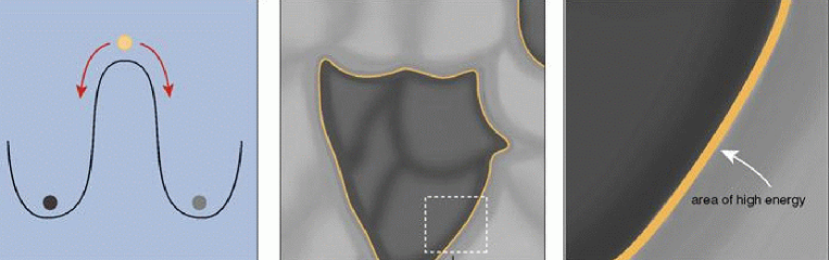
Figure 2: In a simple model of symmetry breaking, the initial symmetric ground state of the Higgs field (yellow central dot) can fall into the left- or right-hand valley of a double-well energy potential (light and dark dots). In a cosmic phase transition, regions of the new phase appear randomly and begin to grow and eventually merge as the transition proceeds toward completion (middle). Regions in which the symmetry has broken the same way can coalesce, but where regions that have made opposite choices encounter each other, a topological defect known as a domain wall forms (right). Across the wall, the Higgs field has to go from one of the valleys to the other (in the left panel), and must therefore traverse the energy peak. This creates a narrow planar region of very high energy, in which the symmetry is locally unbroken.

With a bit more abstraction scientists have even conceived other (semi) topological defects, called ‘textures’. These are conceptually simple objects, yet, it is not so easy to imagine them for they are just global field configurations living on a three–sphere vacuum manifold (the minima of the effective potential energy), whose non linear evolution perturbs spacetime. Turok [1989] was the first to realize that many unified theories predicted the existence of peculiar Higgs field configurations known as (texture) knots, and that these could be of potential interest for cosmology. Several features make these defects interesting. In contrast to domain walls and cosmic strings, textures have no core and thus the energy is more evenly distributed over space. Secondly, they are unstable to collapse and it is precisely this last feature which makes these objects cosmologically relevant, for this instability makes texture knots shrink to a microscopic size, unwind and radiate away all their energy. In so doing, they generate a gravitational field that perturbs the surrounding matter in a way which can seed structure formation.

I.5 Conditions for their existence: topological criteria

Let us now explore the conditions for the existence of topological defects. It is widely accepted that the final goal of particle physics is to provide a unified gauge theory comprising strong, weak and electromagnetic interactions (and some day also gravitation). This unified theory is to describe the physics at very high temperatures, when the age of the universe was slightly bigger than the Planck time. At this stage, the universe was in a state with the highest possible symmetry, described by a symmetry group G, and the Lagrangian modeling the system of all possible particles and interactions present should be invariant under the action of the elements of G.

As we explained before, the form of the finite temperature effective potential of the system is subject to variations during the cooling down evolution of the universe. This leads to a chain of phase transitions whereby some of the symmetries present in the beginning are not present anymore at lower temperatures. The first of these transitions may be described as G$\to$H, where now H stands for the new (smaller) unbroken symmetry group ruling the system. This chain of symmetry breakdowns eventually ends up with SU(3)$\times$SU(2)$\times$U(1), the symmetry group underlying the ‘standard model’ of particle physics.

A broken symmetry system (with a Mexican-hat potential for the Higgs field) may have many different minima (with the same energy), all related by the underlying symmetry. Passing from one minimum to another is included as one of the symmetries of the original group G, and the system will not change due to one such transformation. If a certain field configuration yields the lowest energy state of the system, transformations of this configuration by the elements of the symmetry group will also give the lowest energy state. For example, if a spherically symmetric system has a certain lowest energy value, this value will not change if the system is rotated.

The system will try to minimize its energy and will spontaneously choose one amongst the available minima. Once this is done and the phase transition achieved, the system is no longer ruled by G but by the symmetries of the smaller group H. So, if G$\to$H and the system is in one of the lowest energy states (call it $S_{1}$), transformations of $S_{1}$ to $S_{2}$ by elements of G will leave the energy unchanged. However, transformations of $S_{1}$ by elements of H will leave $S_{1}$ itself (and not just the energy) unchanged. The many distinct ground states of the system $S_{1},S_{2},\ldots$ are given by all transformations of G that are not related by elements in H. This space of distinct ground states is called the vacuum manifold and denoted $\cal M$. So, $\cal M$ is the space of all elements of G in which elements related by transformations in H have been identified. Mathematicians call it the coset space and denote it G$/$H. We then have ${\cal M}=$ G$/$H.

The importance of the study of the vacuum manifold lies in the fact that it is precisely the topology of ${\cal M}$ what determines the type of defect that will arise. Homotopy theory tells us how to map ${\cal M}$ into physical space in a non–trivial way, and what ensuing defect will be produced. For instance, the existence of non contractible loops in ${\cal M}$ is the requisite for the formation of cosmic strings. In formal language this comes about whenever we have the first homotopy group $\pi_{1}({\cal M})\neq$ 1, where 1 corresponds to the trivial group. If the vacuum manifold is disconnected we then have $\pi_{0}({\cal M})\neq$ 1, and domain walls are predicted to form in the boundary of these regions where the field $\phi$ is away from the minimum of the potential. Analogously, if $\pi_{2}({\cal M})\neq$ 1 it follows that the vacuum manifold contains non contractible two–spheres, and the ensuing defect is a monopole. Textures arise when ${\cal M}$ contains non contractible three–spheres and in this case it is the third homotopy group, $\pi_{3}({\cal M})$, the one that is non trivial. We summarize this in Table 1 .

$\pi_{0}({\cal M})\neq$1	${\cal M}$ disconnected	Domain Walls
$\pi_{1}({\cal M})\neq$1	non contractible loops in ${\cal M}$	Cosmic Strings
$\pi_{2}({\cal M})\neq$1	non contractible 2–spheres in ${\cal M}$	Monopoles
$\pi_{3}({\cal M})\neq$1	non contractible 3–spheres in ${\cal M}$	Textures

Table 1: The topology of ${\cal M}$ determines the type of defect that will arise.

II Defects in the universe

Generically topological defects will be produced if the conditions for their existence are met. Then for example if the unbroken group H contains a disconnected part, like an explicit U(1) factor (something that is quite common in many phase transition schemes discussed in the literature), monopoles will be left as relics of the transition. This is due to the fundamental theorem on the second homotopy group of coset spaces [Mermin, 1979], which states that for a simply–connected covering group G we have

$$\pi_{2}({\bf G}/{\bf H})\cong\pi_{1}({\bf H}_{0})~{},$$ (3)

with ${\bf H}_{0}$ being the component of the unbroken group connected to the identity. Then we see that since monopoles are associated with unshrinkable surfaces in G$/$H, the previous equation implies their existence if H is multiply–connected. The reader may guess what the consequences are for GUT phase transitions: in grand unified theories a semi–simple gauge group G is broken in several stages down to H = SU(3)$\times$U(1). Since in this case $\pi_{1}({\bf H})\cong{\cal Z}$, the integers, we have $\pi_{2}({\bf G}/{\bf H})\neq$ 1 and therefore gauge monopole solutions exist [Preskill, 1979].

II.1 Local and global monopoles and domain walls

Monopoles are yet another example of stable topological defects. Their formation stems from the fact that the vacuum expectation value of the symmetry breaking Higgs field has random orientations ($\bigl{\langle}\phi^{a}\bigr{\rangle}$ pointing in different directions in group space) on scales greater than the horizon. One expects therefore to have a probability of order unity that a monopole configuration will result after the phase transition (cf. the Kibble mechanism). Thus, about one monopole per Hubble volume should arise and we have for the number density $n_{monop}\sim 1/H^{-3}\sim T_{c}^{6}/m_{P}^{3}$, where $T_{c}$ is the critical temperature and $m_{P}$ is Planck mass, when the transition occurs. We also know the entropy density at this temperature, $s\sim T_{c}^{3}$, and so the monopole to entropy ratio is $n_{monop}/s\simeq 100(T_{c}/m_{P})^{3}$. In the absence of non–adiabatic processes after monopole creation this constant ratio determines their present abundance. For the typical value $T_{c}\sim 10^{14}$ GeV we have $n_{monop}/s\sim 10^{-13}$. This estimate leads to a present $\Omega_{monop}h^{2}\simeq 10^{11}$, for the superheavy monopoles $m_{monop}\simeq 10^{16}$ GeV that are created. This value contradicts standard cosmology and the presently most attractive way out seems to be to allow for an early period of inflation: the massive entropy production will hence lead to an exponential decrease of the initial $n_{monop}/s$ ratio, yielding $\Omega_{monop}$ consistent with observations. In summary, the broad–brush picture one has in mind is that of a mechanism that could solve the monopole problem by ‘weeping’ these unwanted relics out of our sight, to scales much bigger than the one that will eventually become our present horizon today.

Note that these arguments do not apply for global monopoles as these (in the absence of gauge fields) possess long–range forces that lead to a decrease of their number in comoving coordinates. The large attractive force between global monopoles and antimonopoles leads to a high annihilation probability and hence monopole over–production does not take place. Simulations performed by Bennett & Rhie [1990] showed that global monopole evolution rapidly settles into a scale invariant regime with only a few monopoles per horizon volume at all times.

Given that global monopoles do not represent a danger for cosmology one may proceed in studying their observable consequences. The gravitational fields of global monopoles may lead to matter clustering and CMB anisotropies. Given an average number of monopoles per horizon of $\sim 4$, Bennett & Rhie [1990] estimate a scale invariant spectrum of fluctuations $(\delta\rho/\rho)_{H}\sim 30G\eta^{2}$ at horizon crossing. In a subsequent paper they simulate the large–scale CMB anisotropies and, upon normalization with COBE–DMR, they get roughly $G\eta^{2}\sim 6\times 10^{-7}$ in agreement with a GUT energy scale $\eta$ [Bennett & Rhie, 1993]. However, as we will see in the CMB sections below, current estimates for the angular power spectrum of global defects do not match the most recent observations, their main problem being the lack of power on the degree angular scale once the spectrum is normalized to COBE on large scales [Durrer et al., 1996; Durrer et al., 2002].

Let us concentrate now on domain walls, and briefly try to show why they are not welcome in any cosmological context [at least in the simple version we here consider – there is always room for more complicated (and contrived) models]. If the symmetry breaking pattern is appropriate at least one domain wall per horizon volume will be formed. The mass per unit surface of these two-dimensional objects is given by $\sim\lambda^{1/2}\eta^{3}$, where $\lambda$ as usual is the coupling constant in the symmetry breaking potential for the Higgs field. Domain walls are generally horizon–sized and therefore their mass is given by $\sim\lambda^{1/2}\eta^{3}H^{-2}$. This implies a mass energy density roughly given by $\rho_{DW}\sim\eta^{3}t^{-1}$ and we may readily see now how the problem arises: the critical density goes as $\rho_{crit}\sim t^{-2}$ which implies $\Omega_{DW}(t)\sim(\eta/m_{P})^{2}\eta t$. Taking a typical GUT value for $\eta$ we get $\Omega_{DW}(t\sim 10^{-35}{\rm sec})\sim 1$ already at the time of the phase transition. It is not hard to imagine that today this will be at variance with observations; in fact we get $\Omega_{DW}(t\sim 10^{18}{\rm sec})\sim 10^{52}$. This indicates that models where domain walls are produced are tightly constrained, and the general feeling is that it is best to avoid them altogether [see Kolb & Turner, 1990 for further details; see also Dvali et al., 1998, Pogosian & Vachaspati, 2000 and Alexander et al., 1999 for an alternative solution].

II.2 Are defects inflated away?

It is important to realize the relevance that the Kibble’s mechanism has for cosmology; nearly every sensible grand unified theory (with its own symmetry breaking pattern) predicts the existence of defects. We know that an early era of inflation helps in getting rid of the unwanted relics. One could well wonder if the very same Higgs field responsible for breaking the symmetry would not be the same one responsible for driving an era of inflation, thereby diluting the density of the relic defects. This would get rid not only of (the unwanted) monopoles and domain walls but also of any other (cosmologically appealing) defect. Let us follow [Brandenberger, 1993] and sketch why this actually does not occur. Take first the symmetry breaking potential of Eq. (2) at zero temperature and add to it a harmless $\phi$–independent term $3m^{4}/(2\lambda)$. This will not affect the dynamics at all. Then we are led to

$$V(\phi)={\lambda\over 4!}\left(\phi^{2}-{\eta}^{2}\right)^{2}~{},$$ (4)

with $\eta=(6m^{2}/\lambda)^{1/2}$ the symmetry breaking energy scale, and where for the present heuristic digression we just took a real Higgs field. Consider now the equation of motion for $\phi$,

$$\ddot{\phi}\simeq-{\partial V\over\partial\phi}=-{\lambda\over 3!}\phi^{3}+m^{2}\phi\approx m^{2}\phi~{},$$ (5)

for $\phi<<\eta$ very near the false vacuum of the effective Mexican hat potential and where, for simplicity, the expansion of the universe and possible interactions of $\phi$ with other fields were neglected. The typical time scale of the solution is $\tau\simeq m^{-1}$. For an inflationary epoch to be effective we need $\tau>>H^{-1}$, i.e., a sufficiently large number of e–folds of slow–rolling solution. Note, however, that after some e–folds of exponential expansion the curvature term in the Friedmann equation becomes subdominant and we have $H^{2}\simeq 8\pi G~{}V(0)/3\simeq(2\pi m^{2}/3)(\eta/m_{P})^{2}$. So, unless $\eta>m_{P}$, which seems unlikely for a GUT phase transition, we are led to $\tau<<H^{-1}$ and therefore the amount of inflation is not enough for getting rid of the defects generated during the transition by hiding them well beyond our present horizon.

Recently, there has been a large amount of work in getting defects, particularly cosmic strings, after post-inflationary preheating. Reaching the latest stages of the inflationary phase, the inflaton field oscillates about the minimum of its potential. In doing so, parametric resonance may transfer a huge amount of energy to other fields leading to cosmologically interesting nonthermal phase transitions. Just like thermal fluctuations can restore broken symmetries, here also, these large fluctuations may lead to the whole process of defect formation again. Numerical simulations employing potentials similar to that of Eq. (4) have shown that strings indeed arise for values $\eta\sim 10^{16}$ GeV [Tkachev et al., 1998, Kasuya & Kawasaki, 1998]. Hence, preheating after inflation helps in generating cosmic defects.

II.3 Cosmic strings

Cosmic strings are without any doubt the topological defect most thoroughly studied, both in cosmology and solid–state physics (vortices). The canonical example, also describing flux tubes in superconductors, is given by the Lagrangian

$${\cal L}=-{1\over 4}F_{\mu\nu}F^{\mu\nu}+{1\over 2}|D_{\mu}\phi|^{2}-{\lambda\over 4!}\left(|\phi|^{2}-{\eta}^{2}\right)^{2}~{},$$ (6)

with $F_{\mu\nu}=\partial_{[\mu}A_{\nu]}$, where $A_{\nu}$ is the gauge field and the covariant derivative is $D_{\mu}=\partial_{\mu}+ieA_{\mu}$, with $e$ the gauge coupling constant. This Lagrangian is invariant under the action of the Abelian group G = U(1), and the spontaneous breakdown of the symmetry leads to a vacuum manifold ${\cal M}$ that is a circle, $S^{1}$, i.e., the potential is minimized for $\phi=\eta\exp(i\theta)$, with arbitrary $0\leq\theta\leq 2\pi$. Each possible value of $\theta$ corresponds to a particular ‘direction’ in the field space.

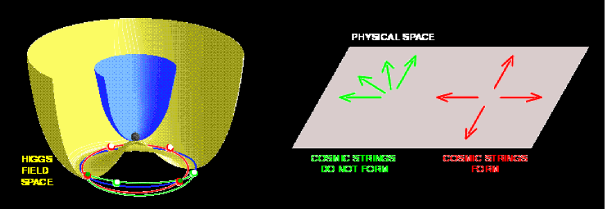
Figure 3: The complex scalar Higgs field evolves in a temperature-dependent potential $V(\phi)$. At high temperatures (violet narrow surface) the vacuum expectation value of the field lies at the bottom of $V$. For lower temperatures, the potential adopts the “Mexican hat” form (yellow surface) and the field spontaneously chooses one amongst the new available (degenerate) lowest energy states (the violet circle along the valley of the hat). This isolates a single value/direction for the phase of the field, spontaneously breaking the symmetry possessed by the system at high energies. Different regions of the universe, with no causal connection, will end up having arbitrarily different directions for the field (arrows on the right). As separate regions of broken symmetry merge, it is not always possible for the field orientations to match. It may happen that a closed loop in physical space intersects regions where the Higgs phase varies from 0 to 2$\pi$ (red arrows, corresponding to the red dashed-line on the left panel). In that situation, a cosmic string will pass somewhere inside the loop. On the contrary, green arrows (and green dashed-line on the left panel) show a situation where no string is formed after the phase transition.

Now, as we have seen earlier, due to the overall cooling down of the universe, there will be regions where the scalar field rolls down to different vacuum states. The choice of the vacuum is totally independent for regions separated apart by one correlation length or more, thus leading to the formation of domains of size $\xi\sim\eta^{-1}$. When these domains coalesce they give rise to edges in the interface. If we now draw a imaginary circle around one of these edges and the angle $\theta$ varies by $2\pi$ then by contracting this loop we reach a point where we cannot go any further without leaving the manifold ${\cal M}$. This is a small region where the variable $\theta$ is not defined and, by continuity, the field should be $\phi=0$. In order to minimize the spatial gradient energy these small regions line up and form a line–like defect called cosmic string.

The width of the string is roughly $m_{\phi}^{-1}\sim(\sqrt{\lambda}\eta)^{-1}$, $m_{\phi}$ being the Higgs mass. The string mass per unit length, or tension, is $\mu\sim\eta^{2}$. This means that for GUT cosmic strings, where $\eta\sim 10^{16}$ GeV, we have $G\mu\sim 10^{-6}$. We will see below that the dimensionless combination $G\mu$, present in all signatures due to strings, is of the right order of magnitude for rendering these defects cosmologically interesting.

There is an important difference between global and gauge (or local) cosmic strings: local strings have their energy confined mainly in a thin core, due to the presence of gauge fields $A_{\mu}$ that cancel the gradients of the field outside of it. Also these gauge fields make it possible for the string to have a quantized magnetic flux along the core. On the other hand, if the string was generated from the breakdown of a global symmetry there are no gauge fields, just Goldstone bosons, which, being massless, give rise to long–range forces. No gauge fields can compensate the gradients of $\phi$ this time and therefore there is an infinite string mass per unit length.

Just to get a rough idea of the kind of models studied in the literature, consider the case ${\bf G}=SO(10)$ that is broken to ${\bf H}=SU(5)\times{\cal Z}_{2}$. For this pattern we have $\pi_{1}({\cal M})={\cal Z}_{2}$, which is clearly non trivial and therefore cosmic strings are formed [Kibble et al., 1982].

II.4 String loops and scaling

We saw before the reasons why gauge monopoles and domain walls were a bit of a problem for cosmology. Essentially, the problem was that their energy density decreases more slowly than the critical density with the expansion of the universe. This fact resulted in their contribution to $\Omega_{\rm def}$ (the density in defects normalized by the critical density) being largely in excess compared to 1, hence in blatant conflict with modern observations. The question now arises as to whether the same might happened with cosmic strings. Are strings dominating the energy density of the universe? Fortunately, the answer to this question is no; strings evolve in such a way to make their density $\rho_{\rm strings}\propto\eta^{2}t^{-2}$. Hence, one gets the same temporal behavior as for the critical density. The result is that $\Omega_{\rm strings}\sim G\mu\sim(\eta/m_{P})^{2}\sim 10^{-6}$ for GUT strings, i.e., we get an interestingly small enough, constant fraction of the critical density of the universe and strings never upset standard observational cosmology.

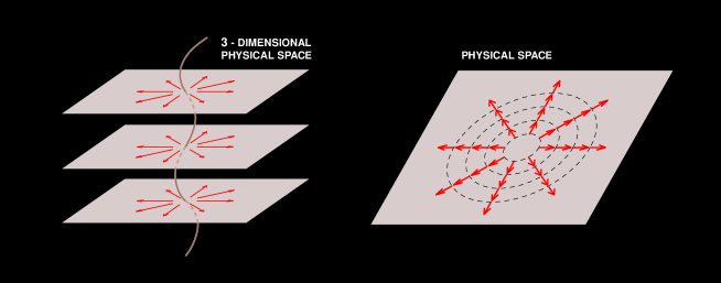
Figure 4: We can now extend the mechanism shown in the previous figure to the full three-dimensional space. Regions of the various planes that were traversed by strings can be superposed to show the actual location of the cosmic string (left panel). The figure on the right panel shows why we are sure a string crosses the plane inside the loop in physical space (the case with red arrows in the previous figure). Continuity of the field imposes that if we gradually contract this loop the direction of the field will be forced to wind “faster”. In the limit in which the loop reduces to a point, the phase is no longer defined and the vacuum expectation value of the Higgs field has to vanish. This corresponds to the central tip of the Mexican hat potential in the previous figure and is precisely the locus of the false vacuum. Cosmic strings are just that, narrow, extremely massive line-like regions in physical space where the Higgs field adopts its high-energy false vacuum state.

Now, why this is so? The answer is simply the efficient way in which a network of strings looses energy. The evolution of the string network is highly nontrivial and loops are continuously chopped off from the main infinite strings as the result of (self) intersections within the infinite–string network. Once they are produced, loops oscillate due to their huge tension and slowly decay by emitting gravitational radiation. Thus, energy is transferred from the cosmic string network to radiation.

It turns out from simulations that most of the energy in the string network (roughly a 80%) is in the form of infinite strings. Soon after formation one would expect long strings to have the form of random-walk with characteristic step given by the correlation length $\xi$. Also, the typical distance between long string segments should also be of order $\xi$. Monte Carlo simulations show that these strings are Brownian on sufficiently large scales, which means that the length $\ell$ of a string is related to the end-to-end distance ${\rm d}$ of two given points along the string (with ${\rm d}\gg\xi$) in the form

$$\ell={\rm d}^{2}/\xi.$$ (7)

What remains of the energy is given in the form of closed loops with no preferred length scale (a scale invariant distribution) which implies that the number density of loops having sizes between $R$ and $R+dR$ follows just from dimensional analysis

$$dn_{\rm loops}\propto{dR\over R^{4}}$$ (8)

which is just another way of saying that $n_{\rm loops}\propto 1/R^{3}$, loops behave like normal nonrelativistic matter. The actual coefficient, as usual, comes from string simulations.

There are both analytical and numerical indications in favor of the existence of a stable “scaling solution” for the cosmic string network. After generation, the network quickly evolves in a self similar manner with just a few infinite string segments per Hubble volume and Hubble time. A heuristic argument for the scaling solution due to Vilenkin [1985] is as follows.

If we take $\nu(t)$ to be the mean number of infinite string segments per Hubble volume, then the energy density in infinite strings $\rho_{\rm strings}=\rho_{\rm s}$ is

$$\rho_{\rm s}(t)=\nu(t)\eta^{2}t^{-2}=\nu(t)\mu t^{-2}.$$ (9)

Now, $\nu$ strings will typically have $\nu$ intersections, and so the number of loops $n_{\rm loops}(t)=n_{\rm l}(t)$ produced per unit volume will be proportional to $\nu^{2}$. We find

$$dn_{\rm l}\sim\nu^{2}R^{-4}dR.$$ (10)

Hence, recalling now that the loop sizes grow with the expansion like $R\propto t$ we have

$${dn_{\rm l}(t)\over dt}\sim p\nu^{2}t^{-4}$$ (11)

where $p$ is the probability of loop formation per intersection, a quantity related to the intercommuting probability, both roughly of order 1. We are now in a position to write an energy conservation equation for strings plus loops in the expanding universe. Here it is

$${d\rho_{\rm s}\over dt}+{3\over 2t}\,\rho_{\rm s}\sim-m_{\rm l}{dn_{\rm l}\over dt}\sim-\mu t{dn_{\rm l}\over dt}$$ (12)

where $m_{\rm l}=\mu t$ is just the loop mass and where the second on the left hand side is the dilution term $3H\rho_{\rm s}$ for an expanding radiation–dominated universe. The term on the right hand side amounts to the loss of energy from the long string network by the generation of small closed loops. Plugging Eqs. (9) and (11) into (12) Vilenkin finds the following kinetic equation for $\nu(t)$

$${d\nu\over dt}-\,{\nu\over{2t}}\sim-p{\nu^{2}\over t}$$ (13)

with $p\sim 1$. Thus if $\nu\gg 1$ then ${d\nu/dt}<0$ and $\nu$ tends to decrease in time, while if $\nu\ll 1$ then ${d\nu/dt}>0$ and $\nu$ increases. Hence, there will be a stable solution with $\nu\sim{\rm a~{}few}$.

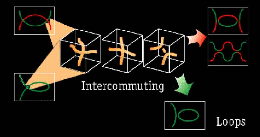
Figure 5: Global string interactions leading to loop formation. Whenever two string segments intersect, they reconnect or intercommute (green and red strings – upper part of the figure). Analogously, if a string intersects itself, it can break off a closed loop (green string – bottom part of the figure). In both cases, the interacting string segments first suffer a slight deformation (due to the long–range forces present for global strings), they subsequently fuse and finally exchange partners. A ephemeral unstable amount of energy in the form of a small loop remains in the middle where the energy is high enough to place the Higgs field in the false vacuum. It then quickly collapses, radiating away its energy. The situation is roughly the same for local strings, as simulations have shown.

II.5 Global textures

Whenever a global non–Abelian symmetry is spontaneously and completely broken (e.g. at a grand unification scale), global defects called textures are generated. Theories where this global symmetry is only partially broken do not lead to global textures, but instead to global monopoles and non–topological textures. As we already mentioned global monopoles do not suffer the same constraints as their gauge counterparts: essentially, having no associated gauge fields, the long–range forces between pairs of monopoles lead to the annihilation of their eventual excess and as a result monopoles scale with the expansion. On the other hand, non–topological textures are a generalization that allows the broken subgroup H to contain non–Abelian factors. It is then possible to have $\pi_{3}$ trivial as in, e.g., SO(5)$\to$SO(4) broken by a vector, for which case we have ${\cal M}=S^{4}$, the four–sphere [Turok, 1989]. Having explained this, let us concentrate in global topological textures from now on.

Textures, unlike monopoles or cosmic strings, are not well localized in space. This is due to the fact that the field remains in the vacuum everywhere, in contrast to what happens for other defects, where the field leaves the vacuum manifold precisely where the defect core is. Since textures do not possess a core, all the energy of the field configuration is in the form of field gradients. This fact is what makes them interesting objects only when coming from global theories: the presence of gauge fields $A_{\mu}$ could (by a suitable reorientation) compensate the gradients of $\phi$ and yield $D_{\mu}\phi=0$, hence canceling out (gauging away) the energy of the configuration.

One feature endowed by textures that really makes these defects peculiar is their being unstable to collapse. The initial field configuration is set at the phase transition, when $\phi$ develops a nonzero vacuum expectation value. $\phi$ lives in the vacuum manifold ${\cal M}$ and winds around ${\cal M}$ in a non–trivial way on scales greater than the correlation length, $\xi\hbox{ \raise 1.50696pt\hbox to0.0pt{$<$\hss}\lower 2.58334pt\hbox{$\sim$}\ }t$. The evolution is determined by the nonlinear dynamics of $\phi$. When the typical size of the defect becomes of the order of the horizon, it collapses on itself. The collapse continues until eventually the size of the defect becomes of the order of $\eta^{-1}$, and at that point the energy in gradients is large enough to raise the field from its vacuum state. This makes the defect unwind, leaving behind a trivial field configuration. As a result $\xi$ grows to about the horizon scale, and then keeps growing with it. As still larger scales come across the horizon, knots are constantly formed, since the field $\phi$ points in different directions on ${\cal M}$ in different Hubble volumes. This is the scaling regime for textures, and when it holds simulations show that one should expect to find of order 0.04 unwinding collapses per horizon volume per Hubble time [Turok, 1989]. However, unwinding events are not the most frequent feature [Borrill et al., 1994], and when one considers random field configurations without an unwinding event the number raises to about 1 collapse per horizon volume per Hubble time.

II.6 Evolution of global textures

We mentioned earlier that the breakdown of any non–Abelian global symmetry led to the formation of textures. The simplest possible example involves the breakdown of a global SU(2) by a complex doublet $\phi^{a}$, where the latter may be expressed as a four–component scalar field, i.e., $a=1\ldots 4$. We may write the Lagrangian of the theory much in the same way as it was done in Eq. (6), but now we drop the gauge fields (thus the covariant derivatives become partial derivatives). Let us take the symmetry breaking potential as follows, $V(\phi)={\lambda\over 4}\left(|\phi|^{2}-{\eta}^{2}\right)^{2}$. The situation in which a global SU(2) in broken by a complex doublet with this potential $V$ is equivalent to the theory where SO(4) is broken by a four–component vector to SO(3), by making $\phi^{a}$ take on a vacuum expectation value. We then have the vacuum manifold ${\cal M}$ given by SO(4)/SO(3) = $S^{3}$, namely, a three–sphere with $\phi^{a}\phi_{a}=\eta^{2}$. As $\pi_{3}(S^{3})\not={\bf 1}$ (in fact, $\pi_{3}(S^{3})={\cal Z}$) we see we will have non–trivial solutions of the field $\phi^{a}$ and global textures will arise.

As usual, variation of the action with respect to the field $\phi^{a}$ yields the equation of motion

$${\phi^{b}}^{\prime\prime}+2{a^{\prime}\over a}{\phi^{b}}^{\prime}-\nabla^{2}\phi^{b}=-a^{2}{\partial V\over\partial\phi^{b}}~{},$$ (14)

where primes denote derivatives with respect to conformal time and $\nabla$ is computed in comoving coordinates. When the symmetry in broken three of the initially four degrees of freedom go into massless Goldstone bosons associated with the three directions tangential to the vacuum three–sphere. The ‘radial’ massive mode that remains ($m_{\phi}\sim\sqrt{\lambda}\eta$) will not be excited, provided we concentrate on length scales much larger than $m_{\phi}^{-1}$.

To solve for the dynamics of the field $\phi^{b}$, two different approaches have been implemented in the literature. The first one faces directly the full equation (14), trying to solve it numerically. The alternative to this exploits the fact that, at temperatures smaller than $T_{c}$, the field is constrained to live in the true vacuum. By implementing this fact via a Lagrange multiplier we get

$$\nabla^{\mu}\nabla_{\mu}\phi^{b}=-{\nabla^{\mu}\phi^{c}\nabla_{\mu}\phi_{c}\over\eta^{2}}\phi^{b}~{}~{};~{}~{}\phi^{2}=\eta^{2}~{},$$ (15)

with $\nabla^{\mu}$ the covariant derivative operator. Eq. (15) represents a non–linear sigma model for the interaction of the three massless modes [Rajaraman, 1982]. This last approach is only valid when probing length scales larger than the inverse of the mass $m_{\phi}^{-1}$. As we mentioned before, when this condition is not met the gradients of the field are strong enough to make it leave the vacuum manifold and unwind.

The approach (cf. Eqs. (15)) is suitable for analytic inspection. In fact, an exact flat space solution was found assuming a spherically symmetric ansatz. This solution represents the collapse and subsequent conversion of a texture knot into massless Goldstone bosons, and is known as the spherically symmetric self–similar (SSSS) exact unwinding solution. We will say no more here with regard to the this solution, but just refer the interested reader to the original articles [see, e.g., Turok & Spergel, 1990; Notzold, 1991]. Simulations taking full account of the energy stored in gradients of the field, and not just in the unwinding events, like in Eq. (14), were performed, for example, in [Durrer & Zhou, 1995].

III Currents along strings

In the past few years it has become clear that topological defects, and in particular strings, will be endowed with a considerably richer structure than previously envisaged. In generic grand unified models the Higgs field, responsible for the existence of cosmic strings, will have interactions with other fundamental fields. This should not surprise us, for well understood low energy particle theories include field interactions in order to account for the well measured masses of light fermions, like the familiar electron, and for the masses of gauge bosons $W$ and $Z$ discovered at CERN in the eighties. Thus, when one of these fundamental (electromagnetically charged) fields present in the model condenses in the interior space of the string, there will appear electric currents flowing along the string core.

Even though these strings are the most attractive ones, the fact of them having electromagnetic properties is not actually fundamental for understanding the dynamics of circular string loops. In fact, while in the uncharged and non current-carrying case symmetry arguments do not allow us to distinguish the existence of rigid rotations around the loop axis, the very existence of a small current breaks this symmetry, marking a definite direction, which allows the whole loop configuration to rotate. This can also be viewed as the existence of spinning particle–like solutions trapped inside the core. The stationary loop solutions where the string tension gets balanced by the angular momentum of the charges is what Davis and Shellard [1988] dubbed vortons.

Vorton configurations do not radiate classically. Because they have loop shapes, implying periodic boundary conditions on the charged fields, it is not surprising that these configurations are quantized. At large distances these vortons look like point masses with quantized electric charge (actually they can have more than a hundred times the electron charge) and angular momentum. They are very much like particles, hence their name. They are however very peculiar, for their characteristic size is of order of their charge number (around a hundred) times their thickness, which is essentially some fourteen orders of magnitude smaller than the classical electron radius. Also, their mass is often of the order of the energies of grand unification, and hence vortons would be some twenty orders of magnitude heavier than the electron.

But why should strings become conducting in the first place? The physics inside the core of the string differs somewhat from outside of it. In particular the existence of interactions among the Higgs field forming the string and other fundamental fields, like that of charged fermions, would make the latter loose their masses inside the core. Then, only small energies would be required to produce pairs of trapped fermions and, being effectively massless inside the string core, they would propagate at the speed of light. These zero energy fermionic states, also called zero modes, endow the string with currents and in the case of closed loops they provide the mechanical angular momentum support necessary for stabilizing the contracting loop against collapse.

III.1 Goto–Nambu Strings

Our aim now would be to introduce extra fields into the problem and see what new features arise. We would expect to find –among other novelties– currents flowing along the defect cores, as advertised before. However, doing this in detail would unfortunately take us too much away from the main topic of these notes, and we just refer the reader to some recent work [Lemperière & Shellard 2002] (see also  CPG ; AgPpCb ) and to the recent review in boli01 , as well as to the other references given in the introduction, for a detailed treatment. Here below, we just give some few additional features of cosmic string field theory.

The simple Lagrangian we saw in previous sections was a good approximation for ideal structureless strings, known under the name of Goto–Nambu strings [Goto, 1971; Nambu, 1970]. Additional fields coupled with the string–forming Higgs field often lead to interesting effects in the form of generalized currents flowing along the string core. But before taking into full consideration the internal structure of strings (given in boli01 ) it is appropriate to start by setting the scene with the simple Abelian Higgs model (which describes scalar electrodynamics). This is a prototype of gauge field theory with spontaneous symmetry breaking G = U(1) $\to$ {1}. The Lagrangian reads [Higgs, 1964]

$${\cal L}_{{}_{\rm H}}=-{1\over 2}[{D}^{\mu}\Phi][{D}_{\mu}\Phi]^{*}-{1\over 4}(F^{(\phi)}_{\mu\nu})^{2}-{\lambda_{\phi}\over 8}(|\Phi|^{2}-\eta^{2})^{2},$$ (16)

with gauge covariant derivative $D_{\mu}=\partial_{\mu}+iqA^{(\phi)}_{\mu}$, antisymmetric tensor $F^{(\phi)}_{\mu\nu}=\nabla_{\mu}A^{(\phi)}_{\nu}-\nabla_{\nu}A^{(\phi)}_{\mu}$ for the gauge vector field $A^{(\phi)}_{\nu}$, and complex scalar field $\Phi=|\Phi|e^{i\alpha}$ with gauge coupling $q$.

The first solutions for this theory were found by Nielsen & Olesen [1973]. A couple of relevant properties are noteworthy:

• the mass per unit length for the string is $\mu=U\sim\eta^{2}$. For GUT local strings this gives $\mu\sim 10^{22}{\rm g}/{\rm cm}$, while one finds $\mu\sim\eta^{2}\ln(r/m_{\rm s}^{-1})\to\infty$ if strings are global, due to the absence of compensating gauge fields. This divergence is in general not an issue, because global strings only in few instances are isolated; in a string network, a natural cutoff is the distance to the neighboring string.

• There are essentially two characteristic mass scales (or inverse length scales) in the problem: $m_{\rm s}\sim\lambda_{\phi}^{1/2}\eta$ and $m_{\rm v}\sim q\eta$, corresponding to the inverse of the Compton wavelengths of the scalar (Higgs) and vector ($A^{(\phi)}_{\nu}$) particles, respectively.

• There exists a sort of screening of the energy, called ‘Higgs screening’, implying a finite energy configuration, thanks to the way in which the vector field behaves far from the string core: $A_{\theta}\to(1/qr)d\alpha/d\theta\,\,,{\rm~{}for~{}}r\to\infty$.

  After a closed path around the vortex one has $\Phi(2\pi)=\Phi(0)$, which implies that the winding phase $\alpha$ should be an integer times the cylindrical angle $\theta$, namely $\alpha=n\theta$. This integer $n$ is dubbed the ‘winding number’. In turn, from this fact it follows that there exists a tube of quantized ‘magnetic’ flux, given by

  $$\Phi_{{}_{\rm B}}=\oint\vec{A}.\vec{d\ell}={1\over q}\int_{0}^{2\pi}{d\alpha\over d\theta}d\theta={2\pi n\over q}$$ (17)

In the string there is a sort of competing effect between the fields: the gauge field acts in a repulsive manner; the flux doesn’t like to be confined to the core and $B$ lines repel each other. On the other hand, the scalar field behaves in an attractive way; it tries to minimize the area where $V(\Phi)\not=0$, that is, where the field departs from the true vacuum.

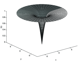
Figure 6: Higgs field and energy profiles for Goto–Nambu cosmic strings. The left panel shows the amplitude of the Higgs field around the string. The field vanishes at the origin (the false vacuum) and attains its asymptotic value (normalized to unity in the figure) far away from the origin. The phase of the scalar field (changing from 0 to $2\pi$) is shown by the shading of the surface. In the right panel we show the energy density of the configuration. The maximum value is reached at the origin, exactly where the Higgs is placed in the false vacuum. [Hindmarsh & Kibble, 1995].

Finally, we can mention a few condensed–matter ‘cousins’ of Goto–Nambu strings: flux tubes in superconductors [Abrikosov, 1957] for the nonrelativistic version of gauge strings ($\Phi$ corresponds to the Cooper pair wave function). Also, vortices in superfluids, for the nonrelativistic version of global strings ($\Phi$ corresponds to the Bose condensate wave function). Moreover, the only two relevant scales of the problem we mentioned above are the Higgs mass $m_{\rm s}$ and the gauge vector mass $m_{\rm v}$. Their inverse give an idea of the characteristic scales on which the fields acquire their asymptotic solutions far away from the string ‘location’. In fact, the relevant core widths of the string are given by $m_{\rm s}^{-1}$ and $m_{\rm v}^{-1}$. It is the comparison of these scales that draws the dividing line between two qualitatively different types of solutions. If we define the parameter $\beta=({m_{\rm s}/m_{\rm v}})^{2}$, superconductivity theory says that $\beta<1$ corresponds to Type I behavior while $\beta>1$ corresponds to Type II. For us, $\beta<1$ implies that the characteristic scale for the vector field is smaller than that for the Higgs field and so magnetic field $B$ flux lines are well confined in the core; eventually, an $n$–vortex string with high winding number $n$ stays stable. On the contrary, $\beta>1$ says that the characteristic scale for the vector field exceeds that for the scalar field and thus $B$ flux lines are not confined; the $n$–vortex string will eventually split into $n$ vortices of flux $2\pi/q$. In summary:

$$\beta=({m_{\rm s}\over m_{\rm v}})^{2}\cases{<1{\it~{}n\!\!-\!\!vortex~{}stable~{}(B~{}flux~{}lines~{}confined~{}in~{}core){\rm~{}~{}-Type~{}I}}\cr>1{\it~{}Unstable:~{}splitting~{}into~{}n~{}vortices~{}of~{}flux~{}}2\pi/q{\rm~{}-Type~{}II}}$$ (18)

IV Structure formation from defects

IV.1 Cosmic strings

In this section we will provide just a quick description of the remarkable cosmological features of cosmic strings. Many of the proposed observational tests for the existence of cosmic strings are based on their gravitational interactions. In fact, the gravitational field around a straight static string is very unusual [Vilenkin, 1981]. As is well known, the Newtonian limit of Einstein field equations with source term given by $T^{\mu}_{\nu}={\rm diag}(\rho,-p_{1},-p_{2},-p_{3})$ in terms of the Newtonian potential $\Phi$ is given by $\nabla^{2}\Phi=4\pi G(\rho+p_{1}+p_{2}+p_{3})$, just a statement of the well known fact that pressure terms also contribute to the ‘gravitational mass’. For an infinite string in the $z$–direction one has $p_{3}=-\rho$, i.e., strings possess a large relativistic tension (negative pressure). Moreover, averaging on the string core results in vanishing pressures for the $x$ and $y$ directions yielding $\nabla^{2}\Phi=0$ for the Poisson equation. This indicates that space is flat outside of an infinite straight cosmic string and therefore test particles in its vicinity should not feel any gravitational attraction.

In fact, a full general relativistic analysis confirms this and test particles in the space around the string feel no Newtonian attraction; however there exists something unusual, a sort of wedge missing from the space surrounding the string and called the ‘deficit angle’, usually noted $\Delta$, that makes the topology of space around the string that of a cone. To see this, consider the metric of a source with energy–momentum tensor [Vilenkin 1981, Gott 1985]

$$T_{\mu}^{\nu}=\delta(x)\delta(y){\rm diag}(\mu,0,0,T)\ .$$ (19)

In the case with $T=\mu$ (a rather simple equation of state) this is the effective energy–momentum tensor of an unperturbed string with string tension $\mu$ as seen from distances much larger than the thickness of the string (a Goto–Nambu string). However, real strings develop small–scale structure and are therefore not well described by the Goto–Nambu action. When perturbations are taken into account $T$ and $\mu$ are no longer equal and can only be interpreted as effective quantities for an observer who cannot resolve the perturbations along its length. And in this case we are left without an effective equation of state. Carter [1990] has proposed that these ‘noisy’ strings should be such that both its speeds of propagation of perturbations coincide. Namely, the transverse (wiggle) speed $c_{\rm T}=(T/\mu)^{1/2}$ for extrinsic perturbations should be equal to the longitudinal (woggle) speed $c_{\rm L}=(-dT/d\mu)^{1/2}$ for sound–type perturbations. This requirement yields the new equation of state

$$\mu T=\mu_{0}^{2}$$ (20)

and, when this is satisfied, it describes the energy-momentum tensor of a wiggly string as seen by an observer who cannot resolve the wiggles or other irregularities along the string [Carter 1990, Vilenkin 1990].

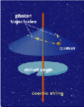
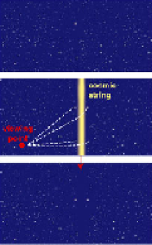
Figure 7: Cosmic strings affect surrounding spacetime by removing a small angular wedge, creating a conelike geometry (left). Space remains flat everywhere, but a circular path around the string encompasses slightly less than 360 degrees. The deficit angle is tiny, about $10^{-5}$ radian. To an observer, the presence of a cosmic string would be betrayed by its effect on the trajectory of passing light rays, which are deflected by an amount equal to the deficit angle. The resultant gravitational lensing reveals itself in the doubling of images of objects behind the string (right panel).

The gravitational field around the cosmic string [neglecting terms of order $(G\mu)^{2}$] is found by solving the linearized Einstein equations with the above $T_{\mu}^{\nu}$. One gets

$$h_{00}=h_{33}=4G(\mu-T)\ln(r/r_{0}),$$ (21)

$$h_{11}=h_{22}=4G(\mu+T)\ln(r/r_{0}),$$ (22)

where $h_{\mu\nu}=g_{\mu\nu}-\eta_{\mu\nu}$ is the metric perturbation, the radial distance from the string is $r=(x^{2}+y^{2})^{1/2}$, and $r_{0}$ is a constant of integration.

For an ideal, straight, unperturbed string, the tension and mass per unit length are $T=\mu=\mu_{0}$ and one gets

$$h_{00}=h_{33}=0,\ \ \ h_{11}=h_{22}=8G\mu_{0}\ln(r/r_{0}).$$ (23)

By a coordinate transformation one can bring this metric to a locally flat form

$$ds^{2}=dt^{2}-dz^{2}-dr^{2}-(1-8G\mu_{0})r^{2}d\phi^{2},$$ (24)

which describes a conical and flat (Euclidean) space with a wedge of angular size $\Delta=8\pi G\mu_{0}$ (the deficit angle) removed from the plane and with the two faces of the wedge identified.

IV.1.1 Wakes and gravitational lensing

We saw above that test particles at rest in the spacetime of the straight string experience no gravitational force, but if the string moves the situation radically changes. Two particles initially at rest while the string is far away, will suddenly begin moving towards each other after the string has passed between them. Their head–on velocities will be proportional to $\Delta$ or, more precisely, the particles will get a boost $v=4\pi G\mu_{0}v_{s}\gamma$ in the direction of the surface swept out by the string. Here, $\gamma=(1-v_{s}^{2})^{-1/2}$ is the Lorentz factor and $v_{s}$ the velocity of the moving string. Hence, the moving string will built up a wake of particles behind it that may eventually form the ‘seed’ for accreting more matter into sheet–like structures [Silk & Vilenkin 1984].

Figure 8: By deflecting the trajectory of ordinary matter, strings offer an interesting means of forming large-scale structure. A string sweeping through a distribution of interstellar dust will draw particles together in its wake, giving them lateral velocities of a few kilometers per second. The trail of the moving string will become a planar region of high-density matter, which, after gravitational collapse, could turn into thin, sheetlike distributions of galaxies [Image courtesy of Pedro Avelino and Paul Shellard].

Also, the peculiar topology around the string makes it act as a cylindric gravitational lens that may produce double images of distant light sources, e.g., quasars. The angle between the two images produced by a typical GUT string would be $\propto G\mu$ and of order of a few arcseconds, independent of the impact parameter and with no relative magnification between the images [see Cowie & Hu, 1987, for a first observational attempt]. Surprisingly enough, a recent detection of an extragalactic double source with the appropriate characteristics (few arcseconds angle, lack of excess light in between the images, etc), lead Sazhin et al. [2003] to propose the serendipitous discovery of a cosmic string lens event. Their data suggest that both images belong to early-type giant elliptical galaxies with redshift 0.46 (or some 1900 Mpc away, for a reduced Hubble constant $h=0.65$) meaning that these galaxies (if indeed there is such chance projection) are some 20 Kpc away from each other. On the contrary, if this pair is caused by the splitting due to an intervening cosmic string, the energy-scale of the symmetry-breaking transition giving bith to such string can be computed, and it turns out to be of a typical GUT scale. Doubtless, more independent observations are needed to confirm this interesting case.

Turning back now to the peculiar matter structures generated by moving strings, the situation described above gets even more interesting when we allow the string to have small–scale structure, which we called wiggles, as in fact simulations indicate. Wiggles not only modify the string’s effective mass per unit length, $\mu$, but also built up a Newtonian attractive term in the velocity boost inflicted on nearby test particles. To see this, let us consider the formation of a wake behind a moving wiggly string. Assuming the string moves along the $x$–axis, we can describe the situation in the rest frame of the string. In this frame, it is the particles that move, and these flow past the string with a velocity $v_{s}$ in the opposite direction. Using conformally Minkowskian coordinates we can express the relevant components of the metric as

$$ds^{2}=(1+h_{00})[dt^{2}-(dx^{2}+dy^{2})],$$ (25)

where the missing wedge is reproduced by identifying the half-lines $y=\pm 4\pi G\mu x$, $x\geq 0$. The linearized geodesic equations in this metric can be written as

$$2\ddot{x}=-(1-{\dot{x}}^{2}-{\dot{y}}^{2})\partial_{x}h_{00},$$ (26)

$$2\ddot{y}=-(1-{\dot{x}}^{2}-{\dot{y}}^{2})\partial_{y}h_{00},$$ (27)

where over–dots denote derivatives with respect to $t$. Working to first order in $G\mu$, the second of these equations can be integrated over the unperturbed trajectory $x=v_{s}t$, $y=y_{0}$. Transforming back to the frame in which the string has a velocity $v_{s}$ yields the result for the velocity impulse in the $y$–direction after the string has passed [Vachaspati & Vilenkin, 1991; Vollick, 1992]

$$v=-{{2\pi G(\mu-T)}\over{v_{s}\gamma}}-4\pi G\mu v_{s}\gamma$$ (28)

The second term is the velocity impulse due to the conical deficit angle we saw above. This term will dominate for large string velocities, case in which big planar wakes are predicted. In this case, the string wiggles will produce inhomogeneities in the wake and may easy the fragmentation of the structure. The ‘top–down’ scenario of structure formation thus follows naturally in a universe with fast-moving strings. On the contrary, for small velocities, it is the first term that dominates over the deflection of particles. The origin of this term can be easily understood [Vilenkin & Shellard, 2000]. From Eqn. (21), the gravitational force on a non–relativistic particle of mass $m$ is $F\sim mG(\mu-T)/r$. A particle with an impact parameter $r$ is exposed to this force for a time $\Delta t\sim r/v_{s}$ and the resulting velocity is $v\sim(F/m)\Delta t\sim G(\mu-T)/v_{s}$.

IV.2 Textures

During the radiation era, and when the correlation length is already growing with the Hubble radius, the texture field has energy density $\rho_{texture}\sim(\nabla\phi)^{2}\sim\eta^{2}/H^{-2}$, and remains a fixed fraction of the total density $\rho_{c}\sim t^{-2}$ yielding $\Omega_{texture}\sim G\eta^{2}$. This is the scaling behavior for textures and thus we do not need to worry about textures dominating the universe.

But as we already mentioned, textures are unstable to collapse, and this collapse generates perturbations in the metric of spacetime that eventually lead to large scale structure formation. These perturbations in turn will affect the photon geodesics leading to CMB anisotropies, the clearest possible signature to probe the existence of these exotic objects being the appearance of hot and cold spots in the microwave maps. Due to their scaling behavior, the density fluctuations induced by textures on any scale at horizon crossing are given by $(\delta\rho/\rho)_{H}\sim G\eta^{2}$. CMB temperature anisotropies will be of the same amplitude. Numerically–simulated maps, with patterns smoothed over $10^{\circ}$ angular scales, by Bennett & Rhie [1993] yield, upon normalization to the COBE–DMR data, a dimensionless value $G\eta^{2}\sim 10^{-6}$, in good agreement with a GUT phase transition energy scale. It is fair to say, however, that the texture scenario is having problems in matching current data on smaller scales [see, e.g., Durrer, 2000].

IV.3 Defects as dark energy

There is recent mounting evidence that our current universe is being dominated by a unexpectedly large amount of dark energy [e.g., Riess et al., 1998; Perlmutter et al., 1999]. Recent observations with type Ia supernovae, together with other astrophysical tests, suggest that more than 65 percent of the critical energy density is made up by some yet unknown energy component.

Cosmic defects can also be seen as a novel form of dark energy. For example, a tangled web of cosmic strings with fixed mass per unit length, which self–intersects without having reconnection. Non intercommuting strings means no production of loops, and therefore the main channel for loosing energy is not active. The model proposed in [Vilenkin, 1984] has the mean mass density in strings scaling as $\rho_{\rm strings}\propto(ta(t))^{-1}$ instead of $\rho_{\rm strings}\propto\eta^{2}t^{-2}$ as we saw above. From this, one has $\rho_{\rm strings}t^{2}\propto t^{1/2}$ in the radiation–dominated era and $\rho_{\rm strings}t^{2}\propto t^{1/3}$ during matter domination, which means that the energy in strings $\Omega_{\rm strings}$ grows with time and, after a certain $t_{s}$, strings would dominate the universe. With $t_{s}$ falling in the matter–domination era, we have $\rho_{\rm strings}/\rho(t_{s})\sim(t_{\rm eq}/t_{*})^{1/2}(t_{s}/t_{\rm eq})^{1/3}G\mu\sim 1$, with the background $\rho\propto 1/Gt^{2}$. In the case $0<z\hbox{ \raise 1.50696pt\hbox to0.0pt{$<$\hss}\lower 2.58334pt\hbox{$\sim$}\ }3$, roughly $t_{s}\sim 10^{17}$ sec., with $t_{\rm eq}\sim 10^{11}$ sec. and $t_{*}\sim m_{P}/\eta^{2}$, we get $G\mu\sim 10^{-20}$ for the characteristic energy scale of these non–intercommuting strings.

After $t_{s}$ the Friedmann’s equation can be cast as $(\dot{a}/a)^{2}\propto G\rho_{\rm strings}\propto G/ta(t)$, which implies that the scale factor goes as $a(t)\propto t$ and then $\rho_{\rm strings}\propto 1/t^{2}$. Now, recalling the local energy conservation law $\dot{\rho}=-3(\rho+p)\dot{a}/a$, and applying it for a dark “$x$” component, $w_{x}=p_{x}/\rho_{x}$, we get $\rho_{x}\propto a^{-3(1+w_{x})}$. If this dark component is made up by strings, one then deduces that it should be $w_{x}=-1/3$. Of course, this gives $\ddot{a}=0$ for the scale factor, so it cannot explain the recent acceleration phase. It nevertheless goes in the right direction.

Similar arguments have been studied for other defects, like textures [Davis, 1987] and can also be devised for domain walls [Zel’dovich et al., 1974; Battye et al., 1999], in this latter case yielding $w_{x}=-2/3$ which points closer to the observational “equation of state” currently selected by the analysis of the different astrophysical surveys. For these and other reasons, with the words of the recent authoritative review by Peebles & Ratra [2002], the class of cosmic defect models is worth bearing in mind.

V CMB signatures from defects

If cosmic defects have really formed in the early universe and some of them are still within our present horizon today, the anisotropies in the CMB they produce would have a characteristic signature. Strings, for example, would imprint the background radiation in a very particular way due to the Doppler shift that the background radiation suffers when a string intersects the line of sight. The conical topology of space around the string will produce a differential redshift of photons passing on different sides of it, resulting in step–like discontinuities in the effective CMB temperature, given by ${\Delta T\over T}\approx 8\pi G\mu v_{s}\gamma$ with, as before, $\gamma=(1-v_{s}^{2})^{-1/2}$ the Lorentz factor and $v_{s}$ the velocity of the moving string. This ‘stringy’ signature was first studied by Kaiser & Stebbins [1984] and Gott [1985] (see Figure 9).

Figure 9: The Kaiser-Stebbins effect for cosmic strings. A string network evolves into a self-similar scaling regime, perturbing matter and radiation during its evolution. The effect on the CMB after recombination leads to distinct steplike discontinuities on small angular scales that were first studied by Kaiser & Stebbins [1984]. The left panel shows a simulated patch of the sky that fits in one of the pixels of the COBE experiment. Hence, higher resolution observatories are needed in order to detect strings. The right panel shows a patch on the CMB sky of order 20’ across. However, recent studies indicate that this clean tell-tale signal gets obscured at subdegree angular scales due to the temperature fluctuations generated before recombination. [Magueijo & Ferreira 1997].

Anisotropies of the CMB are directly related to the origin of structure in the universe. Galaxies and clusters of galaxies eventually formed by gravitational instability from primordial density fluctuations, and these same fluctuations left their imprint on the CMB. Recent balloon [de Bernardis, et al., 2000; Hanany, et al., 2000], ground-based interferometer [Halverson, et al., 2001] and satellite [Bennett, et al. 2003] experiments have produced reliable estimates of the power spectrum of the CMB temperature anisotropies. While they helped eliminate certain candidate theories for the primary source of cosmic perturbations, the power spectrum data is still compatible with the theoretical estimates of a relatively large variety of models, such as $\Lambda$CDM, quintessence models or some hybrid models including cosmic defects.

There are two main classes of models of structure formation –passive and active models. In passive models, density inhomogeneities are set as initial conditions at some early time, and while they subsequently evolve as described by Einstein–Boltzmann equations, no additional perturbations are seeded. On the other hand, in active models the sources of density perturbations are time–dependent.

All specific realizations of passive models are based on the idea of inflation. In simplest inflationary models it is assumed that there exists a weakly coupled scalar field $\phi$, called the inflaton, which “drives” the (quasi) exponential expansion of the universe. The quantum fluctuations of $\phi$ are stretched by the expansion to scales beyond the horizon, thus “freezing” their amplitude. Inflation is followed by a period of thermalization, during which standard forms of matter and energy are formed. Because of the spatial variations of $\phi$ introduced by quantum fluctuations, thermalization occurs at slightly different times in different parts of the universe. Such fluctuations in the thermalization time give rise to density fluctuations. Because of their quantum nature and because of the fact that initial perturbations are assumed to be in the vacuum state and hence well described by a Gaussian distribution, perturbations produced during inflation are expected to follow Gaussian statistics to a high degree [Gangui, Lucchin, Matarrese & Mollerach, 1994], or either be products of Gaussian random variables. This is a fairly general prediction that is being tested currently with data from WMAP and will be tested more thoroughly in the future with Planck.

Active models of structure formation are motivated by cosmic topological defects with the most promising candidates being cosmic strings. As we saw in previous sections, it is widely believed that the universe underwent a series of phase transitions as it cooled down due to the expansion. If our ideas about grand unification are correct, then some cosmic defects should have formed during phase transitions in the early universe. Once formed, cosmic strings could survive long enough to seed density perturbations. Defect models possess the attractive feature that they have no parameter freedom, as all the necessary information is in principle contained in the underlying particle physics model. Generically, perturbations produced by active models are not expected to be Gaussian distributed [Gangui, Pogosian & Winitzki, 2001a].

V.1 CMB power spectrum from strings

The narrow main peak and the presence of the second and the third peaks in the CMB angular power spectrum, as measured by BOOMERANG, MAXIMA, DASI and WMAP [de Bernardis, et al., 2000; Hanany, et al., 2000; Halverson, et al., 2001; Page, et al., 2003], is an evidence for coherent oscillations of the photon–baryon fluid at the beginning of the decoupling epoch [see, e.g., Gangui, 2001]. While such coherence is a property of all passive model, realistic cosmic string models produce highly incoherent perturbations that result in a much broader main peak. This excludes cosmic strings as the primary source of density fluctuations unless new physics is postulated, e.g. models with a varying speed of light [Avelino & Martins, 2000]. In addition to purely active or passive models, it has been recently suggested that perturbations could be seeded by some combination of the two mechanisms. For example, cosmic strings could have formed just before the end of inflation and partially contributed to seeding density fluctuations. It has been shown [Contaldi, et al., 1999; Battye & Weller, 2000; Bouchet, et al., 2001] that, although not compelling, such hybrid models can be rather successful in fitting the CMB power spectrum data.

Calculating CMB anisotropies sourced by topological defects is a rather difficult task. In inflationary scenario the entire information about the seeds is contained in the initial conditions for the perturbations in the metric. In the case of cosmic defects, perturbations are continuously seeded over the period of time from the phase transition that had produced them until today. The exact determination of the resulting anisotropy requires, in principle, the knowledge of the energy–momentum tensor [or, if only two point functions are being calculated, the unequal time correlators, Pen, Seljak, & Turok, 1997] of the defect network and the products of its decay at all times. This information is simply not available. Instead, a number of clever simplifications, based on the expected properties of the defect networks (e.g. scaling), are used to calculate the source. The latest data from BOOMERANG, MAXIMA and WMAP experiments clearly disagree with the predictions of these simple models of defects [Durrer, Gangui & Sakellariadou, 1996].

The shape of the CMB angular power spectrum is determined by three main factors: the geometry of the universe, coherence and causality. The curvature of the universe directly affects the paths of light rays coming to us from the surface of last scattering. In a closed universe, because of the lensing effect induced by the positive curvature, the same physical distances between points on the sky would correspond to larger angular scales. As a result, the peak structure in the CMB angular power spectrum would shift to larger angular scales or, equivalently, to smaller values of the multipoles $\ell$’s.

The prediction of the cosmic string model of [Pogosian & Vachaspati, 1999] for $\Omega_{\rm total}=1.3$ is shown in Figure 10. As can be seen, the main peak in the angular power spectrum can be matched by choosing a reasonable value for $\Omega_{\rm total}$. However, even with the main peak in the right place the agreement with the data is far from satisfactory. The peak is significantly wider than that in the data and there is no sign of a rise in power at multipole roughly $l\approx 400$ as the actual data from WMAP suggests. The sharpness and the height of the main peak in the angular spectrum can be enhanced by including the effects of gravitational radiation [Contaldi, Hindmarsh & Magueijo, 1999] and wiggles [Pogosian & Vachaspati, 1999]. More precise high–resolution numerical simulations of string networks in realistic cosmologies with a large contribution from $\Omega_{\Lambda}$ are needed to determine the exact amount of small–scale structure on the strings and the nature of the products of their decay [Landriau & Shellard, 2002]. It is, however, unlikely that including these effects alone would result in a sufficiently narrow main peak and some presence of a second peak.

Figure 10: The CMB power spectrum produced by the wiggly string model of [Pogosian & Vachaspati, 1999] in a closed universe with $\Omega_{\rm total}=1.3$, $\Omega_{\rm baryon}=0.05$, $\Omega_{\rm CDM}=0.35$, $\Omega_{\Lambda}=0.9$, and $H_{0}=65{\rm~{}km~{}s}^{-1}{\rm Mpc}^{-1}$ [Pogosian, 2001].

This brings us to the issues of causality and coherence and how the random nature of the string networks comes into the calculation of the anisotropy spectrum. Both experimental and theoretical results for the CMB power spectra involve calculations of averages. When estimating the correlations of the observed temperature anisotropies, it is usual to compute the average over all available patches on the sky. When calculating the predictions of their models, theorists find the average over the ensemble of possible outcomes provided by the model.

In inflationary models, as in all passive models, only the initial conditions for the perturbations are random. The subsequent evolution is the same for all members of the ensemble. For wavelengths higher than the Hubble radius, the linear evolution equations for the Fourier components of such perturbations have a growing and a decaying solution. The modes corresponding to smaller wavelengths have only oscillating solutions. As a consequence, prior to entering the horizon, each mode undergoes a period of phase “squeezing” which leaves it in a highly coherent state by the time it starts to oscillate. Coherence here means that all members of the ensemble, corresponding to the same Fourier mode, have the same temporal phase. So even though there is randomness involved, as one has to draw random amplitudes for the oscillations of a given mode, the time behavior of different members of the ensemble is highly correlated. The total spectrum is the ensemble–averaged superposition of all Fourier modes, and the predicted coherence results in an interference pattern seen in the angular power spectrum as the well–known acoustic peaks.

In contrast, the evolution of the string network is highly non-linear. Cosmic strings are expected to move at relativistic speeds, self–intersect and reconnect in a chaotic fashion. The consequence of this behavior is that the unequal time correlators of the string energy–momentum vanish for time differences larger than a certain coherence time ($\tau_{c}$ in Figure 11). Members of the ensemble corresponding to a given mode of perturbations will have random temporal phases with the “dice” thrown on average once in each coherence time. The coherence time of a realistic string network is rather short. As a result, the interference pattern in the angular power spectrum is completely washed out.

Causality manifests itself, first of all, through the initial conditions for the string sources, the perturbations in the metric and the densities of different particle species. If one assumes that the defects are formed by a causal mechanism in an otherwise smooth universe then the correct initial condition are obtained by setting the components of the stress–energy pseudo–tensor $\tau_{\mu\nu}$ to zero [Veeraraghavan & Stebbins, 1990; Pen, Spergel & Turok, 1994]. These are the same as the isocurvature initial conditions [Hu, Spergel & White, 1997]. A generic prediction of isocurvature models (assuming perfect coherence) is that the first acoustic peak is almost completely hidden. The main peak is then the second acoustic peak and in flat geometries it appears at $\ell\approx 300-400$. This is due to the fact that after entering the horizon a given Fourier mode of the source perturbation requires time to induce perturbations in the photon density. Causality also implies that no superhorizon correlations in the string energy density are allowed. The correlation length of a “realistic” string network is normally between 0.1 and 0.4 of the horizon size.

An interesting study was performed by Magueijo, Albrecht, Ferreira & Coulson [1996], where they constructed a toy model of defects with two parameters: the coherence length and the coherence time. The coherence length was taken to be the scale at which the energy density power spectrum of the strings turns from a power law decay for large values of $k$ into a white noise at low $k$. This is essentially the scale corresponding to the correlation length of the string network. The coherence time was defined in the sense described in the beginning of this section, in particular, as the time difference needed for the unequal time correlators to vanish.

Figure 11: The predictions of the toy model of Magueijo, et al. [1996] for different values of parameters $x_{c}$, the coherence length, and $\tau_{c}$, the coherence time. $x_{c}\propto\eta/\lambda_{c}(\eta)$, where $\eta$ is the conformal time and $\lambda_{c}(\eta)$ is the correlation length of the network at time $\eta$. One can obtain oscillations in the CMB power spectrum by fixing either one of the parameters and varying the other.

Their study showed (see Figure 11) that by accepting any value for one of the parameters and varying the other (within the constraints imposed by causality) one could reproduce the oscillations in the CMB power spectrum. Unfortunately for cosmic strings, at least as we know them today, they fall into the parameter range corresponding to the upper right corner in Figure 11.

In order to get a better fit to present–day observations, cosmic strings must either be more coherent or they have to be stretched over larger distances, which is another way of making them more coherent. To understand this imagine that there was just one long straight string stretching across the universe and moving with some given velocity. The evolution of this string would be linear and the induced perturbations in the photon density would be coherent. By increasing the correlation length of the string network we would move closer to this limiting case of just one long straight string and so the coherence would be enhanced.

The question of whether or not defects can produce a pattern of the CMB power spectrum similar to, and including the acoustic peaks of, that produced by the adiabatic inflationary models was repeatedly addressed in the literature [Contaldi, Hindmarsh & Magueijo 1999; Magueijo, et al. 1996; Liddle, 1995; Turok, 1996; Avelino & Martins, 2000]. In particular, it was shown [Magueijo, et al. 1996; Turok, 1996] that one can construct a causal model of active seeds which for certain values of parameters can reproduce the oscillations in the CMB spectrum. The main problem today is that current realistic models of cosmic strings fall out of the parameter range that is needed to fit the observations. At the moment, only the (non-minimal) models with either a varying speed of light or hybrid contribution of strings+inflation are the only ones involving topological defects that to some extent can match the observations. One possible way to distinguish their predictions from those of inflationary models would be by computing key non–Gaussian statistical quantities, such as the CMB bispectrum.

V.2 CMB bispectrum from active models

Different cosmological models differ in their predictions for the statistical distribution of the anisotropies beyond the power spectrum. Current WMAP data and the future Planck satellite mission will provide high-precision data allowing definite estimates of non-Gaussian signals in the CMB. It is therefore important to know precisely which are the predictions of all candidate models for the statistical quantities that will be extracted from the new data and identify their specific signatures.

Of the available non-Gaussian statistics, the CMB bispectrum, or the three-point function of Fourier components of the temperature anisotropy, has been perhaps the one best studied in the literature [Gangui & Martin, 2000a]. There are a few cases where the bispectrum may be deduced analytically from the underlying model. The bispectrum can be estimated from simulated CMB sky maps; however, computing a large number of full-sky maps resulting from defects is a much more demanding task. Recently, a precise numerical code to compute it, not using CMB maps and similar to the CMBFAST code for the power spectrum, was developed in [Gangui, Pogosian & Winitzki 2001b]. What follows below is an account of this work.

In a few words, given a suitable model, one can generate a statistical ensemble of realizations of defect matter perturbations. We used a modified Boltzmann code based on CMBFAST to compute the effect of these perturbations on the CMB and found the bispectrum estimator for a given realization of sources. We then performed statistical averaging over the ensemble of realizations to compute the expected CMB bispectrum. (The CMB power spectrum was also obtained as a byproduct.) As a first application, we then computed the expected CMB bispectrum from a model of simulated string networks first introduced by Albrecht et al. [1997] and further developed in [Pogosian & Vachaspati, 1999] and in [Gangui, Pogosian & Winitzki 2001].

We assume that, given a model of active perturbations, such as a string simulation, we can calculate the energy-momentum tensor $T_{\mu\nu}({\mathbf{x}},\tau)$ for a particular realization of the sources in a finite spatial volume $V_{0}$. Here, ${\bf x}$ is a 3-dimensional coordinate and $\tau$ is the cosmic time. Many simulations are run to obtain an ensemble of random realizations of sources with statistical properties appropriate for the given model. The spatial Fourier decomposition of $T_{\mu\nu}$ can be written as

$$T_{\mu\nu}({{\mathbf{x}}},\tau)=\sum_{{\mathbf{k}}}\Theta_{\mu\nu}({{\mathbf{k}}},\tau)e^{i{{\mathbf{k}}}{{\mathbf{x}}}}\,\,\,,$$ (29)

where ${{\mathbf{k}}}$ are discrete. If $V_{0}$ is sufficiently large we can approximate the summation by the integral

$$\sum_{{\mathbf{k}}}\Theta_{\mu\nu}({{\mathbf{k}}},\tau)e^{i{{\mathbf{k}}}{{\mathbf{x}}}}\approx\frac{V_{0}}{(2\pi)^{3}}\int d^{3}{{\mathbf{k}}}\Theta_{\mu\nu}({{\mathbf{k}}},\tau)e^{i{{\mathbf{k}}}{{\mathbf{x}}}}\,\,\,,$$ (30)

and the corresponding inverse Fourier transform will be

$$\Theta_{\mu\nu}({{\mathbf{k}}},\tau)=\frac{1}{V_{0}}\int_{V_{0}}d^{3}{{\mathbf{x}}}\,T_{\mu\nu}({{\mathbf{x}}},\tau)e^{-i{{\mathbf{k}}}{{\mathbf{x}}}}\,\,\,.$$ (31)

Of course, the final results, such as the CMB power spectrum or bispectrum, do not depend on the choice of $V_{0}$. To ensure this independence, we shall keep $V_{0}$ in all expressions where it appears below.

It is conventional to expand the temperature fluctuations over the basis of spherical harmonics,

$${\Delta T/T}({\hat{{\mathbf{n}}}})=\sum_{lm}a_{lm}Y_{lm}({\hat{{\mathbf{n}}}}),$$ (32)

where $\hat{{\mathbf{n}}}$ is a unit vector. The coefficients $a_{lm}$ can be decomposed into Fourier modes,

$$a_{lm}=\frac{V_{0}}{(2\pi)^{3}}\left(-i\right)^{l}4\pi\int d^{3}{{\mathbf{k}}}\,\Delta_{l}\left({{\mathbf{k}}}\right)Y^{*}_{lm}({\hat{{\mathbf{k}}}}).$$ (33)

Given the sources $\Theta_{\mu\nu}({{\mathbf{k}}},\tau)$, the quantities $\Delta_{l}({{\mathbf{k}}})$ are found by solving linearized Einstein-Boltzmann equations and integrating along the line of sight, using a code similar to CMBFAST [Seljak & Zaldarriaga, 1996]. This standard procedure can be written symbolically as the action of a linear operator ${\hat{B}}_{l}^{\mu\nu}(k)$ on the source energy-momentum tensor, $\Delta_{l}({{\mathbf{k}}})={\hat{B}}_{l}^{\mu\nu}(k)\Theta_{\mu\nu}({{\mathbf{k}}},\tau)$, so the third moment of $\Delta_{l}({{\mathbf{k}}})$ is linearly related to the three-point correlator of $\Theta_{\mu\nu}({{\mathbf{k}}},\tau)$. Below we consider the quantities $\Delta_{l}({{\mathbf{k}}})$, corresponding to a set of realizations of active sources, as given. The numerical procedure for computing $\Delta_{l}({{\mathbf{k}}})$ was developed in [Albrecht et al.  1997] and in [Pogosian & Vachaspati, 1999].

The third moment of $a_{lm}$, namely $\left\langle a_{l_{1}m_{1}}a_{l_{2}m_{2}}a_{l_{3}m_{3}}\right\rangle$, can be expressed as

$$\left(-i\right)^{l_{1}+l_{2}+l_{3}}\left(4\pi\right)^{3}\!\!\frac{V_{0}^{3}}{(2\pi)^{9}}\!\!\int\!\!d^{3}{{\mathbf{k}}}_{1}d^{3}{{\mathbf{k}}}_{2}d^{3}{{\mathbf{k}}}_{3}Y^{*}_{l_{1}m_{1}}\!({\hat{{\mathbf{k}}}}_{1})Y^{*}_{l_{2}m_{2}}\!({\hat{{\mathbf{k}}}}_{2})Y^{*}_{l_{3}m_{3}}\!({\hat{{\mathbf{k}}}}_{3})\left\langle\Delta_{l_{1}}\!\!\left({{\mathbf{k}}}_{1}\right)\Delta_{l_{2}}\!\!\left({{\mathbf{k}}}_{2}\right)\Delta_{l_{3}}\!\!\left({{\mathbf{k}}}_{3}\right)\right\rangle.$$ (34)

A straightforward numerical evaluation of Eq. (34) from given sources $\Delta_{l}\left({{\mathbf{k}}}\right)$ is prohibitively difficult, because it involves too many integrations of oscillating functions. However, we shall be able to reduce the computation to integrations over scalars [a similar method was employed in Komatsu & Spergel, 2001 and in Wang & Kamionkowski, 2000]. Due to homogeneity, the 3-point function vanishes unless the triangle constraint is satisfied,

$${{\mathbf{k}}}_{1}+{{\mathbf{k}}}_{2}+{{\mathbf{k}}}_{3}=0.$$ (35)

We may write

$$\left\langle\Delta_{l_{1}}\left({{\mathbf{k}}}_{1}\right)\Delta_{l_{2}}\left({{\mathbf{k}}}_{2}\right)\Delta_{l_{3}}\left({{\mathbf{k}}}_{3}\right)\right\rangle=\delta^{(3)}\left({{\mathbf{k}}}_{1}+{{\mathbf{k}}}_{2}+{{\mathbf{k}}}_{3}\right)P_{l_{1}l_{2}l_{3}}\left({{\mathbf{k}}}_{1},{{\mathbf{k}}}_{2},{{\mathbf{k}}}_{3}\right),$$ (36)

where the three-point function $P_{l_{1}l_{2}l_{3}}\left({{\mathbf{k}}}_{1},{{\mathbf{k}}}_{2},{{\mathbf{k}}}_{3}\right)$ is defined only for values of ${\mathbf{k}}_{i}$ that satisfy Eq. (35). Given the scalar values $k_{1}$, $k_{2}$, $k_{3}$, there is a unique (up to an overall rotation) triplet of directions ${\hat{{\mathbf{k}}}}_{i}$ for which the RHS of Eq. (36) does not vanish. The quantity $P_{l_{1}l_{2}l_{3}}\left({{\mathbf{k}}}_{1},{{\mathbf{k}}}_{2},{{\mathbf{k}}}_{3}\right)$ is invariant under an overall rotation of all three vectors ${{\mathbf{k}}}_{i}$ and therefore may be equivalently represented by a function of scalar values $k_{1}$, $k_{2}$, $k_{3}$, while preserving all angular information. Hence, we can rewrite Eq. (36) as

$$\left\langle\Delta_{l_{1}}\!\!\left({{\mathbf{k}}}_{1}\right)\Delta_{l_{2}}\!\!\left({{\mathbf{k}}}_{2}\right)\Delta_{l_{3}}\!\!\left({{\mathbf{k}}}_{3}\right)\right\rangle=\delta^{(3)}\left({{\mathbf{k}}}_{1}+{{\mathbf{k}}}_{2}+{{\mathbf{k}}}_{3}\right)P_{l_{1}l_{2}l_{3}}(k_{1},k_{2},k_{3}).$$ (37)

Then, using the simulation volume $V_{0}$ explicitly, we have

$$P_{l_{1}l_{2}l_{3}}\!\left(k_{1},k_{2},k_{3}\right)\!=\!\frac{(2\pi)^{3}}{V_{0}}\left\langle\Delta_{l_{1}}\!\!\left({{\mathbf{k}}}_{1}\right)\Delta_{l_{2}}\!\!\left({{\mathbf{k}}}_{2}\right)\Delta_{l_{3}}\!\!\left({{\mathbf{k}}}_{3}\right)\right\rangle.$$ (38)

Given an arbitrary direction $\hat{{\mathbf{k}}}_{1}$ and the magnitudes $k_{1}$, $k_{2}$ and $k_{3}$, the directions $\hat{{\mathbf{k}}}_{2}$ and $\hat{{\mathbf{k}}}_{3}$ are specified up to overall rotations by the triangle constraint. Therefore, both sides of Eq. (38) are functions of scalar $k_{i}$ only. The expression on the RHS of Eq. (38) is evaluated numerically by averaging over different realizations of the sources and over permissible directions $\hat{{\mathbf{k}}}_{i}$; below we shall give more details of the procedure.

Substituting Eqs. (37) and (38) into (34), Fourier transforming the Dirac delta and using the Rayleigh identity, we can perform all angular integrations analytically and obtain a compact form for the third moment,

$$\left\langle a_{l_{1}m_{1}}a_{l_{2}m_{2}}a_{l_{3}m_{3}}\right\rangle={\mathcal{H}}_{l_{1}l_{2}l_{3}}^{m_{1}m_{2}m_{3}}\int r^{2}dr\,b_{l_{1}l_{2}l_{3}}(r),$$ (39)

where, denoting the Wigner $3j$-symbol by $\left({}^{\,\,l_{1}\,\;l_{2}\,\;l_{3}}_{m_{1}m_{2}m_{3}}\right)$, we have

$${\mathcal{H}}_{l_{1}l_{2}l_{3}}^{m_{1}m_{2}m_{3}}\equiv\sqrt{\frac{\left(2l_{1}+1\right)\left(2l_{2}+1\right)\left(2l_{3}+1\right)}{4\pi}}\left(\begin{array}[]{ccc}l_{1}&l_{2}&l_{3}\\ 0&0&0\end{array}\right)\left(\begin{array}[]{ccc}l_{1}&l_{2}&l_{3}\\ m_{1}&m_{2}&m_{3}\end{array}\right)\,,$$ (44)

and where we have defined the auxiliary quantities $b_{l_{1}l_{2}l_{3}}$ using spherical Bessel functions $j_{l}$,

$$b_{l_{1}l_{2}l_{3}}(r) \equiv \frac{8}{\pi^{3}}\frac{V_{0}^{3}}{(2\pi)^{3}}\int k_{1}^{2}dk_{1}\,k_{2}^{2}dk_{2}\,k_{3}^{2}dk_{3}\,$$ (45)

$$\times j_{l_{1}}(k_{1}r)j_{l_{2}}(k_{2}r)j_{l_{3}}(k_{3}r)P_{l_{1}l_{2}l_{3}}(k_{1},k_{2},k_{3}).$$

The volume factor $V_{0}^{3}$ contained in this expression is correct: as shown in the next section, each term $\Delta_{l}$ includes a factor $V_{0}^{-2/3}$, while the average quantity $P_{l_{1}l_{2}l_{3}}(k_{1},k_{2},k_{3})\propto V_{0}^{-3}$ [cf. Eq. (38)], so that the arbitrary volume $V_{0}$ of the simulation cancels.

Our proposed numerical procedure therefore consists of computing the RHS of Eq. (39) by evaluating the necessary integrals. For fixed $\left\{l_{1}l_{2}l_{3}\right\}$, computation of the quantities $b_{l_{1}l_{2}l_{3}}(r)$ is a triple integral over scalar $k_{i}$ defined by Eq. (45); it is followed by a fourth scalar integral over $r$ [Eq. (39)]. We also need to average over many realizations of sources to obtain $P_{l_{1}l_{2}l_{3}}\!\left(k_{1},k_{2},k_{3}\right)$. It was not feasible for us to precompute the values $P_{l_{1}l_{2}l_{3}}\!\left(k_{1},k_{2},k_{3}\right)$ on a grid before integration because of the large volume of data: for each set $\left\{l_{1}l_{2}l_{3}\right\}$ the grid must contain $\sim 10^{3}$ points for each $k_{i}$. Instead, we precompute $\Delta_{l}\!\!\left({{\mathbf{k}}}\right)$ from one realization of sources and evaluate the RHS of Eq. (38) on that data as an estimator of $P_{l_{1}l_{2}l_{3}}\!\left(k_{1},k_{2},k_{3}\right)$, averaging over allowed directions of $\hat{{\mathbf{k}}}_{i}$. The result is used for integration in Eq. (45).

Because of isotropy and since the allowed sets of directions $\hat{{\mathbf{k}}}_{i}$ are planar, it is enough to restrict the numerical calculation to directions $\hat{{\mathbf{k}}}_{i}$ within a fixed two-dimensional plane. This significantly reduces the amount of computations and data storage, since $\Delta_{l}\!\left({{\mathbf{k}}}\right)$ only needs to be stored on a two-dimensional grid of ${\mathbf{k}}$.

In estimating $P_{l_{1}l_{2}l_{3}}\!\left(k_{1},k_{2},k_{3}\right)$ from Eq. (38), averaging over directions of $\hat{{\mathbf{k}}}_{i}$ plays a similar role to ensemble averaging over source realizations. Therefore if the number of directions is large enough (we used 720 for cosmic strings), only a moderate number of different source realizations is needed. The main numerical difficulty is the highly oscillating nature of the function $b_{l_{1}l_{2}l_{3}}(r)$. The calculation of the bispectrum for cosmic strings presented in the next Section requires about 20 days of a single-CPU workstation time per realization.

We note that this method is specific for the bispectrum and cannot be applied to compute higher-order correlations. The reason is that higher-order correlations involve configurations of vectors ${\mathbf{k}}_{i}$ that are not described by scalar values $k_{i}$ and not restricted to a plane. For instance, a computation of a 4-point function would involve integration of highly oscillating functions over four vectors ${\mathbf{k}}_{i}$ which is computationally infeasible.

From Eq. (39) we derive the CMB angular bispectrum ${\mathcal{C}}_{l_{1}l_{2}l_{3}}$, defined as [Gangui & Martin, 2000b]

$$\bigl{\langle}a_{l_{1}m_{1}}a_{l_{2}m_{2}}a_{l_{3}m_{3}}\bigr{\rangle}=\left(\begin{array}[]{ccc}l_{1}&l_{2}&l_{3}\\ m_{1}&m_{2}&m_{3}\end{array}\right){\mathcal{C}}_{l_{1}l_{2}l_{3}}\,.$$ (48)

The presence of the 3$j$-symbol guarantees that the third moment vanishes unless $m_{1}+m_{2}+m_{3}=0$ and the $l_{i}$ indices satisfy the triangle rule $|l_{i}-l_{j}|\leq l_{k}\leq l_{i}+l_{j}$. Invariance under spatial inversions of the three-point correlation function implies the additional ‘selection rule’ $l_{1}+l_{2}+l_{3}=\mbox{even}$, in order for the third moment not to vanish. Finally, from this last relation and using standard properties of the 3$j$-symbols, it follows that the angular bispectrum ${\mathcal{C}}_{l_{1}l_{2}l_{3}}$ is left unchanged under any arbitrary permutation of the indices $l_{i}$.

In what follows we will restrict our calculations to the angular bispectrum $C_{l_{1}l_{2}l_{3}}$ in the ‘diagonal’ case, i.e. $l_{1}=l_{2}=l_{3}=l$. This is a representative case and, in fact, the one most frequently considered in the literature. Plots of the power spectrum are usually done in terms of $l(l+1)C_{l}$ which, apart from constant factors, is the contribution to the mean squared anisotropy of temperature fluctuations per unit logarithmic interval of $l$. In full analogy with this, the relevant quantity to work with in the case of the bispectrum is

$$G_{lll}=l(2l+1)^{3/2}\left(\begin{array}[]{ccc}l&l&l\\ 0&0&0\end{array}\right)C_{lll}\,.$$ (51)

For large values of the multipole index $l$, $G_{lll}\propto l^{3/2}C_{lll}$. Note also what happens with the 3$j$-symbols appearing in the definition of the coefficients ${\mathcal{H}}_{l_{1}l_{2}l_{3}}^{m_{1}m_{2}m_{3}}$: the symbol $\left({}^{\,\,l_{1}\,\;l_{2}\,\;l_{3}}_{m_{1}m_{2}m_{3}}\right)$ is absent from the definition of $C_{l_{1}l_{2}l_{3}}$, while in Eq. (51) the symbol $\left({}^{\,l\;l\;l}_{0\>0\>0}\right)$ is squared. Hence, there are no remnant oscillations due to the alternating sign of $\left({}^{\,l\;l\;l}_{0\>0\>0}\right)$.

However, even more important than the value of $C_{lll}$ itself is the relation between the bispectrum and the cosmic variance associated with it. In fact, it is their comparison that tells us about the observability ‘in principle’ of the non-Gaussian signal. The cosmic variance constitutes a theoretical uncertainty for all observable quantities and comes about due to the fact of having just one realization of the stochastic process, in our case, the CMB sky [Scaramella & Vittorio, 1991].

The way to proceed is to employ an estimator $\hat{C}_{l_{1}l_{2}l_{3}}$ for the bispectrum and compute the variance from it. By choosing an unbiased estimator we ensure it satisfies $C_{l_{1}l_{2}l_{3}}=\langle\hat{C}_{l_{1}l_{2}l_{3}}\rangle$. However, this condition does not isolate a unique estimator. The proper way to select the best unbiased estimator is to compute the variances of all candidates and choose the one with the smallest value. The estimator with this property was computed in [Gangui & Martin, 2000b] and is

$$\hat{C}_{l_{1}l_{2}l_{3}}=\!\!\!\sum_{m_{1},m_{2},m_{3}}\!\!\left(\begin{array}[]{ccc}l_{1}&l_{2}&l_{3}\\ m_{1}&m_{2}&m_{3}\end{array}\right)a_{l_{1}m_{1}}a_{l_{2}m_{2}}a_{l_{3}m_{3}}.$$ (52)

The variance of this estimator, assuming a mildly non-Gaussian distribution, can be expressed in terms of the angular power spectrum $C_{l}$ as follows

$$\sigma^{2}_{\hat{C}_{l_{1}l_{2}l_{3}}}\!\!\!\!=C_{l_{1}}C_{l_{2}}C_{l_{3}}\!\left(1\!+\!\delta_{l_{1}l_{2}}\!\!+\!\delta_{l_{2}l_{3}}\!\!+\!\delta_{l_{3}l_{1}}\!\!+\!2\delta_{l_{1}l_{2}}\delta_{l_{2}l_{3}}\right).$$ (53)

The theoretical signal-to-noise ratio for the bispectrum is then given by

$$(S/N)_{l_{1}l_{2}l_{3}}=|C_{l_{1}l_{2}l_{3}}/\sigma_{\hat{C}_{l_{1}l_{2}l_{3}}}|.$$ (54)

In turn, for the diagonal case $l_{1}=l_{2}=l_{3}=l$ we have

$$(S/N)_{l}=|C_{lll}/\sigma_{\hat{C}_{lll}}|.$$ (55)

Incorporating all the specifics of the particular experiment, such as sky coverage, angular resolution, etc., will allow us to give an estimate of the particular non-Gaussian signature associated with a given active source and, if observable, indicate the appropriate range of multipole $l$’s where it is best to look for it.

V.3 CMB bispectrum from strings

To calculate the sources of perturbations we have used an updated version of the cosmic string model first introduced by Albrecht et al. [1997] and further developed in [Pogosian & Vachaspati, 1999], where the wiggly nature of strings was taken into account. In these previous works the model was tailored to the computation of the two-point statistics (matter and CMB power spectra). When dealing with higher-order statistics, such as the bispectrum, a different strategy needs to be employed.

In the model, the string network is represented by a collection of uncorrelated straight string segments produced at some early epoch and moving with random uncorrelated velocities. At every subsequent epoch, a certain fraction of the number of segments decays in a way that maintains network scaling. The length of each segment at any time is taken to be equal to the correlation length of the network. This and the root mean square velocity of segments are computed from the velocity-dependent one-scale model of Martins & Shellard [1996]. The positions of segments are drawn from a uniform distribution in space, and their orientations are chosen from a uniform distribution on a two-sphere.

The total energy of the string network in a volume $V$ at any time is $E=N\mu L$, where $N$ is the total number of string segments at that time, $\mu$ is the mass per unit length, and $L$ is the length of one segment. If $L$ is the correlation length of the string network then, according to the one-scale model, the energy density is $\rho={E/V}={\mu/L^{2}}$, where $V=V_{0}a^{3}$, the expansion factor $a$ is normalized so that $a=1$ today, and $V_{0}$ is a constant simulation volume. It follows that $N=V/L^{3}=V_{0}/\ell^{3}$, where $\ell=L/a$ is the comoving correlation length. In the scaling regime $\ell$ is approximately proportional to the conformal time $\tau$ and so the number of strings $N(\tau)$ within the simulation volume $V_{0}$ falls as $\tau^{-3}$.

To calculate the CMB anisotropy one needs to evolve the string network over at least four orders of magnitude in cosmic expansion. Hence, one would have to start with $N\hbox{ \raise 1.50696pt\hbox to0.0pt{$>$\hss}\lower 2.58334pt\hbox{$\sim$}\ }10^{12}$ string segments in order to have one segment left at the present time. Keeping track of such a huge number of segments is numerically infeasible. A way around this difficulty was suggested in Ref.ABR97 , where the idea was to consolidate all string segments that decay at the same epoch. The number of segments that decay by the (discretized) conformal time $\tau_{i}$ is

$$N_{d}(\tau_{i})=V_{0}\left(n(\tau_{i-1})-n(\tau_{i})\right),$$ (56)

where $n(\tau)=[\ell(\tau)]^{-3}$ is the number density of strings at time $\tau$. The energy-momentum tensor in Fourier space, $\Theta^{i}_{\mu\nu}$, of these $N_{d}(\tau_{i})$ segments is a sum

$$\Theta^{i}_{\mu\nu}=\sum_{m=1}^{N_{d}(\tau_{i})}\Theta^{im}_{\mu\nu}\,\,\,,$$ (57)

where $\Theta^{im}_{\mu\nu}$ is the Fourier transform of the energy-momentum of the $m$-th segment. If segments are uncorrelated, then

$$\langle\Theta^{im}_{\mu\nu}\Theta^{im^{\prime}}_{\sigma\rho}\rangle=\delta_{mm^{\prime}}\langle\Theta^{im}_{\mu\nu}\Theta^{im}_{\sigma\rho}\rangle$$ (58)

and

$$\langle\Theta^{im}_{\mu\nu}\Theta^{im^{\prime}}_{\sigma\rho}\Theta^{im^{\prime\prime}}_{\gamma\delta}\rangle=\delta_{mm^{\prime}}\delta_{mm^{\prime\prime}}\langle\Theta^{im}_{\mu\nu}\Theta^{im}_{\sigma\rho}\Theta^{im}_{\gamma\delta}\rangle.$$ (59)

Here the angular brackets $\langle\ldots\rangle$ denote the ensemble average, which in our case means averaging over many realizations of the string network. If we are calculating power spectra, then the relevant quantities are the two-point functions of $\Theta^{i}_{\mu\nu}$, namely

$$\langle\Theta^{i}_{\mu\nu}\Theta^{i}_{\sigma\rho}\rangle=\langle\sum_{m=1}^{N_{d}(\tau_{i})}\sum_{m^{\prime}=1}^{N_{d}(\tau_{i})}\Theta^{im}_{\mu\nu}\Theta^{im^{\prime}}_{\sigma\rho}\rangle.$$ (60)

Eq. (58) allows us to write

$$\langle\Theta^{i}_{\mu\nu}\Theta^{i}_{\sigma\rho}\rangle=\sum_{m=1}^{N_{d}(\tau_{i})}\langle\Theta^{im}_{\mu\nu}\Theta^{im}_{\sigma\rho}\rangle=N_{d}(\tau_{i})\langle\Theta^{i1}_{\mu\nu}\Theta^{i1}_{\sigma\rho}\rangle,$$ (61)

where $\Theta^{i1}_{\mu\nu}$ is of the energy-momentum of one of the segments that decay by the time $\tau_{i}$. The last step in Eq. (61) is possible because the segments are statistically equivalent. Thus, if we only want to reproduce the correct power spectra in the limit of a large number of realizations, we can replace the sum in Eq. (57) by

$$\Theta^{i}_{\mu\nu}=\sqrt{N_{d}(\tau_{i})}\Theta^{i1}_{\mu\nu}.$$ (62)

The total energy-momentum tensor of the network in Fourier space is a sum over the consolidated segments:

$$\Theta_{\mu\nu}=\sum_{i=1}^{K}\Theta^{i}_{\mu\nu}=\sum_{i=1}^{K}\sqrt{N_{d}(\tau_{i})}\Theta^{i1}_{\mu\nu}\,.$$ (63)

So, instead of summing over $\sum_{i=1}^{K}N_{d}(\tau_{i})\hbox{ \raise 1.50696pt\hbox to0.0pt{$>$\hss}\lower 2.58334pt\hbox{$\sim$}\ }10^{12}$ segments we now sum over only $K$ segments, making $K$ a parameter.

For the three-point functions we extend the above procedure. Instead of Eqs. (60) and (61) we now write

$$\langle\Theta^{i}_{\mu\nu}\Theta^{i}_{\sigma\rho}\Theta^{i}_{\gamma\delta}\rangle\!=\!\langle\sum_{m=1}^{N_{d}(\tau_{i})}\sum_{m^{\prime}=1}^{N_{d}(\tau_{i})}\sum_{m^{\prime\prime}=1}^{N_{d}(\tau_{i})}\Theta^{im}_{\mu\nu}\Theta^{im^{\prime}}_{\sigma\rho}\Theta^{im^{\prime\prime}}_{\gamma\delta}\rangle=\!\!\!\sum_{m=1}^{N_{d}(\tau_{i})}\langle\Theta^{im}_{\mu\nu}\Theta^{im}_{\sigma\rho}\Theta^{im}_{\gamma\delta}\rangle=N_{d}(\tau_{i})\langle\Theta^{i1}_{\mu\nu}\Theta^{i1}_{\sigma\rho}\Theta^{i1}_{\gamma\delta}\rangle\,$$ (64)

Therefore, for the purpose of calculation of three-point functions, the sum in Eq. (57) should now be replaced by

$$\Theta^{i}_{\mu\nu}=[N_{d}(\tau_{i})]^{1/3}\Theta^{i1}_{\mu\nu}\,.$$ (65)

Both expressions in Eqs. (62) and (65), depend on the simulation volume, $V_{0}$, contained in the definition of $N_{d}(\tau_{i})$ given in Eq. (56). This is to be expected and is consistent with our calculations, since this volume cancels in expressions for observable quantities.

Note also that the simulation model in its present form does not allow computation of CMB sky maps. This is because the method of finding the two- and three-point functions as we described involves “consolidated” quantities $\Theta^{i}_{\mu\nu}$ which do not correspond to the energy-momentum tensor of a real string network. These quantities are auxiliary and specially prepared to give the correct two- or three-point functions after ensemble averaging.

In Fig. 12 we show the results for $G_{lll}^{1/3}$ [cf. Eq. (51)]. It was calculated using the string model with $800$ consolidated segments in a flat universe with cold dark matter and a cosmological constant. Only the scalar contribution to the anisotropy has been included. Vector and tensor contributions are known to be relatively insignificant for local cosmic strings and can safely be ignored in this model ABR97 ; PV99 . The plots are produced using a single realization of the string network by averaging over $720$ directions of ${\mathbf{k}}_{i}$. The comparison of $G_{lll}^{1/3}$ (or equivalently ${C}_{lll}^{1/3}$) with its cosmic variance [cf. Eq. (53)] clearly shows that the bispectrum (as computed from the present cosmic string model) lies hidden in the theoretical noise and is therefore undetectable for any given value of $l$.

Let us note, however, that in its present stage the string code employed in these computations describes Brownian, wiggly long strings in spite of the fact that long strings are very likely not Brownian on the smallest scales, as recent field–theory simulations indicate. In addition, the presence of small string loops [Wu, et al., 1998] and gravitational radiation into which they decay were not yet included in this model. These are important effects that could, in principle, change the above predictions for the string-generated CMB bispectrum on very small angular scales.

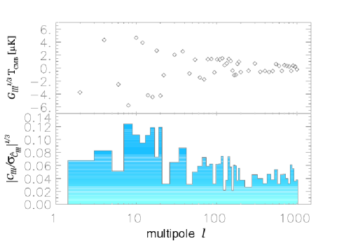
Figure 12: The CMB angular bispectrum in the ‘diagonal’ case ($G_{lll}^{1/3}$) from wiggly cosmic strings in a spatially flat model with cosmological parameters $\Omega_{\rm CDM}=0.3$, $\Omega_{\rm baryon}=0.05$, $\Omega_{\Lambda}=0.65$, and Hubble constant $H=0.65{\textrm{km}}{\textrm{s}}^{-1}{\textrm{Mpc}}^{-1}$ [upper panel]. In the lower panel we show the ratio of the signal to theoretical noise $|C_{lll}/\sigma_{\hat{C}_{lll}}|^{1/3}$ for different multipole indices. Normalization follows from fitting the power spectrum to the BOOMERANG and MAXIMA data.

The imprint of cosmic strings on the CMB is a combination of different effects. Prior to the time of recombination strings induce density and velocity fluctuations on the surrounding matter. During the period of last scattering these fluctuations are imprinted on the CMB through the Sachs-Wolfe effect, namely, temperature fluctuations arise because relic photons encounter a gravitational potential with spatially dependent depth. In addition to the Sachs-Wolfe effect, moving long strings drag the surrounding plasma and produce velocity fields that cause temperature anisotropies due to Doppler shifts. While a string segment by itself is a highly non-Gaussian object, fluctuations induced by string segments before recombination are a superposition of effects of many random strings stirring the primordial plasma. These fluctuations are thus expected to be Gaussian as a result of the central limit theorem.

As the universe becomes transparent, strings continue to leave their imprint on the CMB mainly due to the Kaiser & Stebbins [1984] effect. As we mentioned in previous sections, this effect results in line discontinuities in the temperature field of photons passing on opposite sides of a moving long string. However, this effect can result in non-Gaussian perturbations only on sufficiently small scales. This is because on scales larger than the characteristic inter-string separation at the time of the radiation-matter equality, the CMB temperature perturbations result from superposition of effects of many strings and are likely to be Gaussian. Avelino et al. [1998] applied several non-Gaussian tests to the perturbations seeded by cosmic strings. They found the density field distribution to be close to Gaussian on scales larger than $1.5(\Omega_{M}h^{2})^{-1}$ Mpc, where $\Omega_{M}$ is the fraction of cosmological matter density in baryons and CDM combined. Scales this small correspond to the multipole index of order $l\sim 10^{4}$.

V.4 CMB polarization

The possibility that the CMB be polarized was first discussed by Martin Rees in 1968, in the context of anisotropic universe models. In spite of his optimism, and after many attempts during more than thirty years, including some important upper limits [e.g., Keating, et al. 2001; Hedman, et al. 2001, 2002], there has been no positive detection of the polarization field until the DASI detection in September 2002 [Leitch et al. 2002; Kovac et al. 2002].

Unlike previous experiments, DASI reached the required sensitivity to make a sounding discovery on angular scales $\sim 0.\!\!^{\circ}5$. Along the same line, WMAP confirmed this detection with a full-sky coverage and polarization data on five different frequencies on angular scales bigger than $0.\!\!^{\circ}2$. Polarization is an important probe both for cosmological models and for the more recent history of our nearby Universe. It arises from the interactions of CMB photons with free electrons; hence, polarization can only be produced at the last scattering surface (its amplitude depends on the duration of the decoupling process) and, unlike temperature fluctuations, it is largely unaffected by variations of the gravitational potential after last scattering. Future measurements of polarization will thus provide a clean view of the inhomogeneities of the Universe at about 400,000 years after the Bang.

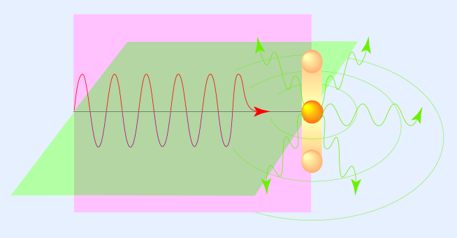
Figure 13: An electromagnetic linearly polarized wave (in red) oscillates in a given plane (in pink). Reaching an electron (orange ball) the wave induces the electron to also oscillate, making it emit radiation (in green). This resulting electromagnetic wave is concentrated essentially in the (green) plane orthogonal to the movement of the electron and it is polarized like the incident wave.

For understanding polarization, a couple of things should be clear. First, the energy of the photons is small compared to the mass of the electrons. Then, the CMB frequency does not change, since the electron recoil is negligible. Second, the change in the CMB polarization (i.e., the orientation of the oscillating electric field $\vec{\rm E}$ of the radiation) occurs due to a certain transition, called Thomson scattering. The transition probability per unit time is proportional to a combination of the old ($\hat{\epsilon}^{\rm~{}in}_{\alpha}$) and new ($\hat{\epsilon}^{\rm~{}out}_{\alpha}$) directions of polarization in the form $|\hat{\epsilon}^{\rm~{}in}_{\alpha}\cdot\hat{\epsilon}^{\rm~{}out}_{\alpha}|^{2}$. In other words, the initial direction of polarization will be favored. Third, an oscillating $\vec{\rm E}$ will push the electron to also oscillate; the latter can then be seen as a dipole (not to be confused with the CMB dipole), and dipole radiation emits preferentially perpendicularly to the direction of oscillation. These ‘rules’ will help us understand why the CMB should be linearly polarized agscien2 .

Previous to the recombination epoch, the radiation field is unpolarized. In unpolarized light the electric field can be decomposed into the two orthogonal directions (along, say, $\hat{x}$ and $\hat{z}$) perpendicular to the line of propagation ($\hat{y}$). The electric field along $\hat{\epsilon}^{\rm~{}in}_{\hat{z}}$ (suppose $\hat{z}$ is vertical) will make the electron oscillate also vertically. Hence, the dipolar radiation will be maximal over the horizontal $xy$-plane. Analogously, dipole radiation due to the electric field along $\hat{x}$ will be on the $yz$-plane. If we now look from the side (e.g., from $\hat{x}$, on the horizontal plane and perpendicularly to the incident direction $\hat{y}$) we will see a special kind of scattered radiation. From our position we cannot perceive the radiation that the electron oscillating along the $\hat{x}$ direction would emit, just because this radiation goes to the $yz$-plane, orthogonal to us. Then, it is as if only the vertical component ($\hat{\epsilon}^{\rm~{}in}_{\hat{z}}$) of the incoming electric field would cause the radiation we perceive. From the above rules we know that the highest probability for the polarization of the outgoing radiation $\hat{\epsilon}^{\rm~{}out}_{\alpha}$ will be to be aligned with the incoming one $\hat{\epsilon}^{\rm~{}in}_{\hat{z}}$, and therefore it follows that the outgoing radiation will be linearly polarized. Now, as both the chosen incoming direction and our position as observers were arbitrary, the result will not be modified if we change them. Thomson scattering will convert unpolarized radiation into linearly polarized one.

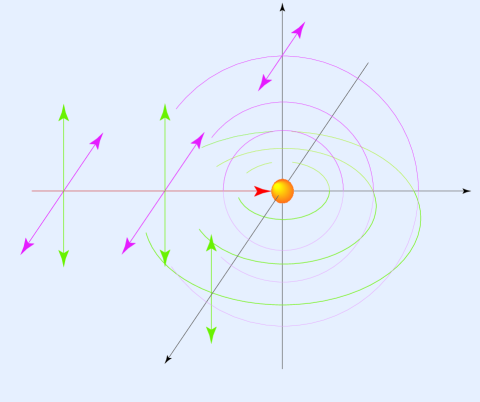
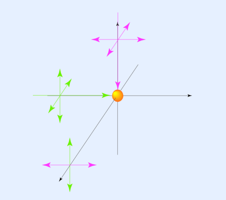
Figure 14: Left panel: non-polarized electromagnetic wave can be decomposed into the sum of two linearly-polarized waves, one along the line of sight (in pink), the other along a perpendicular direction (in green). Scattered radiation due to the first wave is contained in the plane orthogonal to the line of sight and cannot be detected. Only the second component (in green) reaches the observer and it is polarized as the incident wave. Right panel: when the charged particle receives non polarized waves from different directions (in green and pink), it will re-emit the radiation, polarized also along different directions, to the observer. If the original radiation is not isotropic (say, the pink arrow is bigger than the green one), then one of the resulting waves (in pink) will be slightly more intense than the other (in green), and the observer will perceive a net excess of linear polarization.

This however is not the end of the story. To get the total effect we need to consider all possible directions from which photons will come to interact with the target electron, and sum them up. We see easily that for an initial isotropic radiation distribution the individual contributions will cancel out: just from symmetry arguments, in a spherically symmetric configuration no direction is privileged, unlike the case of a net linear polarization which would select one particular direction.

Fortunately, we know the CMB is not exactly isotropic; to the millikelvin precision the dominant mode is dipolar. So, what about a CMB dipolar distribution ? Although spatial symmetry does not help us now, a dipole will not generate polarization either. Take, for example, the radiation incident onto the electron from the left to be more intense than the radiation incident from the right, with average intensities above and below (that’s a dipole); it then suffices to sum up all contributions to see that no net polarization survives. However, if the CMB has a quadrupolar variation in temperature (that it has, first discovered by COBE, to tens of $\mu$K precision) then there will be an excess of vertical polarization from left- and right-incident photons (assumed hotter than the mean) with respect to the horizontal one from top and bottom light (cooler). From any point of view, orthogonal contributions to the final polarization will be different, leaving a net linear polarization in the scattered radiation.

There is one more point to emphasize. Before recombination, ionized matter, electrons and radiation formed a single fluid. In it, the inertia was provided by massive nucleons whilst the pressure was that of radiation. And this fluid supported sound waves. In fact, the gravitational clumping tendency of the effective mass in the perturbations was resisted by the restoring radiation pressure, and therefore gravity-driven acoustic oscillations in both the fluid density and local velocity appeared.

Whereas the acoustic peaks in the temperature anisotropies correspond to the compression and rarefaction maxima of the oscillating plasma, the polarization field responds to the local quadrupole moment during the decoupling process. But this local quadrupole is mainly due to the Doppler shifts induced by the velocity field of the plasma [Zaldarriaga & Harari, 1995]. That is why we know with certainty that polarization shows the uncontaminated dynamics of the primordial seeds at recombination.

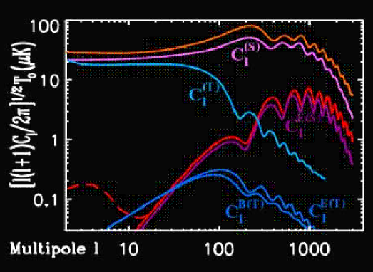
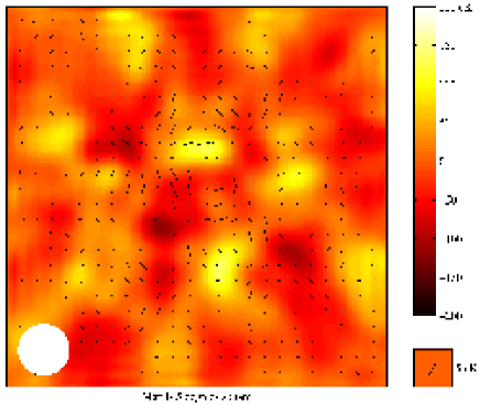
Figure 15: Left panel: CMB Polarization for two different models. Red and orange (unlabeled) curves are the angular spectra derived for a $\Lambda$CHDM model, both with (red dashed line) and without (red full line) reionization. The temperature anisotropy spectrum from scalar perturbations (proportional to $[C_{\ell}]^{1/2}$, orange curve) is virtually unchanged for both ionization histories. The polarization spectrum ($\propto[C^{\rm E(S)}_{\ell}]^{1/2}$, red curves), although indistinguishable for $\ell\hbox{ \raise 1.50696pt\hbox to0.0pt{$>$\hss}\lower 2.58334pt\hbox{$\sim$}\ }20$, dramatically changes for small $\ell$’s; in this model the Universe is reionized suddenly at low redshift with optical depth $\tau=0.05$ [recall, however, that recent first year data from the WMAP satellite indicates that $\tau=0.17\pm 0.04$]. Blue and violet curves represent a SCDM model but with a high tensor-mode amplitude, T/S=1 at the quadrupole ($\ell=2$) level, with scale-invariant spectral indices $n_{\rm S}=1$ and $n_{\rm T}=0$. Separate scalar (noted $C^{\rm(S)}_{\ell}$) and tensor ($C^{\rm(T)}_{\ell}$) contributions to temperature anisotropies are shown (top curves). Scalar modes only generate E-type polarization ($C^{\rm E(S)}_{\ell}$), which is smaller than the corresponding red curve of the $\Lambda$CHDM model both due to differences in the models (notably $\Lambda\not=0$ for the red curves) and due to the influence of tensors on the normalization at small $\ell$. E- and B-type polarization from tensor modes are also shown, respectively $C^{\rm E(T)}_{\ell}$ and $C^{\rm B(T)}_{\ell}$. Model spectra were computed with CMBFAST and are normalized to $\delta{\rm T}_{\ell=10}=27.9\mu{\rm K}$. Right panel: image of the intensity and polarization of the CMB made with the DASI telescope. The small temperature variations of the CMB are shown in false color, with yellow hot and red cold. The polarization at each spot in the image is shown by a black line. The length of the line shows the strength of the polarization and the orientation of the line indicates the direction in which the radiation is polarized. The size of the white spot in the lower left corner approximates the angular resolution of the observations.

Within standard recombination models the predicted level of linear polarization on large scales is tiny (see Figure 15): the quadrupole generated in the radiation distribution as the photons travel between successive scatterings is too small. Multiple scatterings make the plasma very homogeneous and only wavelengths that are small enough (big $\ell$’s) to produce anisotropies over the (rather short) mean free path of the photons will lead to a significant quadrupole, and thus also to polarization. Indeed, if the CMB photons last scattered at $z\sim 1100$, the SCDM model with $h=1$ predicts no more than 0.05 $\mu$K on scales greater than a few degrees. Hence, measuring polarization at these scales represents an experimental challenge.

However, CMB polarization increases remarkably around the degree-scale in standard models. In fact, for $\theta<1^{\circ}$ a bump with superimposed acoustic oscillations reaching $\sim 5\mu$K is generically forecasted. On these scales, like for the temperature anisotropies, the polarization field shows acoustic oscillations. However, polarization spectra are sharper: temperature fluctuations receive contributions from both density (dominant) and velocity perturbations and these, being out of phase in their oscillation, partially cancel each other. On the other hand, polarization is mainly produced by velocity gradients in the baryon-photon fluid before last scattering, which also explains why temperature and polarization peaks are located differently. Moreover, acoustic oscillations depend on the nature of the underlying perturbation; hence, we do not expect scalar acoustic sound-waves in the baryon-photon plasma, propagating with characteristic adiabatic sound speed $c_{\rm S}\sim c/\sqrt{3}$, close to that of an ideal radiative fluid, to produce the same peak-frequency as that produced by gravitational waves, which propagate with the speed of light $c$ (see Fig.15).

The main technical complication with polarization (characterized by a tensor field) is that it is not invariant under rotations around a given direction on the sky, unlike the temperature fluctuation that is described by a scalar quantity and invariant under such rotations. The level of linear polarization is conveniently expressed in terms of the Stokes parameters Q and U. It turns out that there is a clever combination of these parameters that results in scalar quantities (in contrast to the above noninvariant tensor description) but with different transformation properties under spatial inversions (parity transformations). Then, inspired by classical electromagnetism, any polarization pattern on the sky can be separated into ‘electric’ (scalar, unchanged under parity transformation) and ‘magnetic’ (pseudo-scalar, changes sign under parity) components (E- and B-type polarization, respectively).

V.4.1 CMB polarization from global defects

One then expands these different components in terms of spherical harmonics, very much like we did for temperature anisotropies, getting coefficients $a^{m}_{\ell}$ for E and B polarizations and, from these, the multipoles $C^{\rm E,B}_{\ell}$. The interesting thing is that (for symmetry reasons) scalar-density perturbations will not produce any B polarization (a pseudo-scalar), that is $C^{\rm B(S)}_{\ell}=0$. We see then that an unambiguous detection of some level of B-type fluctuations will be a signature of the existence (and of the amplitude) of a background of gravitational waves ! [Seljak & Zaldarriaga, 1997] (and, if present, also of rotational modes, like in models with topological defects).

Linear polarization is a symmetric and traceless 2x2 tensor that requires 2 parameters to fully describe it: $Q$, $U$ Stokes parameters. These depend on the orientation of the coordinate system on the sky. It is convenient to use $Q+iU$ and $Q-iU$ as the two independent combinations, which transform under right-handed rotation by an angle $\phi$ as $(Q+iU)^{\prime}=e^{-2i\phi}(Q+iU)$ and $(Q-iU)^{\prime}=e^{2i\phi}(Q-iU)$. These two quantities have spin-weights $2$ and $-2$ respectively and can be decomposed into spin $\pm 2$ spherical harmonics ${}_{\pm 2}Y_{lm}$

$$(Q+iU)(\hat{\hbox{\boldmath{$n$}}}) = \sum_{lm}a_{2,lm}\,{}_{2}Y_{lm}(\hat{\hbox{\boldmath{$n$}}})$$ (66)

$$(Q-iU)(\hat{\hbox{\boldmath{$n$}}}) = \sum_{lm}a_{-2,lm}\,{}_{-2}Y_{lm}(\hat{\hbox{\boldmath{$n$}}}).$$ (67)

Spin $s$ spherical harmonics form a complete orthonormal system for each value of $s$. Important property of spin-weighted basis: there exists spin raising and lowering operators $\;\raise 1.5pt\hbox{${}^{\prime}$}\hskip-6.0pt\partial\;$ and $\;\overline{\raise 1.5pt\hbox{${}^{\prime}$}\hskip-6.0pt\partial}\;$. By acting twice with a spin lowering and raising operator on $(Q+iU)$ and $(Q-iU)$ respectively one obtains quantities of spin 0, which are rotationally invariant. These quantities can be treated like the temperature and no ambiguities connected with the orientation of coordinate system on the sky will arise. Conversely, by acting with spin lowering and raising operators on usual harmonics spin $s$ harmonics can be written explicitly in terms of derivatives of the usual spherical harmonics. Their action on ${}_{\pm 2}Y_{lm}$ leads to

$$\;\overline{\raise 1.5pt\hbox{${}^{\prime}$}\hskip-6.0pt\partial}\;^{2}(Q+iU)(\hat{\hbox{\boldmath{$n$}}}) = \sum_{lm}\left({[l+2]!\over[l-2]!}\right)^{1/2}a_{2,lm}Y_{lm}(\hat{\hbox{\boldmath{$n$}}})$$ (68)

$$\;\raise 1.5pt\hbox{${}^{\prime}$}\hskip-6.0pt\partial\;^{2}(Q-iU)(\hat{\hbox{\boldmath{$n$}}}) = \sum_{lm}\left({[l+2]!\over[l-2]!}\right)^{1/2}a_{-2,lm}Y_{lm}(\hat{\hbox{\boldmath{$n$}}}).$$ (69)

With these definitions the expressions for the expansion coefficients of the two polarization variables become [Seljak & Zaldarriaga, 1997]

$$a_{2,lm} = \left({[l-2]!\over[l+2]!}\right)^{1/2}\int d\Omega\;Y_{lm}^{*}(\hat{\hbox{\boldmath{$n$}}})\;\overline{\raise 1.5pt\hbox{${}^{\prime}$}\hskip-6.0pt\partial}\;^{2}(Q+iU)(\hat{\hbox{\boldmath{$n$}}})$$ (70)

$$a_{-2,lm} = \left({[l-2]!\over[l+2]!}\right)^{1/2}\int d\Omega\;Y_{lm}^{*}(\hat{\hbox{\boldmath{$n$}}})\;\raise 1.5pt\hbox{${}^{\prime}$}\hskip-6.0pt\partial\;^{2}(Q-iU)(\hat{\hbox{\boldmath{$n$}}}).$$ (71)

Instead of $a_{2,lm}$, $a_{-2,lm}$ it is convenient to introduce their linear electric and magnetic combinations

$$a_{E,lm}=-{1\over 2}(a_{2,lm}+a_{-2,lm})\qquad a_{B,lm}={i\over 2}(a_{2,lm}-a_{-2,lm}).$$ (72)

These two behave differently under parity transformation: while $E$ remains unchanged $B$ changes the sign, in analogy with electric and magnetic fields.

To characterize the statistics of the CMB perturbations only four power spectra are needed, those for $X=T,E,B$ and the cross correlation between $T$ and $E$. The cross correlation between $B$ and $E$ or $B$ and $T$ vanishes because $B$ has the opposite parity of $T$ and $E$. As usual, the spectra are defined as the rotationally invariant quantities

$$C_{Xl}={1\over 2l+1}\sum_{m}\langle a_{X,lm}^{*}a_{X,lm}\rangle\qquad C_{Cl}={1\over 2l+1}\sum_{m}\langle a_{T,lm}^{*}a_{E,lm}\rangle$$ (73)

in terms of which on has

$$\langle a_{X,l^{\prime}m^{\prime}}^{*}a_{X,lm}\rangle = C_{Xl}\,\delta_{l^{\prime}l}\delta_{m^{\prime}m}$$ (74)

$$\langle a_{T,l^{\prime}m^{\prime}}^{*}a_{E,lm}\rangle = C_{Cl}\,\delta_{l^{\prime}l}\delta_{m^{\prime}m}$$ (75)

$$\langle a_{B,l^{\prime}m^{\prime}}^{*}a_{E,lm}\rangle = \langle a_{B,l^{\prime}m^{\prime}}^{*}a_{T,lm}\rangle=0.$$ (76)

According to what was said above, one expects some amount of polarization to be present in all possible cosmological models. However, symmetry breaking models giving rise to topological defects differ from inflationary models in several important aspects, two of which are the relative contributions from scalar, vector and tensor modes and the coherence of the seeds sourcing the perturbation equations. In the local cosmic string case one finds that in general scalar modes are dominant, if one compares to vector and tensor modes in the usual decomposition of perturbations. The situation with global topological defects is radically different and this leads to a very distinctive signature in the polarization field.

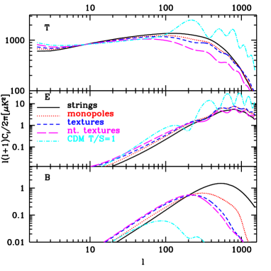
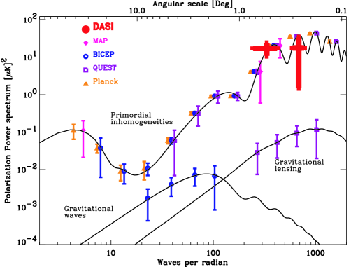
Figure 16: Left panel: Power spectra of temperature (T), electric type polarization (E) and magnetic type polarization (B) for global strings, monopoles, textures and nontopological textures [taken from Seljak. et al., 1997]. The corresponding spectra for a standard CDM model with $T/S=1$ is also shown for comparison. B polarization turns out to be notably larger for all global defects considered if compared to the corresponding predictions of inflationary models on small angular scales. Right panel: current and future polarization data by Hivon & Kamionkowski [2002]. Top curve shows the prediction for the polarization from primordial inhomogeneities produced by inflation. The large-angle bump in this curve is the enhancement from early star formation (reionization). The lower curves are for inflationary gravitational-wave and gravitational-lensing signals. Recently detected DASI data points are shown in red while the rest are expected data points for future experiments with more sensitivity.

Temperature and polarization spectra for various symmetry breaking models were calculated by Seljak, Pen & Turok [1997] and are shown in figure 16. Both electric and magnetic components of polarization are shown for a variety of global defects. They also plot for comparison the corresponding spectra in a typical inflationary model, namely, the standard CDM model ($h=0.5$, $\Omega=1$, $\Omega_{\rm baryon}=0.05$) but with equal amount of scalars and tensors perturbations (noted $T/S=1$) which maximizes the amount of B component from inflationary models. In all the models they assumed a standard reionization history. The most interesting feature they found is the large magnetic mode polarization, with a typical amplitude of $\sim 1\mu K$ on degree scales [exactly those scales probed by Hedman, et al., 2001]. For multipoles below $\ell\sim 100$ the contributions from $E$ and $B$ are roughly equal. This differs strongly from the inflationary model predictions, where $B$ is much smaller than $E$ on these scales even for the extreme case of $T/S\sim 1$. Inflationary models only generate scalar and tensor modes, while global defects also have a significant contribution from vector modes. As we mentioned above, scalar modes only generate $E$, vector modes predominantly generate $B$, while for tensor modes $E$ and $B$ are comparable with $B$ being somewhat smaller. Together this implies that B can be significantly larger in symmetry breaking models than in inflationary models. In figure 16 we also show the recent discovery of a tiny level of polarization by the DASI collaboration together with predictions for future experiments, assuming an inflationary origin for the temperature perturbation and polarization signals .

V.4.2 String lensing and CMB polarization

Recent studies have shown that in realistic models of inflation cosmic string formation seems quite natural in a post-inflationary preheating phase [Tkachev et al., 1998, Kasuya & Kawasaki, 1998]. So, even if the gross features on CMB maps are produced by a standard (e.g., inflationary) mechanism, the presence of defects, most particularly cosmic strings, could eventually leave a distinctive signature. One such feature could be found resorting to CMB polarization: the lens effect of a string on the small scale $E$-type polarization of the CMB induces a significant amount of $B$-type polarization along the line-of-sight [Zaldarriaga & Seljak, 1998; Benabed & Bernardeau 2000]. This is an effect analogous to the Kaiser-Stebbins effect for temperature maps.

In the inflationary scenario, scalar density perturbations generate a scalar polarization pattern, given by $E$-type polarization, while tensor modes have the ability to induce both $E$ and $B$ types of polarization. However, tensor modes contribute little on very small angular scales in these models. So, if one considers, say, a standard $\Lambda\mathrm{CDM}$ model, only scalar primary perturbations will be present without defects. But if a few strings are left from a very early epoch, by studying the patch of the sky where they are localized, a distinctive signature could come to light.

In the small angular scale limit, in real space and in terms of the Stokes parameters $Q$ and $U$ one can express the $E$ and $B$ fields as follows

$$E\equiv\Delta^{-1}[({\partial x}^{2}-{\partial y}^{2})\,Q+2{\partial x}{\partial y}\,U],$$ (77)

$$B\equiv\Delta^{-1}[({\partial x}^{2}-{\partial y}^{2})\,U-2{\partial x}{\partial y}\,Q].$$ (78)

The polarization vector is parallel transported along the geodesics. The lens affects the polarization by displacing the apparent position of the polarized light source. Hence, the observed Stokes parameters $\hat{Q}$ and $\hat{U}$ are given in terms of the primary (unlensed) ones by: $\hat{Q}(\vec{\alpha})=Q(\vec{\alpha}+\vec{\xi})\,{\rm~{}and~{}}\,\hat{U}(\vec{\alpha})=U(\vec{\alpha}+\vec{\xi})$. The displacement $\vec{\xi}$ is given by the integration of the gravitational potential along the line–of–sights. Of course, here the ‘potential’ acting as lens is the cosmic string whose effect on the polarization field we want to study.

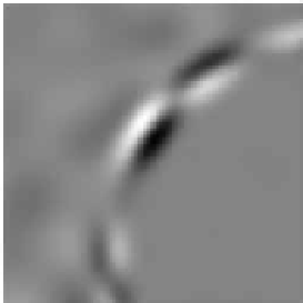
Figure 17: Simulations for the $B$ field in the case of a circular loop. The angular size of the figure is $50^{\prime}\times 50^{\prime}$. The resolution is 5’ (left) and 1.2’ (right). The discontinuity in the $B$ field is sharper the better the resolution. Weak lensing of CMB photons passing relatively apart from the position of the string core are apparent as faint patches outside of the string loop on the left panel. [Benabed & Bernardeau 2000].

In the case of a straight string which is aligned along the $y$ axis, the deflection angle (or half of the deficit angle) is $4\pi G\mu$ [Vilenkin & Shellard, 2000] and this yields a displacement $\xi_{x}=\pm\xi_{0}$ with

$$\xi_{0}=4\pi G\mu{\mathcal{D}}_{\textrm{lss,s}}/{\mathcal{D}}_{\textrm{s,us}}$$ (79)

with no displacement along the $y$ axis. ${\mathcal{D}}_{\textrm{lss,s}}$ and ${\mathcal{D}}_{\textrm{s,us}}$ are the cosmological angular distances between the last scattering surface and the string, and between the string and us, respectively. They can be computed, in an Einstein-de Sitter universe (critical density, just dust and no $\Lambda$), from

$${\mathcal{D}}_{\textrm{}}(z_{1},z_{2})={2c\over H_{0}}{1\over 1+z_{2}}[(1+z_{1})^{-1/2}-(1+z_{2})^{-1/2}]$$ (80)

by taking $z_{1}=0$ for us and $z_{2}\simeq 1000$ for the last scattering surface; see [Bartelmann & Schneider, 2001]. For the usual case in which the redshift of the string $z_{\rm s}$ is well below the $z_{\textrm{lss}}$ one has ${\mathcal{D}}_{\textrm{lss,s}}/{\mathcal{D}}_{\textrm{lss,us}}\simeq 1/\sqrt{1+z_{\rm s}}$. Taking this ratio of order 1/2 (i.e., distance from us to the last scattering surface equal to twice that from the string to the last scattering surface) yields $z_{\rm s}\simeq 3$. Plugging in some numbers, for typical GUT strings on has $G\mu\simeq 10^{-6}$ and so the typical expected displacement is about less than 10 arc seconds. Benabed & Bernardeau [2000] compute the resulting $B$ component of the polarization and find that the effect is entirely due to the discontinuity induced by the string, being nonzero just along the string itself. This clearly limits the observability of the effect to extremely high resolution detectors, possibly post-Planck ones.

The situation for circular strings is different. As shown by de Laix & Vachaspati [1996] the lens effect of such a string, when facing the observer, is equivalent to the one of a static linear mass distribution. Considering then a loop centered at the origin of the coordinate system, the displacement field can be expressed very simply: observing in a direction through the loop, $\vec{\xi}$ has to vanish, while outside of the loop the displacement decreases as ${\alpha_{l}}/{\alpha}$, i.e., inversely proportional to the angle. One then has [Benabed & Bernardeau, 2000]

$$\vec{\xi}(\vec{\alpha})=-2\xi_{0}{\alpha_{l}\over\alpha^{2}}\vec{\alpha}\quad{\rm~{}with~{}}\quad\alpha>\alpha_{l},$$ (81)

where $\alpha_{l}$ is the loop radius.

This ansatz for the displacement, once plugged into the above equations, yields the $B$ field shown in both panels of Figure 17. A weak lensing effect is barely distinguishable outside the string loop, while the strong lensing of those photons traveling close enough to the string is the most clear signature, specially for the high resolution simulation. One can check that the hot and cold spots along the string profile have roughly the same size as for the polarization field in the absence of the string loop. The simulations performed show a clear feature in the maps, although limited to low resolutions this can well be confused with other secondary polarization sources. It is well known that point radio sources and synchrotron emission from our galaxy may contribute to the foreground [de Zotti et al. 1999] and are polarized at a 10 % level. Also lensing from large scale structure and dust could add to the problem.

VI Cosmic defects in perspective

Cosmic defects have proved very interesting and fruitful in high–energy physics and astrophysics. Their generic production in grand unified theories has made defects an active field of research for over two decades. Many of the interesting subjects now associated with defects were only briefly mentioned in these notes, like the internal structure of defects –leading to persistent currents in their cores– and, as a consequence, the possible generation of primordial magnetic fields. Also, primordial gravitational waves, extremely high–energy phenomena associated to cosmic rays and uhecrons, electroweak baryogenesis and, finally, the very active condensed-matter–cosmology interface, dubbed cosmos in the lab, equally –and unjustly– received no attention [compensate for this with references like Vilenkin & Shellard, 2000; Hindmarsh & Kibble, 1995; Kibble, 2002; Gangui, 2001b, for example – yes, in that order.]. With regards to the most transparent test of current cosmology, namely the CMB and matter power spectra, (not so) recent investigations have pointed out severe problems in virtually all models where cosmic defects are the main source of the seeds of structure in the universe. In the case of cosmic strings, however, these bad news were reached by the use of non–negligible, albeit well–founded, approximations in order to cope with the limited range of realistic defect simulations [bad or good news, depending on which side you are.] Although the whole method of unequal time correlators employed by most of the groups can be regarded as a good approximation to reality during both the matter and radiation eras, the important transition in between must be looked at more carefully, as the above–mentioned correlators do not scale as expected. Recent, full Boltzmann analyses aiming to solve this handicap are in progress [e.g., Landriau & Shellard, 2002, 2003] and already producing interesting results.

References

- (1) Abrikosov, A. A. [1957], Sov. Phys. JETP 5, 1174 [Zh. Eksp. Teor. Fiz. 32, 1442 (1957)]
- (2) Achúcarro, A. & Vachaspati, T. [2000], Phys. Rept. 327, 347-426; Phys. Rept. 327, 427. [hep-ph/9904229]
- (3) Albrecht, A., Battye, R. & Robinson, J. [1997], Phys. Rev. Lett. 79, 4736.; Phys. Rev. D59, 023508 (1998).
- (4) Albrecht, A., Coulson, D., Ferreira, P. & Magueijo, J. [1995], Imperial Preprint /TP/94–95/30.
- (5) Alexander, S., Brandenberger, R., Easther, R. & Sornborger, A. [1999], hep-ph/9903254.
- (6) Avelino, P.P. & Martins, C.J.A.P. [2000], Phys. Rev. Lett. 85, 1370.
- (7) Avelino, P.P., Shellard, E.P.S., Wu, J.H.P. & Allen, B. [1998], Astrophys. J. 507, L101.
- (8) Bartelmann, M. & Schneider, P. [2001], Phys. Rep. 340, 291.
- (9) Battye, R. A., Bucher, M. & Spergel, D. [1999], astro-ph/9908047 .
- (10) Battye, R. & Weller, J. [2000], Phys. Rev. D61, 043501.
- (11) Benabed, K. & Bernardeau, F. [2000], Phys. Rev. D61, 123510.
- (12) Bennett, C., et al. [2003], astro-ph/0302207.
- (13) Bennett, D.P. & Rhie, S.H. [1990], Phys. Rev. Lett. 65, 1709.
- (14) Bennett, D.P. & Rhie, S.H. [1993], Ap. J. Lett. 406, L7.
- (15) Bennett, D.P., Rhie, S.H. & Weinberg, D.H. [1993], preprint.
- (16) Borrill, J., et al. [1994], Phys. Rev. D50, 2469.
- (17) Bouchet, F.R., Peter, P., Riazuelo, A. & Sakellariadou, M. [2001], preprint astro-ph/0005022.
- (18) Brandenberger, R. [1993], Topological Defects and Structure Formation, EPFL lectures, Lausanne, Switzerland.
- (19) Bunkov, Y. & Godfrin, H. [2000], (editors) Proceedings of the NATO-ASI on topological defects and non-equilibrium dynamics of symmetry breaking phase transitions (Kluwer, Dordrecht).
- (20) Callan, C. & Coleman, S. [1977], Phys. Rev. D16, 1762.
- (21) Carter, B, [1990], Phys. Rev. D41, 3869.
- (22) Carter, B. [1997], Tlaxcala lecture notes, hep-th/9705172.
- (23) Carter, B., Peter, P. & Gangui, A. [1997], Phys. Rev. D55, 4647. [hep-ph/9609401];
- (24) Contaldi, C., Hindmarsh, M. & Magueijo, J. [1999], Phys. Rev. Lett. 82 2034.
- (25) Copeland, E. [1993], in The physical universe: The interface between cosmology, astrophysics and particle physics, eds. Barrow, J.D., et al. (Sringer–Verlag).
- (26) Cowie, L. & Hu, E. [1987], Ap. J.318 L33.
- (27) Davis, R. L. [1987], Phys. Rev. D 35, 3705.
- (28) Davis, R.L. & Shellard, E.P.S. [1988], Phys. Lett. B207, 404.
- (29) de Bernardis, P. et al. [2000], Nature 404, 995 [astro-ph/0004404]
- (30) de Laix, A.A. & Vachaspati, T. [1996], Phys. Rev. D54, 4780.
- (31) de Zotti, G. et al.[1999], astro–ph/9908058.
- (32) Dolan, L. & Jackiw, R. [1974], Phys. Rev. D9, 3320.
- (33) Durrer, R. [2000], in Moriond meeting on Energy Densities in the Universe, astro-ph/0003363 .
- (34) Durrer, R., Gangui, A. & Sakellariadou, M. [1996], Phys. Rev. Lett. 76, 579. [astro-ph/9507035].
- (35) Durrer, R., Kunz, M. & Melchiorri, A. [2002], Phys.Rept. 364 (2002) 1-81. [astro-ph/0110348].
- (36) Durrer, R. & Zhou, Z.H. [1995], Zürich University Preprint, ZH–TH19/95, astro–ph/9508016.
- (37) Dvali, G., Liu, H. & Vachaspati, T. [1998], Phys. Rev. Lett. 80, 2281.
- (38) Gangui, A. [2001], Science 291, 837.
- (39) Gangui, A. [2003], Science 299, 1333.
- (40) Gangui, A. [2001b], Topological Defects in Cosmology, Lecture Notes for the First Bolivian School on Cosmology, in press [astro-ph/0110285].
- (41) Gangui, A., Lucchin, F., Matarrese, S. & Mollerach, S. [1994], Ap. J. 430, 447.
- (42) Gangui, A. & Martin, J. [2000a], Mon. Not. R. Astron. Soc. 313, 323. [astro-ph/9908009]
- (43) Gangui, A. & Martin, J. [2000b], Phys. Rev. D62, 103004. [astro-ph/0001361]
- (44) Gangui, A. & Mollerach, S. [1996], Phys. Rev. D54, 4750-4756. [astro-ph/9601069]
- (45) Gangui, A. & Peter, P. [1998], Cosmological and Astrophysical Implications of Superconducting Cosmic Strings and Vortons, in Proceedings of the XXXIIIrd Rencontres de Moriond on ‘Fundamental Parameters in Cosmology’, pages 19-24, Editors: J. Tran Thanh Van et al., Editions Frontières, 1998.
- (46) Gangui, A., Peter, P. & Boehm, C. [1998], Phys. Rev. D57, 2580. [hep-ph/9705204]
- (47) Gangui, A., Pogosian, L. & Winitzki, S. [2001a], New Astronomy Reviews 46, 681-691 (2002). [astro-ph/0112145]
- (48) Gangui, A., Pogosian, L. & Winitzki, S. [2001b], Phys. Rev. D64, 043001.
- (49) Goto, T. [1971], Prog. Theor. Phys. 46, 1560.
- (50) Gott, R. [1985], Ap. J., 288, 422.
- (51) Guth, A.H. & Weinberg, E. [1983], Nucl. Phys. B212, 321.
- (52) Hanany, S., et al, Astrophys. J. Lett. accepted (2000), astro-ph/0005123; Jaffe, A.H., et al, astro-ph/0007333.
- (53) Halverson, N.W. et al, preprint astro-ph/0104489.
- (54) Hedman, M., Barkats, D., Gundersen, J. Staggs, S. & Winstein, B. [2001], Ap. J., 548, L111-L114 [astro-ph/0010592]; Hedman, M. et al. [2002], Astrophys. J. 573, L73 (2002).
- (55) Higgs, P. [1964], Phys. Lett. 12, 132.
- (56) Hilton, P.J. [1953], Introduction to homotopy theory (Cambridge: Cambridge University Press).
- (57) Hindmarsh, M.B. & Kibble, T.W.B. [1995], Rept. Prog. Phys. 58, 477-562 [hep-ph/9411342].
- (58) Hivon, E. & Kamionkowski, M. [2002], Science 298, 1349.
- (59) Hu, W., Spergel, D. & White, M. [1997], Phys. Rev. D55, 3288-3302.
- (60) Kaiser, N. & Stebbins, A. [1984], Nature 310, 391.
- (61) Kasuya, S. & Kawasaki, M, [1998], Phys. Rev. D58, 083516.
- (62) Keating, B. et al. [2001], Astrophys. J. 560, L1 (2001).
- (63) Kibble, T.W.B. [1976], J. Phys. A9, 1387.
- (64) Kibble, T.W.B. [1980], Phys. Rep. 67, 183.
- (65) Kibble, T.W.B. [1985], Nucl. Phys. B252, 227; B261, 750 (1986).
- (66) Kibble, T.W.B. [2002], Lectures at NATO ASI “Patterns of symmetry breaking”, Cracow [cond-mat/0211110].
- (67) Kibble, T.W.B., Lazarides, G. & Shafi, Q. [1982], Phys. Lett. B113, 237.
- (68) Kirzhnits, D.A. & Linde, A.D. [1974], Sov. Phys. JETP 40, 628.
- (69) Kirzhnits, D.A. & Linde, A.D. [1976], Ann. Phys. 101, 195.
- (70) Kogut, A., et al. [2003], astro-ph/0302213.
- (71) Kolb, E.W. & Turner, M.S. [1990] The Early Universe (New York: Addison–Wesley).
- (72) Komatsu, E. & Spergel, D. [2000], preprint astro-ph/0005036;
- (73) Kovac, J. et al. [2002], Nature 420, 772-787. [astro-ph/0209478]
- (74) Lemperière, Y. & Shellard, E.P.S. [2002], preprint hep-ph/0207199 .
- (75) Landriau, M. & Shellard, E.P.S. [2002], preprint astro-ph/0208540 .
- (76) Landriau, M. & Shellard, E.P.S. [2003], preprint astro-ph/0302166 .
- (77) Langacker, P. & Pi, S.–Y. [1980], Phys. Rev. Lett. 45, 1.
- (78) Langer, S. [1992], in Solids far from equilibrium, Godrèche, C., ed. (Cambridge: Cambridge University Press).
- (79) Leitch, E.M. et al. [2002], Nature 420, 763-771. astro-ph/0209476
- (80) Liddle, A. [1995], Phys. Rev. D51, 5347-5351.
- (81) Linde, A.D. [1983b], Nucl. Phys. B216, 421.
- (82) Linet, B. [1986], Phys. Rev. D33 1833.
- (83) Magueijo, J. , Albrecht, A. , Ferreira, P. & Coulson, D. [1996], Phys. Rev. D54, 3727-3744.
- (84) Magueijo, J. & Brandenberger, R. [2000], Iran lectures on cosmic defects, astro-ph/0002030.
- (85) Magueijo, J. & Ferreira, P. [1997], Phys. Rev. D55, 3358.
- (86) Martins, C.J.A.P. & Shellard, E.P.S. [1996], Phys. Rev. D54 2535.
- (87) Martins, C.J.A.P. & Shellard, E.P.S. [2000], hep-ph/0003298
- (88) Mermin, M. [1979] , Rev. Mod. Phys. 51, 591.
- (89) Nambu, Y. [1970], in Proc. Int. Conf. on Symmetries and Quark Models, ed. Chand, R. (New York: Gordon and Breach).
- (90) Notzold, D. [1991], Phys. Rev. D43, R961.
- (91) Page, L., et al. [2003], astro-ph/0302220.
- (92) Peebles, P.J.E. & Ratra, B. [2002], Rev. Mod. Phys. (in press) astro-ph/0207347 .
- (93) Pen, U.-L., Seljak, U. & Turok, N. [1997], Phys. Rev. Lett. 79, 1611-1614.
- (94) Pen, U.–L., Spergel, D.N. & Turok, N. [1994], Phys. Rev. D49, 692.
- (95) Perlmutter, S., et al. [1999], Astrophys. J. 517, 565.
- (96) Pogosian, L. [2001], Int. J. Mod. Phys. A16S1C . astro-ph/0009307.
- (97) Pogosian, L. & Vachaspati, T. [1999], Phys. Rev. D60, 083504.
- (98) Pogosian, L. & Vachaspati, T. [2000], Phys. Rev. D62, 105005.
- (99) Preskill, J. [1979], Phys. Rev. Lett. 43, 1365.
- (100) Rajaraman, R. [1982], Solitons and instantons (Amsterdam: North–Holland).
- (101) Riess, A.G, et al. [1998], Astron.J. 116, 1009-1038. astro-ph/9805201
- (102) Sachs, R. & Wolfe, A. [1967], Ap. J. 147, 73.
- (103) Sazhin, M., et al. [2003], to appear in MNRAS. [astro-ph/0302547]
- (104) Scaramella, R. & Vittorio, N. [1991], Ap. J. 375, 439.
- (105) Scaramella, R. & Vittorio, N. [1993], M.N.R.A.S. 263, L17.
- (106) Seljak, U., Pen, U.-L. & Turok, N. [1997], Phys.Rev.Lett. 79 1615-1618.
- (107) Seljak, U. & Zaldarriaga, M. [1996], Astrophys. J. 469, 437.
- (108) Seljak, U. & Zaldarriaga, M. [1997], Phys. Rev. Lett. 78, 2054.
- (109) Silk, J. & Vilenkin, A. [1984], Phys. Rev. Lett. 53, 1700.
- (110) Steenrod, N. [1951], Topology of Fibre Bundles (Princeton: Princeton University Press).
- (111) Tkachev, I., Khlebnikov, S., Kofman, L. & Linde, A. [1998], Phys.Lett. B440, 262-268.
- (112) Turok, N. [1989], Phys. Rev. Lett. 63, 2625.
- (113) Turok, N. [1996], Phys. Rev. Lett. 77, 4138-4141; Phys. Rev. D54, 3686-3689
- (114) Turok, N., Pen, U.-L. & Seljak, U. [1998], Phys. Rev. D58, 023506.
- (115) Turok, N. & Spergel, D.N. [1990], Phys. Rev. Lett. 64, 2736.
- (116) Turok, N. & Zadrozny, J. [1990], Phys. Rev. Lett. 65, 2331.
- (117) Vachaspati, T. [2001], ICTP summer school lectures, hep-ph/0101270.
- (118) Vachaspati, T. & Vilenkin, A. [1991], Phys. Rev. Lett. 67, 1057.
- (119) Veeraraghavan, S. & Stebbins, A. [1990], Ap. J. 365, 37.
- (120) Vilenkin, A. [1981], Phys. Rev. D23, 852.
- (121) Vilenkin, A. [1983], Phys. Rev. D27, 2848.
- (122) Vilenkin, A. [1984], Phys. Rev. Lett. 53, 1016.
- (123) Vilenkin, A. [1985], Phys. Rep. 121, 263.
- (124) Vilenkin, A [1990], Phys. Rev. D41, 3038.
- (125) Vilenkin, A. & Shellard, E.P.S. [2000], Cosmic Strings and other Topological Defects, 2nd edition, (Cambridge: CUP).
- (126) Vollick, D.N. [1992], Phys. Rev. D45, 1884.
- (127) Walker, P.N., et al. [1991], Ap. J. 376, 51. Wang, L. & Kamionkowski, M. [2000], Phys. Rev. D61, 063504.
- (128) Weinberg, S. [1974], Phys. Rev. D9, 3357.
- (129) Wu, J.-H.P. et al, preprint astro-ph/9812156.
- (130) Zaldarriaga, M. & Harari, D. [1995], Phys. Rev. D52, 3276.
- (131) Zaldarriaga, M. & Seljak, U. [1998], Phys. Rev. D58, 023003.
- (132) Zel’dovich, Ya. B., I. Yu. Kobzarev & L. B. Okun [1974], Zh. Eksp. Teor. Fiz. 67, 3 [Sov. Phys. JETP 40, 1 (1975)].