Relativistic Magnetohydrodynamics with Application to Gamma-Ray Burst Outflows: I. Theory and Semianalytic Trans-Alfvénic Solutions

Abstract

We present a general formulation of special-relativistic magnetohydrodynamics and derive exact radially self-similar solutions for axisymmetric outflows from strongly magnetized, rotating compact objects. We generalize previous work by including thermal effects and analyze in detail the various forces that guide, accelerate, and collimate the flow. We demonstrate that, under the assumptions of a quasi-steady poloidal magnetic field and of a highly relativistic poloidal velocity, the equations become effectively time-independent and the motion can be described as a frozen pulse. We concentrate on trans-Alfvénic solutions and consider outflows that are super-Alfvénic throughout in the companion paper. Our results are applicable to relativistic jets in gamma-ray burst (GRB) sources, active galactic nuclei, and microquasars, but our discussion focuses on GRBs. We envision the outflows in this case to initially consist of a hot and optically thick mixture of baryons, electron-positron pairs, and photons. We show that the flow is at first accelerated thermally but that the bulk of the acceleration is magnetic, with the asymptotic Lorentz factor corresponding to a rough equipartition between the Poynting and kinetic-energy fluxes (i.e., $\sim 50\%$ of the injected total energy is converted into baryonic kinetic energy). The electromagnetic forces also strongly collimate the flow, giving rise to an asymptotically cylindrical structure.

Submitted to ApJ on March 19, 2003 Submitted to ApJ on March 19, 2003

1 Introduction

The acceleration and collimation of powerful bipolar outflows and jets in a variety of astronomical settings are often attributed to the action of magnetic fields (see, e.g., Livio 2000 and Königl & Pudritz 2000 for reviews). The commonly invoked scenario is that magnetic field lines threading a rotating compact object or its surrounding accretion disk can efficiently tap the rotational energy of the source and accelerate gas to supersonic speeds through centrifugal and/or magnetic pressure-gradient forces. It is argued that the hoop stresses of the twisted field lines can account for the narrowness of many jets and that, in many cases, alternative production mechanisms (such as thermal driving) can be excluded on observational grounds.

Although numerical simulations have provided useful insights into various aspects of hydromagnetic jet production, practical limitations have necessitated complementing this approach with analytic studies. Owing to the complexity of the problem, the most general semianalytic solutions obtained so far have been time-independent and self-similar, patterned after the pioneering disk-outflow solutions of Blandford & Payne (1982). The advantage of pursuing such solutions is that they are exact and self-consistent, and that they can be systematically classified (e.g., Vlahakis & Tsinganos, 1998). Furthermore, these solutions are evidently rich enough to capture most of the relevant physics, as corroborated by numerical calculations (e.g., Ouyed & Pudritz, 1997; Ustyugova et al., 1999; Krasnopolsky, Li, & Blandford, 1999).

Almost all of the previous semianalytic work on jet magnetohydrodynamics (MHD) was done in the Newtonian limit of nonrelativistic bulk and random speeds. Relativistic outflows are, however, observed quite commonly in Nature — with examples including active galactic nuclei (AGNs), Galactic superluminal sources (often referred to as “microquasars”), pulsars, and gamma-ray bursts (GRBs)— and in many of these cases magnetic fields are again implicated as the main driving and collimation mechanism (e.g., Blandford, 2002a). This provides a motivation for generalizing the Newtonian self-similar outflow solutions, although it is readily seen that this cannot be done in a totally straightforward manner. For one thing, special-relativistic MHD (unlike the nonrelativistic theory) involves a characteristic speed (the speed of light $c$), which precludes the incorporation of gravity into the self-similar equations and a simple matching of the outflow solution to a particular (e.g., Keplerian) disk rotation law. Furthermore, again in contrast with the nonrelativistic formulation, the displacement current and the charge density cannot be neglected in the constitutive equations (which now must also satisfy relativistic covariance).

Despite the aforementioned complications, Li, Chiueh, & Begelman (1992) and Contopoulos (1994) succeeded in generalizing the “cold,” radially self-similar solutions of Blandford & Payne (1982) to the relativistic regime. Their solutions are characterized by the thermal pressure playing a negligible role in the flow acceleration and by the flow being trans-Alfvénic: the poloidal speed is less than the poloidal component of the Alfvén speed at the base of the flow, and comes to exceed it further up. Our aim in this paper is to further generalize these solutions to the “hot” relativistic case — i.e., we allow both the bulk and the random speeds to be relativistic. This is motivated primarily by the desire to apply these solutions to GRB outflows, in which thermal driving by an optically thick, hot “fireball” composed primarily of radiation and electron-positron pairs could play a role. In fact, most previous models of GRB outflows were purely hydrodynamical and included only thermal driving (see, e.g., Piran 1999 for a review). It has subsequently been realized that energy deposition by annihilating neutrinos, which had been one of the main proposed heating mechanisms, would typically be inefficient (e.g., Di Matteo, Perna, & Narayan, 2002), and it was, furthermore, argued (Daigne & Mochkovitch, 2002) that only a small fraction ($\lesssim 1\%$) of the energy deposited in the source could be in thermal form to avoid generating strong photospheric emission in the outflow (for which there has been no observational evidence). For these (and other) reasons, it is now believed that magnetic fields play the dominant role in the driving of GRB jets (e.g., Mészáros 2002). Nevertheless, some thermal energy injection, either by neutrinos or by magnetic energy dissipation, is likely to take place (e.g., Narayan, Paczyński, & Piran, 1992; Mészáros, Laguna, & Rees, 1993), and, as we show in §4.1, even if it contributes only a small fraction of the initial energy flux in the flow, it can dominate the early phase of the acceleration. There are indications that thermal energy deposition at the source may also contribute to the initial acceleration of relativistic jets in AGNs (e.g., Melia, Liu, & Fatuzzo 2002; N. Vlahakis & A. Königl, in preparation). It thus appears that, to fully understand the nature of such jets, it is necessary to model them in terms of a “hot” MHD outflow.

The ability of large-scale, ordered magnetic fields to guide, collimate, and accelerate relativistic outflows has been previously discussed by various authors (including, in the GRB context, Usov 1994, Thompson 1994; Mészáros & Rees 1997, Katz 1997, Kluźniak & Ruderman 1998, Lyutikov & Blackman 2001, and Drenkhahn & Spruit 2002). These discussions, however, did not include exact solutions from which detailed quantitative estimates could be made. In a previous paper, Vlahakis & Königl (2001, hereafter VK01) presented a semianalytic self-similar solution of the “hot” relativistic MHD equations and applied it to the interpretation of GRBs. The full formalism underlying this solution is described in the present paper, where we also analyze its dependence on the relevant physical parameters and compare it with other characteristic solutions of trans-Alfvénic flows. This discussion is extended in the companion paper (Vlahakis & Königl 2003, hereafter Paper II), where we focus on super-Alfvénic flows.

The self-similar solutions that we derive correspond to ordered magnetic field configurations in the ideal-MHD limit. Although it is quite conceivable that the fields that drive the flow from a differentially rotating star or disk are at least in part small-scale and disordered, the statistical (temporal and spatial) averages of such fields could in principle have a similar effect to that of large-scale, ordered field configurations in providing both acceleration (Heinz & Begelman, 2000) and collimation (Li, 2002). The applicability of ideal MHD to the acceleration of ultrarelativistic flows has been questioned by Blandford (2002b; see also Lyutikov & Blandford 2002), who proposed instead a force-free electromagnetic formulation. We note in this connection that a force-free behavior can be recovered from the relativistic MHD formulation as a limiting case of negligible particle inertia. Furthermore, electromagnetic energy dissipation — perhaps the strongest argument against the ideal-MHD modeling framework — has been claimed to lead, on its own, to an efficient conversion of Poynting flux into a highly relativistic bulk motion (e.g., Drenkhahn & Spruit, 2002). Our ideal-MHD solutions may thus be regarded as a first step toward a more comprehensive theory in which dissipation effects will be taken into account (and possibly further enhance the effectiveness of the magnetic acceleration process).

Although the formulation presented in this paper is quite general, the main application that we consider is to GRB sources. For definiteness, we adopt the “internal shock” scenario for the origin of the prompt high-energy emission in GRBs (e.g., Piran, 1999). Considerations involving variability time scales (as interpreted in the context of this picture) as well as source energetics support the identification of an accretion disk around a newly formed black hole as the source of the GRB outflow (e.g., Piran, 2001a); accordingly, we concentrate on modeling jets from accretion disks. However, our solutions should be at least qualitatively applicable also to other source configurations, such as a rapidly spinning neutron star (e.g., Usov, 1994; Kluźniak & Ruderman, 1998) or a rotating, magnetically threaded black hole (e.g., Blandford & Znajek, 1977; van Putten, 2001). Since GRB outflows have a limited duration (the value of which is plausibly related to the disk accretion time), a naive application of a steady-state similarity solution is not warranted. In previous, purely hydrodynamical models of GRB outflows, this difficulty was circumvented by applying the so-called “frozen pulse” approximation (Piran, Shemi, & Narayan, 1993). In this paper we prove (§2.1) that this approximation can be generalized to the relativistic MHD regime, but we also demonstrate (§4.1.1) how any inherent time dependence can be recovered.

The plan of the paper is as follows. In §2 we present the equations of time-dependent relativistic MHD, simplify them using the frozen-pulse approximation, and discuss what effect each of the various forces acting on the plasma has on the flow acceleration and collimation. In §3 we describe the $r$ self-similar model and in §4 we give the results of the numerical integration of the model equations. We discuss general implications of this work to GRB sources and other relativistic jet sources in §5, where we also summarize our conclusions.

2 The Relativistic MHD Formulation

2.1 Governing Equations

The stress-energy tensor of relativistic MHD consists of three parts — matter (subscript M), radiation (subscript R) and electromagnetic fields (subscript EM): $T^{\kappa\nu}=T^{\kappa\nu}_{\rm M}+T^{\kappa\nu}_{\rm R}+T^{\kappa\nu}_{\rm EM}$ ($\kappa\,,\nu=0,1,2,3$). The matter component is given by $T^{\kappa\nu}_{\rm M}=\left(\rho_{\rm M}+P_{\rm M}/c^{2}\right)U^{\kappa}U^{\nu}+P_{\rm M}\eta^{\kappa\nu}$, where $\rho_{\rm M}c^{2}=\rho_{0}c^{2}+\rho_{0}e_{\rm M}$ is the total comoving matter energy density, $P_{\rm M}$ is the particle pressure, $U^{\nu}=\left(\gamma c,\gamma\boldsymbol{V}\right)$ is the fluid four-velocity, and $\eta^{\kappa\nu}={\rm diag}\left(-1\,1\,1\,1\right)$ is the metric tensor (assuming a flat spacetime and Cartesian space coordinates $x_{j},\ j=1,2,3$). Here $\rho_{0}$ is the baryon rest-mass density, $\rho_{0}e_{\rm M}=P_{\rm M}/(\Gamma-1)$ is the internal energy density, with $\Gamma$ denoting the polytropic index ($=4/3$ or $5/3$ in the limit of an ultrarelativistic or a nonrelativistic temperature, respectively), $\boldsymbol{V}$ is the three-velocity measured in the frame of the central object, and $\gamma=1/(1-V^{2}/c^{2})^{1/2}$ is the Lorentz factor. The radiation component is given by $T^{\kappa\nu}_{\rm R}=\left(\rho_{\rm R}+P_{\rm R}/c^{2}\right)U^{\kappa}U^{\nu}+P_{\rm R}\eta^{\kappa\nu}$, where $\rho_{\rm R}c^{2}$ and $P_{\rm R}$ are, respectively, the radiation energy density and pressure in the fluid rest frame. Radiation forces are typically most important in regions that are sufficiently optically thick that one can take the local radiation field to be nearly isotropic and set $\rho_{\rm R}c^{2}=3P_{\rm R}$. We are most interested in the ultrarelativistic case $\Gamma=4/3$, in which the matter and radiation can be treated (under optically thick conditions) as a single fluid. Thus, we henceforth write $\rho=\rho_{\rm M}+\rho_{\rm R}$, $P=P_{\rm M}+P_{\rm R}$, and $\rho_{0}e=\rho_{0}e_{\rm M}+\rho_{\rm R}c^{2}$.

Introducing the specific (per baryon mass) relativistic enthalpy $\xi c^{2}$, where

$$\xi=\frac{\rho c^{2}+P}{\rho_{0}c^{2}}=1+\frac{\Gamma}{\Gamma-1}\frac{P}{\rho_{0}c^{2}}$$ (1)

and including the contribution of the electric ($\boldsymbol{E}$) and magnetic ($\boldsymbol{B}$) fields (measured in the central-object frame), the components of the total stress-energy tensor take the form ($j\,,k=1,2,3$)

$$T^{00} = \gamma^{2}\xi\rho_{0}c^{2}-P+\frac{E^{2}+B^{2}}{8\pi}\,,$$ (2a)

$$T^{0j} = T^{j0}=\left(\xi\rho_{0}c\gamma^{2}{\boldsymbol{V}}+\frac{{\boldsymbol{E}}\times{\boldsymbol{B}}}{4\pi}\right)\cdot\hat{x}_{j}\,,$$ (2b)

$$T^{jk} = \xi\rho_{0}\gamma^{2}{V_{j}V_{k}}-\frac{E_{j}E_{k}+B_{j}B_{k}}{4\pi}+\left(P+\frac{E^{2}+B^{2}}{8\pi}\right)\eta^{jk}\,,$$ (2c)

with $T^{00}$, $cT^{0j}\hat{x}_{j}$, and $T^{jk}$ representing the energy density, energy flux, and spatial stress contributions, respectively.

The electromagnetic field obeys Maxwell’s equations

$${\boldsymbol{\nabla}}\cdot{\boldsymbol{B}}=0\,,\quad {\boldsymbol{\nabla}}\cdot{\boldsymbol{E}}=\frac{4\pi}{c}J^{0}\,,$$

$${\boldsymbol{\nabla}}\times{\boldsymbol{B}}=\frac{1}{c}\frac{\partial{\boldsymbol{E}}}{\partial t}+\frac{4\pi}{c}{\boldsymbol{J}}\,,\quad {\boldsymbol{\nabla}}\times{\boldsymbol{E}}=-\frac{1}{c}\frac{\partial{\boldsymbol{B}}}{\partial t}\ ,$$ (3)

where $J^{\nu}=\left(J^{0},\boldsymbol{J}\right)$ is the four-current (with $J^{0}/c$ representing the charge density). Under the assumption of ideal MHD, the comoving electric field is zero, which implies

$${\boldsymbol{E}}=-\frac{\boldsymbol{V}}{c}\times\boldsymbol{B}\ .$$ (4)

The baryon mass conservation equation is $(\rho_{0}U^{\nu})_{\,,\nu}=0$, or

$$\left(\frac{\partial}{\partial t}+{\boldsymbol{V}}\cdot{\boldsymbol{\nabla}}\right)\left(\gamma\rho_{0}\right)+\gamma\rho_{0}{\boldsymbol{\nabla}}\cdot{\boldsymbol{V}}=0\,.$$ (5)

In the absence of a gravitational field or any other external force, the equations of motion are $T^{\kappa\nu}_{\,,\nu}=0$. The momentum conservation equation is given by the $\kappa=1,2,3$ components,

$$\gamma\rho_{0}\left(\frac{\partial}{\partial t}+{\boldsymbol{V}}\cdot{\boldsymbol{\nabla}}\right)\left(\xi\gamma{\boldsymbol{V}}\right)=-{\boldsymbol{\nabla}}P+\frac{J^{0}{\boldsymbol{E}}+{\boldsymbol{J}}\times{\boldsymbol{B}}}{c}\ .$$ (6)

The entropy conservation equation (the first law of thermodynamics) is obtained by setting $U_{\kappa}T^{\kappa\nu}_{\,,\nu}=0$,

$$\left(\frac{\partial}{\partial t}+{\boldsymbol{V}}\cdot{\boldsymbol{\nabla}}\right)e+P\left(\frac{\partial}{\partial t}+{\boldsymbol{V}}\cdot{\boldsymbol{\nabla}}\right)\left(\frac{1}{\rho_{0}}\right)=0\ ,$$

which can be rewritten (using $\rho_{0}e={P}/\left[{\Gamma-1}\right]$) as

$$\left(\frac{\partial}{\partial t}+{\boldsymbol{V}}\cdot{\boldsymbol{\nabla}}\right)\left(\frac{P}{\rho_{0}^{\Gamma}}\right)=0\,.$$ (7)

One can carry out a partial integration of equations (3)–(7) under the assumptions of axisymmetry [in cylindrical coordinates ($\varpi\,,\phi\,,z$), $\partial/\partial\phi=0$] and of a zero azimuthal electric field ($E_{\phi}=0$) if the flow is time-independent (e.g., Bekenstein & Oron, 1978; Lovelace et al., 1986). We now show that the equations describing a highly relativistic MHD “pulse” that could be identified with a GRB event may, in fact, be cast in a steady-state form. We start by noting that, with the above assumptions $\left(\partial/\partial\phi=0\,,E_{\phi}=0\right)$, the poloidal component of Faraday’s law implies that the poloidal magnetic field is time independent. If the field is anchored in an accretion disk, then the poloidal field near the disk surface would remain quasi steady at least on the timescale of the local radial inflow ($\sim\varpi/|V_{\varpi}|$). In the case of a GRB outflow associated with the emptying up (by accretion onto a black hole) of a disk of finite size, the poloidal field may be expected to change significantly only on the timescale of the burst duration. At the end of this time interval, the information that the field has changed starts to propagate with at most the speed of light (the actual speed of propagation is the fast magnetosonic speed, which is generally $<c$ in a material medium). As we are concerned with highly relativistic outflows, it is reasonable to expect that the poloidal field associated with the outflowing fluid elements that produce the burst will exhibit negligible explicit time dependence ($\partial/\partial t\approx 0$) over the duration of the burst. (Note, however, that the azimuthal component of the magnetic field, which is related to the Poynting flux, will be time dependent.)

The solenoidal condition on the magnetic field, ${\boldsymbol{\nabla}}\cdot{\boldsymbol{B}}=0$, implies that there is a poloidal magnetic flux function $A(\varpi\,,z)$, defined by $2\pi A=\int\!\!\!\!\int{\boldsymbol{B}}_{p}\cdot d{\boldsymbol{S}}$, which satisfies

$${\boldsymbol{B}}={\boldsymbol{B}}_{p}+{\boldsymbol{B}}_{\phi}\,,\quad{\boldsymbol{B}}_{p}=\frac{{\boldsymbol{\nabla}}A\times\hat{\phi}}{\varpi}\ ,$$ (8)

where the subscripts $p$ and $\phi$ denote the poloidal and azimuthal components, respectively. Furthermore, equation (4) together with the condition $E_{\phi}=0$ implies ${\boldsymbol{V}}_{p}\parallel{\boldsymbol{B}}_{p}$, from which it follows that there are functions $\Psi_{A}$ and $\Omega$ (whose coordinate dependence we discuss below) such that

$${\boldsymbol{V}}=\frac{\Psi_{A}}{4\pi\gamma\rho_{0}}{\boldsymbol{B}}+\varpi\Omega\hat{\phi}\,,\quad\frac{\Psi_{A}}{4\pi\gamma\rho_{0}}=\frac{V_{p}}{B_{p}}\ .$$ (9)

Denoting the arclength along a poloidal fieldline by $\ell(\varpi\,,z)$, we change variables from ($\varpi\,,z\,,t$) to ($A\,,\ell\,,s$), with $s\equiv ct-\ell$. For any function $\Phi=\Phi(A\,,\ell\,,s)$, we can define the operator

$${\mathbf{\nabla}}\!\!_{s}\Phi\equiv\frac{\partial\Phi}{\partial A}{\boldsymbol{\nabla}}A+\frac{\partial\Phi}{\partial\ell}{\boldsymbol{\nabla}}\ell={\boldsymbol{\nabla}}\Phi+\frac{\partial\Phi}{\partial s}{\boldsymbol{\nabla}}\ell\ .$$ (10)

We now rewrite the MHD equations using

$${\boldsymbol{\nabla}}={\mathbf{\nabla}}\!\!_{s}-{\boldsymbol{\nabla}}\ell\ \frac{\partial}{\partial s}\ ,\quad\frac{\partial}{\partial t}=c\frac{\partial}{\partial s}\ .$$ (11)

Equation (8) becomes

$${\boldsymbol{B}}=\frac{{\mathbf{\nabla}}\!\!_{s}A\times\hat{\phi}}{\varpi}+{\boldsymbol{B}}_{\phi}\,,$$ (12a)

whereas equation (4) gives

$${\boldsymbol{E}}=-\frac{\Omega}{c}{\mathbf{\nabla}}\!\!_{s}A\,,\quad E=\frac{\varpi\Omega}{c}B_{p}\,.$$ (12b)

Faraday’s law implies

$${\mathbf{\nabla}}\!\!_{s}\Omega\times{\mathbf{\nabla}}\!\!_{s}A=c\frac{\partial(E+B_{\phi})}{\partial s}\hat{\phi}\,,$$ (12c)

and the continuity equation yields

$${\mathbf{\nabla}}\!\!_{s}\cdot(4\pi\gamma\rho_{0}{\boldsymbol{V}})+(c-V_{p})\frac{\partial(4\pi\gamma\rho_{0})}{\partial s}-4\pi\gamma\rho_{0}\frac{\partial V_{p}}{\partial s}=0\ ,$$ (12d)

where, using equation (9), $${\mathbf{\nabla}}\!\!_{s}\cdot(4\pi\gamma\rho_{0}{\boldsymbol{V}})=\left({\mathbf{\nabla}}\!\!_{s}\Psi_{A}\times{\mathbf{\nabla}}\!\!_{s}A\right)\cdot\hat{\phi}/\varpi$$.

Turning now to the momentum conservation equation, we employ equation (11) and the fact that ${\boldsymbol{B}}_{p}$ is time independent $\left(\partial{\boldsymbol{B}}_{p}/\partial s=0\right)$ to write the current density in the form

$${\boldsymbol{J}}=\frac{c}{4\pi}\left[{\mathbf{\nabla}}\!\!_{s}\times{\boldsymbol{B}}+\frac{\partial}{\partial s}\left({\boldsymbol{B}}_{\phi}\times{\mathbf{\nabla}}\!\!_{s}\ell-{\boldsymbol{E}}\right)\right]\ .$$

Decomposing the vectors using the local Cartesian basis

$$\left(\hat{n}\equiv\frac{{\boldsymbol{E}}}{E}=-\frac{{\mathbf{\nabla}}\!\!_{s}A}{\mid{\mathbf{\nabla}}\!\!_{s}A\mid}\,,\ \hat{b}\equiv\frac{{\boldsymbol{B}}_{p}}{B_{p}}\,,\ \hat{\phi}\right)\ ,$$

we get

$${\boldsymbol{B}}_{\phi}\times{\mathbf{\nabla}}\!\!_{s}\ell-{\boldsymbol{E}} = B_{\phi}\hat{\phi}\times\left[\left(\hat{b}\cdot{\mathbf{\nabla}}\!\!_{s}\ell\right)\hat{b}+\left(\hat{n}\cdot{\mathbf{\nabla}}\!\!_{s}\ell\right)\hat{n}\right]-E\hat{n}$$

$$= -\left(E+B_{\phi}\right)\hat{n}+B_{\phi}\left(\hat{n}\cdot{\mathbf{\nabla}}\!\!_{s}\ell\right)\hat{b}\,,$$

and hence

$${\boldsymbol{J}}=\frac{c}{4\pi}\left[{\mathbf{\nabla}}\!\!_{s}\times{\boldsymbol{B}}-\hat{n}\frac{\partial\left(E+B_{\phi}\right)}{\partial s}+\hat{b}\left(\hat{n}\cdot{\mathbf{\nabla}}\!\!_{s}\ell\right)\frac{\partial B_{\phi}}{\partial s}\right]\ .$$

The charge density, in turn, can be written as

$$\frac{1}{c}J^{0}=\frac{1}{4\pi}{\boldsymbol{\nabla}}\cdot\left(E\hat{n}\right)=\frac{1}{4\pi}\left[{\mathbf{\nabla}}\!\!_{s}{\boldsymbol{E}}-\left(\hat{n}\cdot{\mathbf{\nabla}}\!\!_{s}\ell\right)\frac{\partial E}{\partial s}\right]\ .$$

Substituting these expressions into equation (6), we obtain

$$\gamma\rho_{0}\left({\boldsymbol{V}}\cdot{\mathbf{\nabla}}\!\!_{s}\right)\left(\xi\gamma{\boldsymbol{V}}\right)+\gamma\rho_{0}(c-V_{p})\frac{\partial}{\partial s}\left(\xi\gamma{\boldsymbol{V}}\right)=$$

$$\frac{\partial(E+B_{\phi})}{4\pi\partial s}\frac{{\mathbf{\nabla}}\!\!_{s}A}{\mid{\mathbf{\nabla}}\!\!_{s}A\mid}\times{\boldsymbol{B}}+{\mathbf{\nabla}}\!\!_{s}A\frac{{\mathbf{\nabla}}\!\!_{s}\ell\cdot{\mathbf{\nabla}}\!\!_{s}A}{\mid{\mathbf{\nabla}}\!\!_{s}A\mid^{2}}\frac{\partial(B_{\phi}^{2}-E^{2})}{8\pi\partial s}$$

$$-{\boldsymbol{\nabla}}P+\frac{\Omega}{4\pi c^{2}}\left[{\mathbf{\nabla}}\!\!_{s}\cdot\left(\Omega{\mathbf{\nabla}}\!\!_{s}A\right)\right]{\mathbf{\nabla}}\!\!_{s}A+\frac{\left({\mathbf{\nabla}}\!\!_{s}\times{\boldsymbol{B}}\right)\times{\boldsymbol{B}}}{4\pi}\ .$$ (12e)

Finally, the entropy conservation equation transforms into

$${\boldsymbol{V}}\cdot{\mathbf{\nabla}}\!\!_{s}\left(P/\rho_{0}^{\Gamma}\right)+(c-V_{p})\frac{\partial\left(P/\rho_{0}^{\Gamma}\right)}{\partial s}=0\ .$$ (12f)

For a highly relativistic poloidal motion, when $\gamma_{p}\equiv\left(1-V_{p}^{2}/c^{2}\right)^{-1/2}\approx\gamma\gg 1$, one can simplify the equations by noting the following:    1) Due to Lorentz contraction, the observed width of the outflow is $\gamma$ times smaller than its comoving width, $\partial/\partial s\sim\gamma\partial/\partial\ell$. As $c-V_{p}\approx c/2\gamma^{2}$ and ${\boldsymbol{V}}\cdot{\boldsymbol{\nabla}}=V_{p}\partial/\partial\ell$, one gets $(c-V_{p})\partial/\partial s\sim(1/2\gamma){\boldsymbol{V}}\cdot{\boldsymbol{\nabla}}\ll{\boldsymbol{V}}\cdot{\boldsymbol{\nabla}}$. Thus, all terms in equations (12) containing $(c-V_{p})$ are negligible.    2) The term $4\pi\gamma\rho_{0}\partial V_{p}/\partial s$ in equation (12d) is of the order of $(4\pi\rho_{0}/\gamma){\boldsymbol{V}}\cdot{\mathbf{\nabla}}\!\!_{s}\gamma$ and is thus negligible in comparison with the first term on the left-hand side of this equation. The arguments above were originally given in the context of a purely hydrodynamic (HD) flow by Piran et al. (1993).    3) Using $1-V_{p}/c\approx 1/2\gamma_{p}^{2}$, $V_{\phi}/c<(1-V_{p}^{2}/c^{2})^{1/2}=1/\gamma_{p}$, and equations (9) and (12b), we infer $-(E+B_{\phi})/B_{p}=(1-V_{p}/c)\varpi\Omega/V_{p}-V_{\phi}/V_{p}\lesssim(\varpi\Omega/c)(1/2\gamma_{p}^{2})$, which remains $\ll 1$ throughout the flow in view of the scaling $\gamma\propto\varpi$ (see § 4.1.2). Thus, all terms in equation (2.1) that contain $(E+B_{\phi})$ (i.e., the first two terms on the right-hand side) are a factor $\sim\gamma$ smaller than the last term on the right-hand side and can be neglected. The same is true in equation (12c), which implies $\partial\Omega\approx\gamma c\partial[(E+B_{\phi})/\varpi B_{p}]\sim\gamma\partial(\Omega/\gamma^{2})\ll\Omega$.    4) The pressure-gradient force in the momentum conservation equation can also be neglected. It is much smaller than the Lorentz force in the transfield direction, consistent with the fact that the field is everywhere close to being force-free in that direction (especially so in the region near the origin, where thermal effects are most important). Along the field, there is a force that is $\sim\gamma^{2}$ times larger (namely, the inertial force component associated with the ${\boldsymbol{V}}\cdot{\boldsymbol{\nabla}}\xi$ term), as in the purely HD case examined in Piran et al. (1993). In general, the pressure force is important up to the slow magnetosonic point, where, for highly relativistic temperatures, $\gamma\sim(3/2)^{1/2}$, and its contribution is negligible in the highly relativistic regime. One can therefore replace the term $-{\boldsymbol{\nabla}}P$ by $-{\mathbf{\nabla}}\!\!_{s}P$ or even completely neglect the pressure-gradient force in the momentum equation without introducing a significant error.

With the above approximations, all the $\partial/\partial s$ terms in the continuity, momentum, and entropy equations can be eliminated, and the conservation equations simplify to a steady-state form. Although the label $s$ remains attached to the $\nabla$ operator, it now serves only to identify a given outflowing shell (or pulse). The motion remains effectively time independent and can be described as a frozen pulse whose internal profile is specified through the variable $s$. As we noted in §1, the frozen-pulse approximation was first applied to relativistic HD outflows in GRB sources by Piran et al. (1993; see also Piran 1999). We have now shown that this approximation can be extended to relativistic MHD flows. In the remainder of this paper we pursue this effectively steady-state formulation, but we return in §4.1.1 to consider time-dependent effects in GRB outflows.

The full set of effectively steady-steady equations can be partially integrated to yield several field-line constants:

a) Equations (9) and (12c) yield the field angular velocity, which equals the matter angular velocity at the footpoint of the fieldline at the midplane of the disk,

$$\Omega=\Omega(A\,,s)=\frac{V_{\phi}}{\varpi}-\frac{\Psi_{A}}{4\pi\gamma\rho_{0}}\frac{B_{\phi}}{\varpi}\ .$$ (13a)

b) The continuity equation (12d) and equation (9) imply that the mass-to-magnetic flux ratio has the form

$$\Psi_{A}=\Psi_{A}(A\,,s)=\frac{4\pi\gamma\rho_{0}V_{p}}{B_{p}}\ .$$ (13b)

c) The $\hat{\phi}$ component of the momentum equation (2.1) yields the total (kinetic + magnetic) specific angular momentum,

$$L=L(A\,,s)=\xi\gamma\varpi V_{\phi}-\frac{\varpi B_{\phi}}{\Psi_{A}}\ .$$ (13c)

d) Dotting ${\boldsymbol{V}}$ into the momentum equation (2.1) gives the total energy-to-mass flux ratio $\mu c^{2}$, where

$$\mu=\mu(A\,,s)=\xi\gamma-\frac{\varpi\Omega B_{\phi}}{\Psi_{A}c^{2}}\ .$$ (13d)

e) The entropy equation (12f) gives the adiabat

$$Q=Q(A\,,s)=\frac{P}{\rho_{0}^{\Gamma}}\ .$$ (13e)

Equation (13e) is the usual polytropic relation between density and pressure, but in the current application the polytropic index is only allowed to take the values $4/3$ (if the temperatures are relativistic, in which case matter and radiation are treated as a single fluid) and $5/3$ (if the gas is “cold,” in which case radiation forces can be neglected).

Two integrals remain to be performed, involving the Bernoulli and transfield equations. There are correspondingly two unknown functions, which we choose to be the cylindrical radius of the fieldline in units of the “light cylinder” radius,

$$x\equiv\varpi\Omega/c\,,$$ (14)

and the “Alfvénic” Mach number (see Michel, 1969)

$$M\equiv(\gamma V_{p}/B_{p})(4\pi\rho_{0}\xi)^{1/2}=\Psi_{A}(\xi/4\pi\rho_{0})^{1/2}\,.$$ (15)

We define the Alfvén lever arm by $\varpi_{A}\equiv(L/\mu\Omega)^{1/2}$ [and correspondingly $x_{A}\equiv\varpi_{A}\Omega/c=(L\Omega/\mu c^{2})^{1/2}$] and use it to scale the cylindrical radius of the fieldline by introducing

$$G\equiv\varpi/\varpi_{A}=x/x_{A}\,.$$ (16)

To obtain nondimensional variables, we adopt a reference length $\varpi_{0}$ and a reference magnetic field $B_{0}$ and define

$$\alpha\equiv\frac{\varpi_{A}^{2}}{\varpi_{0}^{2}}=\frac{\varpi^{2}}{\varpi_{0}^{2}G^{2}}\,,\quad\ \ {\cal A}\equiv\frac{2}{B_{0}\varpi_{0}^{2}}A\ .$$ (17)

The expressions for the physical quantities in terms of the defined variables and the explicit expressions for the Bernoulli and transfield equations are given in Appendix A. Except for the $s$ label, which serves to identify a given shell (or pulse), these equations are precisely those of steady-state, relativistic MHD. Solving these equations requires the specification of seven constraints, of which four are associated with boundary conditions at the source and three are determined by the regularity requirement at the singular points (the modified-slow, Alfvén, and modified-fast points; see Vlahakis et al. 2000).

2.2 Forces in the Poloidal Plane

The momentum equation (6) can be written as the sum of the following force densities (for simplicity we use hereafter the term force)

$${{\mathbf{f}}}_{G}+{{\mathbf{f}}}_{T}+{{\mathbf{f}}}_{C}+{{\mathbf{f}}}_{I}+{{\mathbf{f}}}_{P}+{{\mathbf{f}}}_{E}+{{\mathbf{f}}}_{B}=0\,,$$ (18)

where

$$\left.\begin{array}[]{lcl}{{\mathbf{f}}}_{G}=-\gamma\rho_{0}\xi\left({\boldsymbol{V}}\cdot{\mathbf{\nabla}}\!\!_{s}\gamma\right){\boldsymbol{V}}&&\\ {{\mathbf{f}}}_{T}=-\gamma^{2}\rho_{0}\left({\boldsymbol{V}}\cdot{\mathbf{\nabla}}\!\!_{s}\xi\right){\boldsymbol{V}}&:&\mbox{temperature force}\\ {{\mathbf{f}}}_{C}=\hat{\varpi}\gamma^{2}\rho_{0}\xi V_{\phi}^{2}/\varpi&:&\mbox{centrifugal force}\\ {{\mathbf{f}}}_{I}=-\gamma^{2}\rho_{0}\xi\left({\boldsymbol{V}}\cdot{\mathbf{\nabla}}\!\!_{s}\right){\boldsymbol{V}}-{{\mathbf{f}}}_{C}&&\end{array}\right\}\begin{array}[]{c}\mbox{inertial}\\ \mbox{force}\end{array}$$ (19g)

$$\left.\begin{array}[]{lcl}{{\mathbf{f}}}_{P}=-{\mathbf{\nabla}}\!\!_{s}P&:&\mbox{pressure force}\\ {{\mathbf{f}}}_{E}=\left({\mathbf{\nabla}}\!\!_{s}\cdot{\boldsymbol{E}}\right){\boldsymbol{E}}/4\pi&:&\mbox{electric force}\\ {{\mathbf{f}}}_{B}=\left({\mathbf{\nabla}}\!\!_{s}\times{\boldsymbol{B}}\right)\times{\boldsymbol{B}}/4\pi&:&\mbox{magnetic force}\end{array}\right.$$ (19k)

The “gamma” force ${{\mathbf{f}}}_{G}$ further decomposes into two terms: ${{\mathbf{f}}}_{G}={{\mathbf{f}}}_{G_{p}}+{{\mathbf{f}}}_{G_{\phi}}$, with

$${{\mathbf{f}}}_{G_{p}}=-\frac{\gamma^{4}\rho_{0}\xi}{2c^{2}}\left({\boldsymbol{V}}\cdot{\mathbf{\nabla}}\!\!_{s}V_{p}^{2}\right){\boldsymbol{V}}\,,\quad{{\mathbf{f}}}_{G_{\phi}}=-\frac{\gamma^{4}\rho_{0}\xi}{2c^{2}}\left({\boldsymbol{V}}\cdot{\mathbf{\nabla}}\!\!_{s}V_{\phi}^{2}\right){\boldsymbol{V}}\,.$$

The poloidal part of the ${{\mathbf{f}}}_{I}$ force is

$$-\gamma^{2}\rho_{0}\xi\left({\boldsymbol{V}}_{p}\cdot{\mathbf{\nabla}}\!\!_{s}\right){\boldsymbol{V}}_{p}=\gamma^{2}\rho_{0}\xi\left(V_{p}^{2}\frac{\partial\psi}{\partial\ell}\frac{{\mathbf{\nabla}}\!\!_{s}A}{\mid{\mathbf{\nabla}}\!\!_{s}A\mid}-\frac{\partial V_{p}}{\partial\ell}{\boldsymbol{V}}_{p}\right)\,,$$

where $\psi$ is the angle between the poloidal magnetic field and the disk ($\cos\psi=V_{\varpi}/V_{p}$), and the derivative $\partial/\partial\ell=\cos\psi\ \partial/\partial\varpi=[\sin\theta\cos(\psi+\theta)/\varpi]\partial/\partial\theta)$ is taken keeping $A$ (and $s$) constant. The radius of curvature of a poloidal fieldline is ${\cal R}=(\partial\psi/\partial\ell)^{-1}$.

2.2.1 Poloidal Acceleration

The projection of equation (18) along the poloidal flow is

$$\frac{\gamma^{2}\rho_{0}\xi}{2}\left(1+\gamma^{2}\frac{V_{p}^{2}}{c^{2}}\right)\frac{\partial V_{p}^{2}}{\partial\ell}=-\frac{\gamma^{4}\rho_{0}\xi V_{p}^{2}}{2c^{2}}\frac{\partial V_{\phi}^{2}}{\partial\ell}-\gamma^{2}\rho_{0}V_{p}^{2}\frac{\partial\xi}{\partial\ell}+$$

$$+\gamma^{2}\rho_{0}\xi\frac{V_{\phi}^{2}}{\varpi}\cos\psi-\rho_{0}c^{2}\frac{\partial\xi}{\partial\ell}-\frac{B_{\phi}}{4\pi\varpi}\frac{\partial\left(\varpi B_{\phi}\right)}{\partial\ell}\ .$$ (20)

The terms on the right-hand side of equation (2.2.1) are recognized as ${{\mathbf{f}}}_{G_{\phi}\parallel}$, ${{\mathbf{f}}}_{T\parallel}$, ${{\mathbf{f}}}_{C\parallel}$, ${{\mathbf{f}}}_{P\parallel}$, and ${{\mathbf{f}}}_{B\parallel}\,,$ respectively, where a subscript $\parallel$ denotes the component of a vector along the poloidal fieldline. The first term on the left-hand side of equation (2.2.1) is $-{{\mathbf{f}}}_{I\parallel}$, whereas the second term is $-{{\mathbf{f}}}_{G_{p}\parallel}$ (note that ${{\mathbf{f}}}_{E\parallel}=0$). The magnetic force component ${{\mathbf{f}}}_{B\parallel}$ decomposes into the azimuthal magnetic pressure gradient $-{\partial}\left({B_{\phi}^{2}}/{8\pi}\right)/{\partial\ell}$ and the magnetic tension $-{B_{\phi}^{2}}\cos\psi/{4\pi\varpi}$. These two parts cancel each other when $B_{\phi}^{2}(A\,,\varpi)\propto 1/\varpi^{2}$; if $B_{\phi}^{2}(A\,,\varpi)$ decreases faster than $\varpi^{-2}$ then the gradient of the azimuthal magnetic pressure exceeds the magnetic tension, resulting in a positive ${{\mathbf{f}}}_{B\parallel}$.

In the nonrelativistic regime ($V\ll c\,,\ x\ll 1\,,\ \xi\approx 1$, ${{\mathbf{f}}}_{G_{\phi}\parallel}={{\mathbf{f}}}_{T\parallel}=0$), the pressure force ${{\mathbf{f}}}_{P\parallel}$ dominates up to the slow magnetosonic point, but the bulk of the acceleration is either magnetocentrifugal — corresponding to the ${{\mathbf{f}}}_{C\parallel}$ term, which can be interpreted in the “bead on a wire” picture (e.g., Blandford & Payne, 1982) — or a consequence of the magnetic pressure-gradient force ${{\mathbf{f}}}_{B\parallel}$ (which near the surface of the disk can be interpreted in the “uncoiling spring” picture; e.g., Uchida & Shibata 1985).

The magnetic force generally becomes important also in flows where the centrifugal acceleration initially dominates: in this case the inertia of the centrifugally accelerated gas amplifies the $B_{\phi}$ component, and eventually (beyond the Alfvén point) ${{\mathbf{f}}}_{B\parallel}$ becomes the main driving force. This force continues to accelerate the flow beyond the classical fast-magnetosonic point (which separates the elliptic and hyperbolic regimes of the MHD partial differential equations) and all the way to the modified fast-magnetosonic singular point (see Vlahakis et al., 2000). The modified (and not the classical) fast-magnetosonic surface has the property that it is a singular surface for the steady MHD equations when one solves simultaneously the Bernoulli and transfield equations (e.g., Bogovalov, 1997). Only when the magnetic field geometry is given (and one solves only the Bernoulli equation but not the transfield one) does the singular surface correspond to the classical fast-magnetosonic point. The modified fast-magnetosonic surface coincides with the limiting characteristic, the “event horizon” for the propagation of fast-magnetosonic waves, since only beyond this surface all the points inside a fast Mach cone have larger fast Mach numbers than at the origin of the cone. At smaller distances, for a part of a given cone, the converse is true: the opening angle of the fast Mach cone becomes progressively larger as one advances inside that part of the cone; consequently, a small disturbance in the super-fast regime can affect the entire flow. The situation is similar to that of light propagating close to a Kerr black hole, where the ergosphere (which corresponds to the classical fast-magnetosonic surface) marks the boundary between the elliptic and hyperbolic regimes, and where the singular event horizon (which corresponds to the modified fast-magnetosonic surface) is located within the hyperbolic regime: only for a spherically symmetric (Schwarzschild) black hole are the ergosphere and event horizon equivalent — in direct analogy with spherically symmetric flows, in which the classical and modified fast-magnetosonic points coincide (see Sauty et al., 2002).

In the case where the outflow attains a highly relativistic speed, the centrifugal acceleration cannot play an important role. This is because the nonnegligible $V_{\phi}$ that would be required in this case would constrain the maximum value of the poloidal speed: $V_{p}^{2}={c^{2}(1-1/\gamma^{2})-V_{\phi}^{2}}<{c^{2}-V_{\phi}^{2}}$. Therefore, in equation (2.2.1), ${{\mathbf{f}}}_{C\parallel}\approx 0$ (and also ${{\mathbf{f}}}_{G_{\phi}\parallel}\approx 0$). The ${{\mathbf{f}}}_{P\parallel}$ force can be neglected since ${{\mathbf{f}}}_{T\parallel}/{{\mathbf{f}}}_{P\parallel}=\left(\gamma V_{p}/c\right)^{2}\gg 1$. The two remaining terms are ${{\mathbf{f}}}_{T\parallel}$ (a force with a relativistic origin) and ${{\mathbf{f}}}_{B\parallel}$. The expressions for these terms in equation (2.2.1) (or, equivalently, eq. [13d] for the total energy-to-mass flux ratio) indicate that the bulk Lorentz factor can increase in response to the decline in either the enthalpy-to-rest-mass ratio $\xi$ (the thermal acceleration case) or the Poynting-to-mass flux ratio $\propto-\varpi B_{\phi}$ (the magnetic acceleration case) along the flow. When the temperature is relativistic, the initial acceleration is dominated by the temperature force, but after $\xi$ drops to $\sim 1$ the magnetic force takes over: this is the likely situation in GRB outflows (see VK01 and § 4.1).

When the outflow speed is only mildly relativistic, the magnetocentrifugal force may be important during the initial acceleration phase, especially if the temperatures are nonrelativistic; this is the situation envisioned in the “cold” relativistic-MHD solutions of Li, Chiueh, & Begelman (1992). It is, however, also conceivable that the magnetic pressure-gradient force dominates from the start, as might be the case if the azimuthal field component at the disk surface is large enough; this is the picture outlined in the presentation of the relativistic solutions derived by Contopoulos (1994; see also Paper II).

We can obtain an expression for $f_{C\parallel}$ as follows. By eliminating $\xi\gamma$ between equations (13c) and (13d), we obtain a relation between $\varpi V_{\phi}$ and $\varpi B_{\phi}$:

$$\frac{\varpi\Omega V_{\phi}}{c}=1-\frac{\mu(1-x_{A}^{2})}{\mu+\varpi\Omega B_{\phi}/\Psi_{A}c^{2}}\,,$$ (21)

whose divergence along the flow implies

$$\frac{\partial(\varpi V_{\phi})}{\partial\ell}=\frac{\mu(1-x_{A}^{2})}{\Psi_{A}\xi^{2}\gamma^{2}}\frac{\partial(\varpi B_{\phi})}{\partial\ell}\,.$$ (22)

Employing the relations for ${{\mathbf{f}}}_{B\parallel}$, ${{\mathbf{f}}}_{C\parallel}$ (see eq. [2.2.1]), and equations (A1)–(A3), we obtain

$${{\mathbf{f}}}_{C\parallel}=-\frac{\xi\rho_{0}\gamma^{2}}{2}\frac{\partial V_{\phi}^{2}}{\partial\ell}+\frac{(1-x_{A}^{2})(1-M^{2}-x^{2})}{1-M^{2}-x_{A}^{2}}\frac{V_{\phi}}{V_{p}}\frac{B_{p}}{(-B_{\phi})}{{\mathbf{f}}}_{B\parallel}\,.$$ (23)

The first term on the right-hand side of equation (23) can give rise to either acceleration (when $V_{\phi}$ decreases along the flowline) or deceleration (when $V_{\phi}$ increases, as in the corotation regime at the base of the outflow). This term, together with ${{\mathbf{f}}}_{G_{\phi}\parallel}$, can lead to a situation in which $V_{p}$ increases (resp., decreases) and $V_{\phi}$ decreases (resp., increases) while the Lorentz factor remains roughly constant. The second term on the right-hand side of equation (23), which is proportional to ${{\mathbf{f}}}_{B\parallel}$, demonstrates that the centrifugal force also has a magnetic component and accounts for the Poynting-to-kinetic energy transfer that underlies the magnetocentrifugal acceleration process (see also Contopoulos & Lovelace 1994 for a related discussion). The form of this term makes it clear why the centrifugal force exceeds the magnetic force during the initial stage of the acceleration, when the flow is still nonrelativistic ($x\ll 1$, $M\ll 1$, with $B_{p}>|B_{\phi}|$, $V_{\phi}>V_{p}$).

The conclusion from the above analysis is that, even though centrifugal and thermal effects could dominate initially, the magnetic force eventually takes over and is responsible for the bulk of the acceleration to high terminal speeds. Li et al. (1992) described the efficient conversion of Poynting-to-kinetic energy fluxes in relativistic MHD outflows in terms of a “magnetic nozzle” (see also Camenzind 1989). The preceding discussion makes it clear that, in essence, this mechanism represents the ability of a collimated hydromagnetic outflow to continue to undergo magnetic acceleration all the way up to the modified fast-magnetosonic point (which could lie well beyond the classical fast point). When interpreted in these terms, it is evident that this effect is not inherently relativistic — this conclusion has, in fact, been verified explicitly in the case of the nonrelativistic self-similar solutions constructed by Vlahakis et al. (2000).

2.2.2 Collimation

The projection of equation (18) in the direction perpendicular to the poloidal flow is given by equation (A8).

The two largest terms are the magnetic and electric force components, which almost cancel each other.

Sketch of two meridional fieldlines (solid) and three meridional current lines (dashed). The currents satisfy $\mid I\mid_{1}<\mid I\mid_{2}<\mid I\mid_{3}$. Given that ${\boldsymbol{J}}_{p}=\frac{c}{4\pi}{\mathbf{\nabla}}\!\!_{s}\times{\boldsymbol{B}}_{\phi}=\frac{1}{2\pi\varpi}{\mathbf{\nabla}}\!\!_{s}I\times\hat{\phi}$, with $I=\int\!\!\!\!\int{\boldsymbol{J}}_{p}\cdot d{\boldsymbol{S}}=\frac{c}{2}\varpi B_{\phi}$, the meridional current lines represent the loci of constant total poloidal current ($I=const$). The magnetic and electric forces are shown for the current-carrying ($J_{\parallel}<0$, left fieldline) and return-current ($J_{\parallel}>0$, right fieldline) cases.

The magnetic force in the meridional plane has two parts: $\frac{1}{c}{\boldsymbol{J}}_{p}\times{\boldsymbol{B}}_{\phi}=-\frac{B_{\phi}}{4\pi\varpi}{\mathbf{\nabla}}\!\!_{s}(\varpi B_{\phi})$ and $\frac{1}{c}{\boldsymbol{J}}_{\phi}\times{\boldsymbol{B}}_{p}$. The first term (which usually dominates) has components in both the flow (along $\hat{b}\equiv{\boldsymbol{B}}_{p}/B_{p}$) and the transfield (along $\hat{n}\equiv{\boldsymbol{E}}/E$) directions. The $\hat{b}$ component ${{\mathbf{f}}}_{B\parallel}=-\frac{J_{\bot}B_{\phi}}{c}$ contributes to the acceleration when $J_{\bot}>0$, where the subscript $\bot$ denotes the vector component along $\hat{n}$. (If a thermally dominated acceleration regime exists near the base of the flow, it is in principle possible to have $J_{\bot}<0$ there, corresponding to an enthalpy-to-Poynting energy transfer mediated by the magnetic force; see Paper II.) The $\hat{n}$ component $\frac{J_{\parallel}B_{\phi}}{c}$ acts to collimate or decollimate the flow depending on whether the outflow is, respectively, in the current-carrying ($J_{\parallel}<0$) or the return-current ($J_{\parallel}>0$) regime (see Fig. 2.2.2). The second term in the decomposition of the meridional magnetic force is related to the curvature radius ${\cal R}$, $\frac{1}{c}{\boldsymbol{J}}_{\phi}\times{\boldsymbol{B}}_{p}=\hat{n}\frac{B_{p}^{2}}{4\pi}\left(\frac{1}{{\cal R}}-\hat{n}\cdot{\mathbf{\nabla}}\!\!_{s}\ln\mid{\mathbf{\nabla}}\!\!_{s}A/\varpi\mid\right)$, and is directed along $\pm\hat{n}$ for $J_{\phi}\lessgtr 0$.

The electric field always points in the $\hat{n}$ direction, but the electric force ${{\mathbf{f}}}_{E}=(J^{0}/c)E\hat{n}$ could lie along either $+\hat{n}$ or $-\hat{n}$, depending on the sign of the charge density $J^{0}/c$. By employing the curvature radius ${\cal R}$, one can write ${{\mathbf{f}}}_{E}=-\hat{n}\frac{x^{2}B_{p}^{2}}{4\pi}\left(\frac{1}{{\cal R}}-\hat{n}\cdot{\mathbf{\nabla}}\!\!_{s}\ln\mid x{\mathbf{\nabla}}\!\!_{s}A\mid\right)$. When ${\cal R}>0$ (a collimating flow), the effect of the curvature term in the expression for the electric force is to oppose collimation, but it is possible for the other term in this expression to dominate, leading to ${{\mathbf{f}}}_{E\bot}>0$. For highly relativistic motion ($\gamma_{p}\gg 1$), $J^{0}=-\frac{1}{4\pi}{\mathbf{\nabla}}\!\!_{s}\left({\boldsymbol{V}}\times{\boldsymbol{B}}\right)=\frac{V_{p}}{c}J_{\parallel}+\frac{V_{\phi}}{c}J_{\phi}-\frac{1}{4\pi}{\boldsymbol{B}}_{\phi}\cdot\left({\mathbf{\nabla}}\!\!_{s}\times{\boldsymbol{V}}_{p}\right)-\frac{1}{4\pi}{\boldsymbol{B}}_{p}\cdot\left({\mathbf{\nabla}}\!\!_{s}\times{\boldsymbol{V}}_{\phi}\right)\approx J_{\parallel}$, and the electric force has the sign of $J_{\parallel}$. In this case ${{\mathbf{f}}}_{E}$ acts to decollimate the flow in the current-carrying regime and to collimate it in the return-current regime (see Fig. 2.2.2).

For comparison, note that, when the motion is nonrelativistic ($x\ll 1$), ${{\mathbf{f}}}_{E}$ is negligible relative to ${{\mathbf{f}}}_{B}$. In this case, a flow in the current-carrying regime is easily collimated (with ${{\mathbf{f}}}_{B\bot}$ balancing the inertial force $-{{\mathbf{f}}}_{I\bot}={\gamma^{2}\rho_{0}\xi V_{p}^{2}}/{{\cal R}}$, resulting in a nonnegligible value of ${\cal R}$). In the return-current regime, collimation (resp., decollimation) is produced if $-J_{\phi}B_{p}+J_{\parallel}B_{\phi}>0$ (resp., $<0$); see Okamoto (2001).

3 The $r$ Self-Similar Model

3.1 Model Construction

To obtain semianalytic solutions of the highly nonlinear system of equations (A6) and (A), it is necessary to make additional assumptions: in particular, we look for a way to effect a separation of variables.

The most complicated expression is the one for $B_{\phi}$ (eq. [A1]). In view of the importance of the azimuthal field component, which plays a crucial and varied role as part of the magnetic pressure-gradient, magnetic tension, and centrifugal acceleration terms in the momentum equation, the only realistic possibility of deriving exact analytic solutions is to assume that the $M=const$, $G=const$, and $x=const$ surfaces coincide, i.e., that $M=M(\chi)\,,G=G(\chi)\,,x=x(\chi)$ (Vlahakis, 1998). We aim to find appropriate forms for the functions of $A$ such that the expressions (A6) and (A) become ordinary differential equations (ODEs). From an inspection of the Bernoulli equation (A6) we conclude that, in order to separate the variables $\chi$ and $A$ and get a single equation that only has a $\chi$ dependence, it is necessary to assume that the $({\mathbf{\nabla}}\!\!_{s}A)^{2}$ term is a product of a function of $A$ times a function of $\chi$. As $A$ is a function of $\varpi/G(\chi)$ (see eq. [16]), there must exist functions ${\cal H}_{1}\,,{\cal H}_{2}$ such that

$$\left[{\mathbf{\nabla}}\!\!_{s}\left(\frac{\varpi}{G}\right)\right]^{2}={\cal H}_{1}\left(\frac{\varpi}{G}\right)\ {\cal H}_{2}(G)\,.$$

There always exist the trivial possibilities $G\propto r$ in spherical coordinates $(r\,,\theta\,,\phi)$ [$A=A(\theta)$ when the field is radial], and $G=G(\varpi)$ ($A=A(\varpi)$ for a cylindrical field), which are not of interest here. After some algebra one can prove that the only nontrivial case is to have $G=G(\theta)$, i.e., $\chi=\theta$. It thus appears that, to obtain an analytic adiabatic solution, it is necessary to assume $r$ self-similarity.

The remaining assumptions for constructing an $r$ self-similar solution are that the cylindrical distance (in units of the Alfvénic lever arm), the poloidal Alfvénic Mach number, and the relativistic specific enthalpy are also functions of $\theta$ only: $x=x(\theta)$, $M=M(\theta)$, $\xi=\xi(\theta)$ (with the result for $\xi$ following from the nonlinearity of the expression for $M$; see eq. [A5]).

Following the algorithm described in Vlahakis & Tsinganos (1998), we change variables from ($r\,,\theta$) to ($\alpha\,,\theta$) (see eq. [17]) and obtain the forms of the integrals under the assumption of separability in $\alpha$ and $\theta$. The results are given in equation (B1).

Among the five unknown functions of $\theta$ [$G\left(\theta\right)$, $\psi\left(\theta\right)$, $M\left(\theta\right)$, $x\left(\theta\right)$, and $\xi\left(\theta\right)$] there are three algebraic equations (eqs. [B2a], [B2b], and [B2c]) and two first-order ODEs (eqs. [B2d] and [B2e]). After solving for these functions, the physical quantities can be recovered using

$$\frac{\boldsymbol{B}}{B_{0}\alpha^{\frac{F-2}{2}}}=\frac{\sin\theta}{G^{2}\sin\left(\theta-\vartheta\right)}\hat{b}-\frac{\mu x_{A}^{4}(1-G^{2})}{F\sigma_{M}x(1-M^{2}-x^{2})}\hat{\phi}\,,$$ (24a)

$$\frac{\boldsymbol{E}}{B_{0}\alpha^{\frac{F-2}{2}}}=\frac{x_{A}\sin\theta}{G\sin\left(\theta-\vartheta\right)}\hat{n}\,,$$ (24b)

$$\frac{{\boldsymbol{V}}}{c}=\frac{F\sigma_{M}M^{2}\sin\theta}{\gamma\xi x^{2}\sin\left(\theta-\vartheta\right)}\hat{b}+\frac{x_{A}\mu(G^{2}-M^{2}-x^{2})}{\gamma\xi G(1-M^{2}-x^{2})}\hat{\phi}\,,$$ (24c)

$$\gamma=\frac{\mu}{\xi}\frac{1-M^{2}-x_{A}^{2}}{1-M^{2}-x^{2}}\,,\quad\rho_{0}=\frac{B_{0}^{2}x_{A}^{4}\xi}{4\pi c^{2}F^{2}\sigma_{M}^{2}M^{2}}\alpha^{F-2}\,,$$ (24d)

$$P=\frac{B_{0}^{2}}{4\pi}\frac{\Gamma-1}{\Gamma}\frac{x_{A}^{4}}{F^{2}\sigma_{M}^{2}}\frac{\xi\left(\xi-1\right)}{M^{2}}\alpha^{F-2}\,,$$ (24e)

where $\hat{b}\equiv{\boldsymbol{B}}_{p}/B_{p}=\hat{z}\cos\vartheta+\hat{\varpi}\sin\vartheta=\hat{r}\cos\left(\theta-\vartheta\right)-\hat{\theta}\sin\left(\theta-\vartheta\right)$ is the unit vector along the poloidal fieldline, $\hat{n}\equiv-{\boldsymbol{\nabla}}A/\mid{\boldsymbol{\nabla}}A\mid=\hat{z}\sin\vartheta-\hat{\varpi}\cos\vartheta=-\hat{r}\sin\left(\theta-\vartheta\right)-\hat{\theta}\cos\left(\theta-\vartheta\right)$ (already defined in §2.1) is the unit vector in the transfield direction in the meridional plane (toward the axis of rotation), and $\vartheta\equiv\pi/2-\psi$ is the opening half-angle of the outflow (the angle between the poloidal fieldline and the axis of rotation).

Sketch of $r$ self-similar fieldlines in the meridional plane. For any two fieldlines $A_{1}$ and $A_{2}$, the ratio of cylindrical distances for points corresponding to a given value of $\theta$ is the same for all the cones $\theta=const$: $\varpi_{1}/\varpi_{2}=(\alpha_{1}/\alpha_{2})^{1/2}$.

The $r$ dependence of all the physical quantities can be inferred from the expressions (24) on the basis of the known $r$ dependence of $\alpha$ ($\propto r^{2}$; see eq. [17]). This is a general characteristic of $r$ self-similar models.

The parameters of the model are $F$ and $\Gamma$ ($=4/3$ in this study), whereas the “constants” $x_{A}(s)$, $\mu(s)$, $\sigma_{M}(s)$, $q(s)$, and $B_{0}(s)\varpi_{0}^{2-F}(s)$ together with two “initial” conditions (corresponding to the two first-order ODEs) are related to seven boundary conditions, as we prove in Appendix B.

The $r$ self-similar character of the poloidal field-line shape is shown in Figure 3.1.

The model described above is the generalization to a “hot” ($\xi>1$) gas of the only known exact semianalytic solution of the relativistic MHD equations, the “cold” $r$ self-similar wind solution found independently by Li et al. (1992) and Contopoulos (1994). (The force-free model of Contopoulos 1995 can be regarded as a special case of the latter solutions, corresponding to $M=0$ and $x_{A}=1$.)

3.2 Singular Points

3.2.1 Alfvén Singular Point

It is obvious from equations (24) that the Alfvén point, where $G^{2}=M^{2}+x^{2}=1$, is singular. At this point

$$\left(\gamma V_{\theta}\right)^{2}=\frac{B_{\theta}^{2}\left(1-x^{2}\right)}{4\pi\rho_{0}\xi}\,.$$ (25)

In fact, as ${\boldsymbol{V}}_{p}\parallel{\boldsymbol{B}}_{p}$, this relation holds not only for the $\theta$-components of (${\boldsymbol{V}}\,,{\boldsymbol{B}}$), but for components in any direction in the meridional plane. Thus, on the Alfvén surface, static Alfvén waves with wavevector in any direction in the meridional plane (in the central object’s frame) can exist (i.e., eq. [C8] with $\omega=0$ and $k_{\phi}=0$ is satisfied).

In order for the solution to pass through the Alfvén singular point, the Alfvén regularity condition (B) must be satisfied. The latter determines the slope of the “Alfvénic” Mach number at the Alfvén point, $\left(dM^{2}/d\theta\right)_{A}\equiv p_{A}$, which is related to the Alfvénic value of the magnetization function $\sigma_{A}$ (see Appendix B).

It is seen from equation (25) that the Alfvén point is always located inside the light surface $x=1$. Note, however, that if $x_{A}\approx 1^{-}$ (corresponding to the force-free limit, $M\approx 0$), the Alfvén and light surfaces almost coincide.

3.2.2 Magnetosonic Singular Points

It is straightforward to obtain an expression for $d\psi/d\theta$ as a function of $dM^{2}/d\theta$ using the derivative of the Bernoulli equation (B2c). After substituting in the transfield equation (B2e), the latter takes the form $dM^{2}/d\theta={\cal N/\cal D}$, where the denominator can be written as

$${\cal D}=\left(\gamma\frac{V_{\theta}}{c}\right)^{4}-\left(\gamma\frac{V_{\theta}}{c}\right)^{2}\left(\frac{U_{s}^{2}}{c^{2}}+\frac{B^{2}-E^{2}}{4\pi\rho_{0}\xi c^{2}}\right)+\frac{U_{s}^{2}}{c^{2}}\frac{B_{\theta}^{2}\left(1-x^{2}\right)}{4\pi\rho_{0}\xi c^{2}}\,,$$ (26)

with $B$ being the magnetic field amplitude and with the square of the proper sound speed given by

$$U_{s}^{2}=c^{2}\frac{(\Gamma-1)(\xi-1)}{(2-\Gamma)\xi+\Gamma-1}=\frac{c_{s}^{2}}{1-{c_{s}^{2}}/{c^{2}}}\,,\quad c_{s}^{2}=\Gamma\frac{P}{\rho_{0}\xi}\ .$$ (27)

Singular points appear wherever ${\cal D}=0$; these are the modified slow and fast-magnetosonic singular points. They correspond to points where static slow/fast-magnetosonic waves with wavevectors along $\hat{\theta}$ in the central object’s frame can exist (i.e., eq. [• ‣ C] with $\omega=0\,,{\boldsymbol{k}}\parallel\hat{\theta}$ is satisfied). The modified singular surfaces, which correspond to the “limiting characteristics” of the self-similar flow, have previously been considered in connection with the nonrelativistic solutions (e.g., Blandford & Payne 1982; Tsinganos et al. 1996; Bogovalov 1997; Vlahakis et al. 2000). In order for the solution to pass through a singular point where ${\cal D}=0$, ${\cal N}=0$ must simultaneously hold (yielding the respective regularity condition).

3.3 Boundary Conditions and Numerical Integration

When solving the steady, axisymmetric, ideal MHD equations under the assumption that the azimuthal electric field (as measured in the central object’s frame) vanishes ($E_{\phi}=0$), seven integrations are required, corresponding to seven unknowns: the gas density and pressure, the three components of the velocity, and two functions related to the magnetic field (e.g., $A$ and $B_{\phi}$).

Correspondingly, seven boundary conditions determine a unique solution. Five of them are the integrals $\Psi_{A}$, $\Omega$, $L$, $\mu$, and $Q$, which, as discussed in §2.1, are conserved quantities along the meridional fieldlines. The other two correspond to “initial conditions” on the functions $G$ and $M$, which are obtained by integrating equations (A6) and (A).

In a physically viable solution, the flow starts with a sub–slow-magnetosonic velocity and must satisfy the causality principle: any disturbance in the asymptotic regime cannot influence the solution near the origin through magnetosonic or Alfvén waves. Since the flow starts with a small velocity, it must cross three singular surfaces: the modified slow-magnetosonic, the Alfvén, and the modified fast-magnetosonic. The related three regularity conditions are effectively three boundary conditions that must be satisfied in order for the solution to pass smoothly through the singular points. Implementing this procedure is a highly nonlinear task, since the positions of the singular points are not known a priori and must be obtained simultaneously with the solution. All in all, only four boundary conditions remain free and can be specified (e.g., on a surface near the origin of the flow).

In the $r$ self-similar model that we examine, in which we end up integrating ODEs in the variable $\theta$, it is convenient to choose as the initial surface a cone $\theta=\theta_{i}$ (where here and in what follows, a subscript $i$ denotes an initial value). One can start the integration by specifying seven initial conditions (i.e., seven functions of $r$) on this cone (where $r$ is the arclength along the conical surface; it should not to be confused with the distance from the central object, which is given by $[\left(r\sin\theta_{i}\right)^{2}+\left(r\cos\theta_{i}-z_{c}\right)^{2}]^{1/2}$ — see Fig. 3.1). For example, one can specify $F\,,\Gamma$ and ${\cal C}_{j}>0\,,j=1,\dots,7$ such that $B_{\theta}(r\,,\theta_{i})=-{\cal C}_{1}r^{F-2}$, $B_{\phi}(r\,,\theta_{i})=-{\cal C}_{2}r^{F-2}$, $V_{r}(r\,,\theta_{i})/c={\cal C}_{3}$, $V_{\theta}(r\,,\theta_{i})/c=-{\cal C}_{4}$, $V_{\phi}(r\,,\theta_{i})/c={\cal C}_{5}$, $\rho_{0}(r\,,\theta_{i})={\cal C}_{6}r^{2(F-2)}$, and $P(r\,,\theta_{i})={\cal C}_{7}r^{2(F-2)}$ (with the ${\cal C}_{2},\dots,{\cal C}_{7}$ being in general functions of $s$). Note that, in the framework of this self-similar model, the specified functions of $r$ must be consistent with equations (24); if they are not, the given scalings will not be reproduced on subsequent ($\theta>\theta_{i}$) cones. By inverting the system of equations (24), one can obtain $x_{A}$, $\sigma_{M}$, $q$, $G(\theta_{i})$, $M(\theta_{i})$, $\psi(\theta_{i})$, and $B_{0}\varpi_{0}^{2-F}$ (see eqs. [B7]). Three of these parameters are adjusted to satisfy the regularity conditions at the three singular points. We recall in this connection that $\Gamma$ and $F$ are regarded in our formulation as model parameters (see §3.1), and we note that $\psi(\theta_{i})$, $x_{A}$, $\sigma_{M}$, and $q$ correspond to the fieldline constants $\mu$, $x_{A}$, $\Psi_{A}$, and $Q$, respectively.

Next we describe our numerical approach. We have found it most convenient to start the integration from the Alfvén point, since this makes it easier to satisfy the Alfvén regularity condition. We choose a small angular interval $0<d\theta\ll 1$ and specify the model parameters $F\,,\Gamma$ together with the following six parameters: $\theta_{A}$, $\psi_{A}$, $x_{A}$, $\sigma_{M}$, $q$ and $B_{0}\varpi_{0}^{2-F}$. (The latter parameter does not appear in the system of equations [B2], but it affects the magnitudes of the electromagnetic field, density, and pressure through eqs. [24].) The seventh parameter is $p_{A}$, which is given from the Alfvén regularity condition (see Appendix B). We start the integration from $\theta=\theta_{A}\pm d\theta$, setting $M^{2}=1-x_{A}^{2}\pm p_{A}d\theta$, $G^{2}=1\pm{2\cos\psi_{A}}{\sin^{-1}\theta_{A}\cos^{-1}(\psi_{A}+\theta_{A})}d\theta$, and $\psi=\psi_{A}$. Using the upper (lower) signs, we integrate upstream (downstream) from the Alfvén point. Before the first step, we evaluate the parameter $\mu$ (which is used along the integration path to yield $\psi$) from equation (B2c). Whenever the solution hits a singular point, we adjust one of the above six parameters until a smooth crossing is achieved.

In our model we have ignored gravity, and consequently we expect the flow to be nonsteady in the sub–slow-magnetosonic regime. We therefore do not attempt to obtain steady trans–slow-magnetosonic solutions, and thus we do not continue the integration upstream of the slow-magnetosonic point. This does not, however, affect our ability to study magnetic effects, as these only become important downstream of this singular point.

3.3.1 The Roles of $\Gamma$, $F$, and $z_{c}$

The polytropic index $\Gamma$ controls the thermodynamics of the flow. For adiabatic flow problems such as the one considered in this paper, $\Gamma=4/3$ or $5/3$ depending on whether the temperature is relativistic or not.

The exponent $F$ controls the current distribution. The poloidal current lines are $I=\frac{c}{2}\varpi B_{\phi}=const$, where, by equation (24a),

$$I=-c\varpi_{0}B_{0}\frac{\mu x_{A}^{3}}{2F\sigma_{M}}\frac{1-G^{2}}{1-M^{2}-x^{2}}\alpha^{\frac{F-1}{2}}\ .$$ (28)

Thus, for $F>1$, the current $\mid I\mid$ is an increasing function of $\alpha$ near the base of a trans-Alfvénic flow (where $\frac{1-G^{2}}{1-M^{2}-x^{2}}\approx 1$), corresponding to the current-carrying regime (see the left fieldline in Fig. 2.2.2). The larger the value of $F-1$, the stronger the magnetic pinching force that collimates the flow, and hence the faster the collimation. The case $F<1$ corresponds to the return-current regime (represented by the right fieldline in Fig. 2.2.2), whereas $F=1$ corresponds to radial meridional current lines.

In this paper (as well as in Paper II) we concentrate on the case $F>1$, which should provide a good representation of the conditions near the axis of highly collimated flows such as GRB jets. However, in view of the inherent simplifications of the self-similar formulation, this choice is not unique. For comparison, we present an $F<1$ solution in §4.2.3, and we also employ a solution of this type in a forthcoming publication (N. Vlahakis & A. Königl, in preparation) in which we model relativistic AGN outflows. A realistic global solution would encompass both the current-carrying and return-current regimes, as sketched in Figure 2.2.2. This situation might be mimicked with the help of two, properly joined, self-similar models: one (with $F>1$) that applies near the axis, and the other (with $F<1$) that applies further out (at larger cylindrical distances).

The parameter $z_{c}$ (the $z$ coordinate of the disk in the given system of coordinates; see Fig. 2) affects only the boundary conditions on the disk. For example, $z_{c}$ can be used to mimic a Keplerian rotation law. (Recall from §1 that, in the relativistic case considered here, one cannot naturally incorporate a Keplerian rotation law as in the nonrelativistic $r$ self-similar solutions.) In our model, $\Omega=cx(\theta)/\varpi$; thus, for $z_{c}=0$, $\Omega\propto 1/\varpi$ along the conical surface of the disk. However, for $z_{c}>0$, points on the surface of the disk at different cylindrical distances $\varpi$ correspond to different values of $\theta(\varpi)$ (see Fig. 3.1), and $\Omega$ decreases faster than $\propto 1/\varpi$ (with the rate depending on how fast the function $x$ decreases along the surface of the disk).

4 Results

The solutions we present in this section are motivated by the GRB outflow scenario outlined in §1. We approximate the outflow from a disk around a stellar-mass black hole as a pair of “pancakes” (see, e.g., Piran, 1999) that move in opposite directions away from the disk surfaces. The flow originates from the inner part of the disk, which extends from the last stable orbit around the black hole at $r_{\rm in}$ to an outer radius $r_{\rm out}$, which for definiteness we choose to be $3r_{\rm in}$. For simplicity we set $z_{c}=0$, so (see eq. [17]) $\alpha_{\rm out}/\alpha_{\rm in}=9$. We take into account the baryonic matter, the electron-positron/photon fluid, and the large-scale electromagnetic field.

As noted in §3.3.1, we focus on solutions in the current-carrying regime ($F>1$). For this choice of $F$, equation (28) implies that the current vanishes smoothly as the axis ($\alpha=0$) is approached. A general property of our solutions is that the flow reaches an asymptotic cylindrical region where the acceleration terminates (see § 4.1). Since we seek to maximize the acceleration efficiency, we consider flows that do not collimate too fast (see § 2.2.2), and hence we focus on the smallest possible values of $F$. We therefore choose $F\gtrsim 1$.

Near the origin, the thermal energy associated with the radiation and $e^{\pm}$ pairs is nonnegligible; the optical depth is then large enough to ensure local thermodynamic equilibrium. We therefore assume that the gas (consisting of baryons with their neutralizing electrons as well as photons and pairs) evolves adiabatically. The polytropic index is fixed at $\Gamma=4/3$, corresponding to relativistic temperatures for the matter and to a blackbody distribution for the radiation. Using the Stephan-Boltzmann constant $3P_{\rm R}/T^{4}=3P/T^{4}(1+P_{\rm M}/P_{\rm R})$ (where $T$ is the temperature) and equations (24e) and (B2b), the temperature in units of the electron rest energy is

$$\Theta=\frac{x_{A}(\xi-1)\alpha^{(F-2)/4}}{q^{1/4}(1+P_{\rm M}/P_{\rm R})^{1/4}(F\sigma_{M})^{1/2}}\left(\frac{B_{0}}{1.25\times 10^{13}{\rm G}}\right)^{1/2}\,,$$ (29)

or, equivalently, $\xi=1+(1+P_{\rm M}/P_{\rm R})\Theta^{4}\left(\rho_{0}/1.39\times 10^{4}\ {\rm g\ cm^{-3}}\right)^{-1}\,.$ The matter-to-radiation pressure ratio $P_{\rm M}/P_{\rm R}$ is constant in the large-temperature limit $\Theta\gg 1$, where, given that the pair number density greatly exceeds the baryon number density, the pair distribution may be approximated by a Maxwellian with zero chemical potential. In this case $P_{\rm M}/P_{\rm R}=180/\pi^{4}\approx 1.85$ (a value very close to the more accurate $P_{\rm M}/P_{\rm R}=7/4=1.75$ that characterizes a Fermi distribution). In the large-temperature limit the pair number density has the $\Gamma=4/3$ polytropic scaling ($\propto\Theta^{3}$), but at $\Theta\lesssim 1$ it decreases exponentially, resulting in $P_{\rm M}/P_{\rm R}\ll 1$. Our polytropic model captures both limits but not the intermediate temperatures. Which of the two approximations ($P_{\rm M}/P_{\rm R}=1.85$ or $0$) is more accurate depends on the initial temperature $\Theta_{i}$. For $\Theta_{i}\gtrsim 1$ we choose $P_{\rm M}/P_{\rm R}=1.85$, which yields the correct pressure–temperature relation during the initial stage of the flow, when thermal effects are important. This choice introduces an error (leading to an underestimate of the Lorenz factor) in regions where $\Theta<1$ but the radiation energy is nonnegligible in comparison with the baryon rest energy. However, because of the weak (a power of 1/4) dependence of $\Theta$ on $1+P_{\rm M}/P_{\rm R}$ in equation (29), this error remains small. We note in this connection that we also neglect the pair rest-energy density, since it is much smaller than the matter pressure in the $\Theta\gg 1$ regime where the pair contribution is maximized.

The mass-loss rate in the outflow is $\dot{M}=2\int\!\!\!\!\int\gamma\rho_{0}{\boldsymbol{V}}\cdot d{\boldsymbol{S}}=\int_{A_{\rm in}}^{A_{\rm out}}\Psi_{A}\ dA$, or,

$$\dot{M}=\frac{B_{0}^{2}x_{A}^{2}\varpi_{0}^{2}}{2F\sigma_{M}c}\times\left\{\begin{array}[]{lcl}\displaystyle\frac{\alpha_{\rm out}^{F-1}-\alpha_{\rm in}^{F-1}}{F-1}&,&F\neq 1\\ &&\\ \displaystyle\ln\frac{\alpha_{\rm out}}{\alpha_{\rm in}}&,&F=1\,.\end{array}\right.$$ (30)

If $\Delta t$ is the burst duration, then $M_{b}\approx\dot{M}\,\Delta t$ is the total baryon mass ejected. The total energy is ${\cal E}_{i}\approx\mu M_{b}c^{2}$, and initially it resides predominantly in the electromagnetic field; the initial thermal energy is approximately $\xi_{i}M_{b}c^{2}\approx(\xi_{i}/\mu){\cal E}_{i}$.

In VK01 we considered two lower limits on the baryon loading, corresponding, respectively, to the requirements (1) that the flow be optically thick in the region where the pair number density drops below that of the baryons and (2) that the flow be matter-dominated when it becomes optically thin. We also obtained an upper limit on $\rho_{0}$ from the requirement that the flow be optically thin in the internal GRB-shock regime. In the solutions presented in this paper we evaluate the optical depths more accurately. Specifically, consider two neighboring fieldlines labeled by $A$ and $A+dA$. Along a direction $\hat{\zeta}$ that makes an angle $\omega_{\zeta}$ to the flow velocity, the optical depth is (Abramowicz, Novikov, & Paczyński, 1991)

$$d\tau=\gamma\left(1-\frac{V}{c}\cos\omega_{\zeta}\right)n_{e}\sigma_{T}\frac{d\zeta_{\bot}}{\sin\omega_{\zeta}}\,,$$ (31)

where $n_{e}$ is the electron/positron number density, $\sigma_{T}$ is the Thomson cross section, and $d\zeta_{\bot}$ is the distance between the fieldlines. The optical depth is minimized when $\omega_{\zeta}=\arcsin(1/\gamma)$, for which $d\tau=n_{e}\sigma_{T}d\zeta_{\bot}$ (corresponding to photons moving perpendicular to the flow direction in the comoving frame). Starting from a point on the inner fieldline, we chart the photon trajectory by using $\omega_{\zeta}=\arcsin(1/\gamma)$ and $d\tau=n_{e}\sigma_{T}d\zeta_{\bot}$ until the outer fieldline is reached, and use this information to evaluate the optical depth.

We now present the results of the numerical integration for four representative solutions (labeled $a$, $b$, $c$, and $d$), for which the parameters are given in Table 1. The most important physical quantities are plotted in Figure 1, in which each column corresponds to a given solution. The properties of these solutions are described in detail in the following subsections.

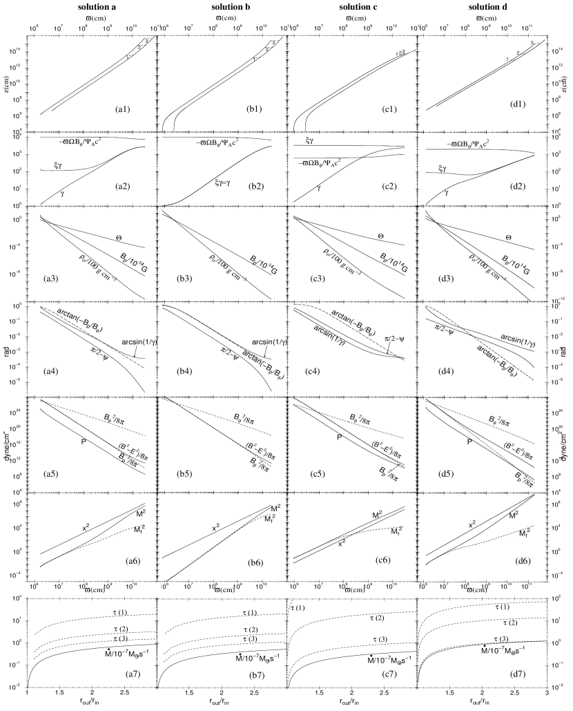
Figure 1: Main properties of the four representative solutions discussed in §4. See text for details.

Table 1: Parameters of Representative Solutions^†

solution	$F$	$x_{A}^{2}$	$\sigma_{M}$	$q$	$\mu$	$B_{0}\varpi_{0}^{2-F}$(cgs)	$\theta_{A}(\arcdeg)$	$\psi_{A}(\arcdeg)$	$p_{A}$	$\sigma_{A}$	$\varpi_{0}$($10^{6}$cm)
$a^{*}$	$1.01$	$0.99$	$5000$	$37.396$	$10116.1$	$1.35\times 10^{20}$	$35$	$72.7$	$-3.9\times 10^{-2}$	$86.6$	$2.5$
$b$	$1.01$	$0.9999$	$5000$	$0$	$9997.4$	$1.05\times 10^{20}$	$35$	$72.7$	$-5.0\times 10^{-4}$	$6820$	$2.5$
$c$	$1.01$	$0.15$	$300$	$322501$	$4053.2$	$5.93\times 10^{19}$	$35$	$72.0$	$-3.0$	$0.18$	$3$
$d$	$0.7$	$0.96$	$1000$	$44.92$	$2150$	$6.83\times 10^{21}$	$10$	$83.4$	$-0.93$	$23$	$2.5$
† In all cases $\Gamma=4/3\,,z_{c}=0$, and $r_{\rm out}/r_{\rm in}=3$.
∗ The solution presented in VK01 is the same as solution $a$, except that $B_{0}\varpi_{0}^{2-F}=2.96\times 10^{19}$ cgs and $\varpi_{0}=7.8125\times 10^{5}$ cm.

4.1 Solution $a$: A Hot, Fast-Rotator Outflow

This solution represents our fiducial model of a trans-Alfvénic GRB outflow in which the Poynting flux exceeds the enthalpy flux at the origin ($\mu\gg\xi_{i}$). The flow starts from the disk with a nonrelativistic velocity and in a short distance crosses the slow magnetosonic point (where $V_{p}\approx c/\sqrt{3}$). The acceleration in this regime is due to the pressure gradient force (the centrifugal acceleration is negligible for $\xi_{i}\gg 1$). The slow magnetosonic point arises from the interplay between the vertical gravitational and pressure-gradient forces. As we neglect gravity, we start the integration slightly above that slow point ($\gamma\gtrsim(3/2)^{1/2}$, see Fig. 1a2).

In this initial sub-Alfvénic regime, $M_{i}^{2}\ll 1-x_{A}^{2}\,,G_{i}^{2}\ll 1\,,x_{i}^{2}\ll x_{A}^{2}$. Equation (A2) for the Lorentz factor gives

$$\xi_{i}\gamma_{i}(1-x_{i}^{2})\approx\mu(1-x_{A}^{2})\,,\quad\mbox{or}\quad\xi_{i}\approx\mu(1-x_{A}^{2})\,.$$ (32)

Thus, a Poynting-dominated flow ($\mu\gg\xi_{i}$) is always close to being force-free ($x_{A}\approx 1$), and the initial enthalpy-to-Poynting flux ratio satisfies $\xi_{i}/\mu\approx 1-x_{A}^{2}$ ($=0.01$ in the displayed solution).

As the flow moves downstream it crosses the Alfvén singular point. We solve numerically for the slope $p_{A}$ of the Alfvénic Mach number that satisfies the Alfvén regularity condition (see §3.2.1).

In the super-Alfvénic regime there are three possible cases:
1. The flow recollimates ($\psi>\pi/2$) and there is a termination point where the entire energy is suddenly transformed into kinetic motion (corresponding to the solution hitting the modified fast singular surface but not being able to cross it);
2. The flow starts to decelerate at some heigh above the disk;
3. The flow becomes asymptotically cylindrical.

The last case is the only physically acceptable one and corresponds to a specific value of one of the model parameters. (For example, for the chosen parameter set $F$, $\theta_{A}$, $p_{A}$, $x_{A}$, $\sigma_{M}$, and $q$, there is a unique value of $\mu$ that corresponds to the cylindrical solution). This is the “magnetic nozzle” mechanism first described by Li et al. (1992) and discussed in §2.2.1. When the flow has cylindrical asymptotics, the asymptotic regime $\theta=0$ is the only possible solution of ${\cal D}=0$ (where ${\cal D}$ is given by eq. [26]). In this case, the modified fast-magnetosonic singular surface (the “event horizon” for the propagation of fast waves) corresponds to the asymptotic cylindrical regime (where all the fast Mach cones along each fieldline have the same opening angle). As in the “cold” solutions derived by Li et al. (1992), the critical value of $\mu$ is always close to $2\,\sigma_{M}$.

Figure 1a1 shows the meridional projections of the innermost and outermost fieldlines on a logarithmic scale. Our chosen initial cylindrical distances are $\varpi_{i}\approx 1.7\times 10^{6}$ cm for the innermost fieldline and $\approx 5.2\times 10^{6}$ cm for the outermost one; these distances are only slightly larger than those of the footpoints of these fieldlines in the disk. Figure 1a1 also depicts the optical paths of photons that originate at three points on the innermost fieldline; these were calculated according to the procedure described at the beginning of this section and are plotted as dashed lines labeled 1, 2, and 3. Figure 1a7 shows the corresponding optical depths $\tau(1)$, $\tau(2)$, and $\tau(3)$ along these paths as a function of $r_{\rm out}/r_{\rm in}=(\alpha_{\rm out}/\alpha_{\rm in})^{1/2}$. It is seen that, as one moves downstream (with the initial point on the innermost fieldline shifting to a larger height $z$ above the disk), the optical depth gets smaller, and the flow eventually becomes optically thin ($\tau(3)\approx 1$ for $r_{\rm out}/r_{\rm in}=3$).

Force densities in the meridional plane (a) along the poloidal flow and (b) in the transfield direction (toward the axis) for solution $a$.

Figure 1a7 also shows the radial profile of the mass-loss rate. For $r_{\rm out}/r_{\rm in}=3$, $\dot{M}\approx 10^{-7}\ M_{\sun}\ {\rm s}^{-1}$, corresponding to a total ejected baryonic mass of $M_{b}\approx 10^{-6}\,M_{\sun}$ for a typical burst duration $\Delta t\approx 10\,{\rm s}$.

The total energy flux along the poloidal flow is $\mu c^{2}\times\gamma\rho_{0}V_{p}$ (where $\gamma\rho_{0}V_{p}$ is the mass flux). The main part of the total energy flux (at least in the initial phase of the flow) is the Poynting flux (see eq. [2b]),

$$c\left(T^{0j}_{\rm EM}\hat{x}_{j}\right)\cdot\frac{{\boldsymbol{V}}_{p}}{V_{p}}=\frac{c}{4\pi}\left({\boldsymbol{E}}\times{\boldsymbol{B}}\right)\cdot\frac{{\boldsymbol{V}}_{p}}{V_{p}}=-\frac{\varpi\Omega B_{\phi}}{\Psi_{A}}\times\gamma\rho_{0}V_{p}\,.$$ (33)

(Note that this term is positive since $B_{\phi}<0$.) The remaining part $(\mu c^{2}+\varpi\Omega B_{\phi}/\Psi_{A})\times\gamma\rho_{0}V_{p}=\xi\gamma c^{2}\times\gamma\rho_{0}V_{p}$ (see the energy conservation relation, eq. [13d]) includes the kinetic energy flux ($\gamma\rho_{0}c^{2}(\gamma-1)V_{p}$) and the enthalpy flux. The total energy loss rate is $\dot{{\cal E}_{i}}=2\int\!\!\!\!\int\gamma\rho_{0}V_{p}\left(\xi\gamma c^{2}-\varpi\Omega B_{\phi}/\Psi_{A}\right)\frac{{\boldsymbol{V}}_{p}}{V_{p}}\cdot d{\boldsymbol{S}}=\mu\dot{M}c^{2}$, and for $\Delta t\approx 10$s the total energy injected into the two oppositely directed jets is ${\cal E}_{i}\approx 1.8\times 10^{52}\,{\rm ergs}$.

Figure 1a2 shows the various energy fluxes in units of $\gamma\rho_{0}c^{2}V_{p}$ (the mass flux $\times c^{2}$) as well as the Lorentz factor $\gamma$ as functions of $\varpi$, the distance from the axis of rotation along the innermost fieldline. We distinguish three different regimes:

1. Thermal acceleration region:
From the initial point (slightly above the slow point) up to $\sim 10^{8}$ cm, $\xi\gamma\approx\xi_{i}=const.$ (The exact initial values for solution $a$ are $\gamma_{i}=1.2$ and $\xi_{i}=114.8$.) The acceleration is primarily thermal: enthalpy is transformed into kinetic energy. In Figure 4.1a we see that the force $-{{\mathbf{f}}}_{G\parallel}$ (which measures the increase in $\gamma$) is equal to the temperature force ${{\mathbf{f}}}_{T\parallel}$ (which describes the decrease of $\xi$). The Poynting-to-mass flux ratio ($-\varpi\Omega B_{\phi}/\Psi_{A}$) is essentially constant, which means that the field is force-free; it only guides the flow. To a good approximation, $\gamma\approx\gamma_{i}\varpi/\varpi_{i}$ and $\xi\approx\xi_{i}\varpi_{i}/\varpi$. So long as $\xi\gg 1$, equation (29) gives $\xi\propto\Theta$; thus, $\Theta\approx\Theta_{i}\varpi_{i}/\varpi$. This is verified in Figure 1a3, which shows the poloidal magnetic field (in units of $10^{14}$ G) and the baryon rest-mass density (in units of $100$ g cm^-3). It is seen that $\rho_{0}\propto 1/\varpi^{3}$ (as expected from the polytropic relation $P\propto\rho_{0}^{4/3}$) and $B_{p}\propto 1/\varpi^{2}$ (as expected from the constancy of the mass-to-magnetic flux ratio $4\pi\gamma\rho_{0}V_{p}/B_{p}=\Psi_{A}$). As the azimuthal velocity is negligible (for a highly relativistic poloidal motion), equation (13a) implies $\varpi B_{\phi}=const.$, as expected in the force-free regime. In general, $V_{\phi}=cx+V_{p}B_{\phi}/B_{p}$, so $-B_{\phi}\approx xB_{p}=E$, consistent with $B_{p}\propto 1/\varpi^{2}$ and $B_{\phi}\propto 1/\varpi$.
Figure 1a4 shows the angle between the total magnetic field and its azimuthal component (which, given that $B_{p}\propto 1/\varpi^{2}$ and $-B_{\phi}\propto 1/\varpi$, decreases as $1/\varpi$), the “causal connection” opening angle $\arcsin(1/\gamma)\propto 1/\varpi$, and the opening half-angle of the outflow $\vartheta=\pi/2-\psi$ (its initial value is $\vartheta_{i}\approx 25\arcdeg$).
Figure 1a5 shows the pressures associated with the poloidal, azimuthal, and comoving magnetic field components, as well as the total thermal (lepton + radiation) pressure contribution ($B_{p}^{2}/8\pi\,,B_{\phi}^{2}/8\pi$ — dashed lines; $B_{\rm co}^{2}/8\pi=(B^{2}-E^{2})/8\pi\,,P$ — solid lines, respectively). In general, $B_{\rm co}^{2}\approx B_{p}^{2}+B_{\phi}^{2}/\gamma^{2}\approx B_{p}^{2}\left(1+x^{2}/\gamma^{2}\right)$. As $x$ and $\gamma$ are both proportional to $\varpi$, their ratio is a constant, $x/\gamma=x_{i}/\gamma_{i}\approx x_{i}\ll 1$. Thus, $B_{\rm co}\approx B_{p}$, as verified by the figure.
Figure 1a6 shows $x^{2}=\left(\varpi\Omega/c\right)^{2}$ and $M^{2}=\left(\gamma V_{p}\right)^{2}/\left(B_{p}^{2}/4\pi\rho_{0}\xi\right)$ (the squares of the “light cylinder” radius and the Alfvénic Mach number, respectively) as well as the square of the “classical fast-magnetosonic proper Mach number” $M_{f}^{2}\equiv\left(\gamma V_{p}\right)^{2}/U_{f}^{2}$, where $U_{f}$ is the larger solution of the quadratic

$$\left(\frac{U_{f}}{c}\right)^{4}-\left(\frac{U_{f}}{c}\right)^{2}\left(\frac{U_{s}^{2}}{c^{2}}+\frac{{B}^{2}-{E}^{2}}{4\pi\rho_{0}\xi c^{2}}\right)+\frac{U_{s}^{2}}{c^{2}}\frac{B_{p}^{2}\left(1-x^{2}\right)}{4\pi\rho_{0}\xi c^{2}}=0\,.$$ (34)

The point where $x=1$ corresponds to the light surface, which is close to the Alfvén surface $x=x_{A}$ (more accurately, the Alfvén surface is where $M^{2}=1-x_{A}^{2}$).
The point $M_{f}=1$ is the classical fast-magnetosonic point. It is seen that, up to that point, $M\approx M_{f}$. This can be understood by noting that, since $B^{2}-E^{2}\approx B_{p}^{2}\gg 4\pi\rho_{0}\xi U_{s}^{2}$, the solution of equation (34) yields $M^{2}/M_{f}^{2}=1/2+(1/4+x^{2}M^{2}U_{s}^{2}/\gamma^{2}V_{p}^{2})^{1/2}$. It follows that, so long as $x^{2}M^{2}U_{s}^{2}/\gamma^{2}V_{p}^{2}\leq x_{i}^{2}M^{2}/2\ll 1/2$ (using $U_{s}^{2}\leq c^{2}/2$), $M_{f}\approx M$.
At the classical fast point (subscript $f$) $M\approx 1\ll x$, so equation (A2) for the Lorentz factor gives $\gamma_{f}\approx\mu/\xi_{f}x_{f}^{2}$. If this point is located inside the thermally dominated region ($\xi_{f}\gg 1$, as in the depicted solution), then, using $\gamma_{f}\xi_{f}\approx\xi_{i}\gamma_{i}$, one infers $x_{f}\approx(\mu/\xi_{i}\gamma_{i})^{1/2}$. As $\gamma/x\approx\gamma_{i}/x_{i}$, it follows that $\gamma_{f}\approx(\mu\gamma_{i}/\xi_{i}x_{i}^{2})^{1/2}$.

2. Magnetic acceleration region:
From the end of the thermal acceleration zone, where $\xi\approx 1$, up to $\varpi\approx 10^{10}$ cm, it is seen from Figure 1a2 that the Lorentz factor continues to increase as $\gamma\propto\varpi^{\beta}$, with $\beta$ a constant $\approx 1$. This exponent is in general different for different solutions. We find that for solutions with a given $\mu$ but different $\xi_{i}$, $\beta$ is always less than 1 and decreases with increasing $\xi_{i}$. For larger $\xi_{i}$ the magnetic effects are less important, resulting in a weaker collimation of the flow and hence in a larger asymptotic width $\varpi_{\infty}$. Since the final Lorentz factor is $\sim\mu/2$, the exponent $\beta=d\ln\gamma/d\ln\varpi$ should be smaller. Centrifugal acceleration can also influence the magnitude of this exponent: for mildly relativistic flows we expect this acceleration to increase the lever arm of the flow, resulting in a lower value of $\beta$.
The acceleration in this region is due to magnetic effects: Poynting energy is transformed into kinetic energy. Figure 4.1a shows that the force $-{{\mathbf{f}}}_{G\parallel}$ (which describes the increase in $\gamma$) is equal to the Lorentz force ${{\mathbf{f}}}_{B\parallel}$ (which derives from the decrease of $\mid\varpi B_{\phi}\mid$). The Poynting-to-mass flux ratio declines from its initial value $\approx\mu c^{2}$ as $\mu c^{2}-\mid\varpi\Omega B_{\phi}/{\Psi_{A}}\mid\propto\varpi^{\beta}$, with $\beta\approx 1$, a result verified by Figure 1a2. However, the deviation from the initial value of $\mu c^{2}$ is not too strong, so the scalings $B_{p}\propto 1/\varpi^{2}$, $\rho_{0}\propto 1/\varpi^{3}$, and $-B_{p}/B_{\phi}\propto 1/\varpi$ remain approximately the same as at smaller radii (see Figs. 1a3, 1a4, and 1a5).
Figure 1a6 shows that $x\gg M$ but that $M$ increases faster than $x$. As the Poynting-to-matter energy flux ratio is $\left[c\left({\boldsymbol{E}}\times{\boldsymbol{B}}\right)\cdot{\hat{b}}/4\pi\right]/\left[\xi\gamma^{2}\rho_{0}c^{2}V_{p}\right]=(\mu-\xi\gamma)/\xi\gamma=(x^{2}-x_{A}^{2})/(M^{2}+1-x_{A}^{2})\approx x^{2}/M^{2}$, this is another manifestation of the Poynting-to-kinetic flux conversion.
The Bernoulli equation simplifies in this region to $\gamma\approx\gamma V_{p}/c$, which can be used, along with $\gamma\approx\mu M^{2}/\xi(x^{2}+M^{2})$ and equation (24c), to obtain the fieldline slope,

$$1-\frac{F\sigma_{M}}{\mu}\frac{x^{2}+M^{2}}{x^{2}}\approx 1-\frac{\sin(\theta-\vartheta)}{\sin\theta}\approx\frac{\vartheta}{\theta}=\left(\frac{d\ln\varpi}{d\ln z}\right)_{A=const}\ .$$ (35)

(The same result can be found using eq. [B2c].) So long as $x\gg M$, the slope is $1-F\sigma_{M}/\mu\approx 1/2$ (as the critical value for $\mu$ is close to $2\sigma_{M}$, and $F\approx 1$). Thus, the shape of the fieldlines is parabolic, $z\propto\varpi^{2}$, as Figure 1a1 verifies (cf. Contopoulos, 1995).

3. Asymptotic cylindrical region
At the end of the magnetic acceleration region the flow becomes cylindrical: Figure 1a1 shows that the fieldlines tend to a constant $\varpi$, whereas Figure 1a4 indicates that the opening half-angle $\vartheta=\pi/2-\psi$ tends to zero.
Figure 4.1b shows that, although the electric force almost cancels the magnetic force (${{\mathbf{f}}}_{B\bot}+{{\mathbf{f}}}_{E\bot}\ll{{\mathbf{f}}}_{B\bot}$), their sum ${{\mathbf{f}}}_{B\bot}+{{\mathbf{f}}}_{E\bot}\approx-{{\mathbf{f}}}_{C\bot}$. On the other hand, $-{{\mathbf{f}}}_{I\bot}\ll-{{\mathbf{f}}}_{C\bot}$, or (using eqs. [A8d] and [A8e]), $\varpi/{\cal R}\ll V_{\phi}^{2}\sin\psi/V_{p}^{2}$, which means that the poloidal curvature radius vanishes (i.e., the poloidal fieldlines become straight) — a characteristic of cylindrical collimation. (In the initial acceleration region near the disk it is seen from Fig. 4.1b that ${{\mathbf{f}}}_{B\bot}+{{\mathbf{f}}}_{E\bot}\approx-{{\mathbf{f}}}_{I\bot}$, which implies that the fieldlines curve toward the axis.)
In the cylindrical region, the transfield force-balance equation becomes

$$\rho_{0}\xi\gamma^{2}\frac{V_{\phi}^{2}}{\varpi}=\frac{d}{d\varpi}\left(P+\frac{B^{2}}{8\pi}\right)+\frac{B_{\phi}^{2}}{4\pi\varpi}-\frac{J^{0}}{c}E\,,$$ (36)

or, using $\alpha\propto\varpi^{2}$ and equations (24),

$$\rho_{0}\xi\gamma^{2}\frac{V_{\phi}^{2}}{\varpi}+2\frac{2-F}{\varpi}\left(P+\frac{B_{p}^{2}}{8\pi}\right)=\frac{F-1}{4\pi\varpi}\left(B_{\phi}^{2}-E^{2}\right)\,.$$ (37)

As the left-hand side of equation (37) is small but positive, $(F-1)\left(B_{\phi}^{2}-E^{2}\right)/B_{\phi}^{2}\approx 0^{+}$. Using $B_{\rm co}^{2}\approx B_{p}^{2}+B_{\phi}^{2}/\gamma^{2}$ and $B_{\rm co}^{2}=B_{p}^{2}+B_{\phi}^{2}-E^{2}$, we conclude that $B_{\phi}^{2}$ is invariably $\gtrsim E^{2}$; hence, only a current-carrying jet ($F>1$) can have cylindrical asymptotics.
Equation (35) with $d\varpi=0$ gives the final kinetic-to-Poynting flux ratio, $(M^{2}/x^{2})_{\infty}\approx(\mu/F\sigma_{M})-1\approx 1$, corresponding to $\gamma_{\infty}\approx\mu-F\sigma_{M}\approx\mu/2$. The value of $M^{2}$ becomes as large as that of $x^{2}$ (see Fig. 1a6), so a rough equipartition holds between the kinetic and Poynting fluxes: $\gamma_{\infty}\approx\left(-\varpi\Omega B_{\phi}/\Psi_{A}c^{2}\right)_{\infty}$ (see Fig. 1a2).
The implied conversion efficiency of $\sim 50\%$ between the total energy (injected largely in the form of a Poynting flux) and the final kinetic energy of the flow is consistent with the internal shock scenario for GRBs. Specifically, the asymptotic kinetic energy in each jet is $\sim 2\times 10^{51}\,{\rm ergs}$ for our fiducial parameters. With a radiative efficiency of $\gtrsim 10\%$ (e.g., Kobayashi, Piran, & Sari, 1997; Nakar & Piran, 2002b), this implies a radiated $\gamma$-ray energy of a few times $10^{50}$ ergs, as inferred observationally (Frail et al., 2001).
Figure 1a1 shows that, as the cylindrical region is approached, the Lorentz factor increases more slowly than $\propto\varpi$, resulting in a nonnegligible value of $x/\gamma$. Since $B_{\rm co}^{2}\approx B_{p}^{2}\left(1+x^{2}/\gamma^{2}\right)$, this explains the divergence of the $(B^{2}-E^{2})/8\pi$ and $B_{p}^{2}/8\pi$ curves in Fig. 1a5 near the cylindrical region. (Eq. [37] can be written as $(F-1)(B^{2}-E^{2})=B_{p}^{2}+4\pi\rho_{0}\xi\gamma^{2}V_{\phi}^{2}+8\pi(2-F)P$, which shows that $B^{2}-E^{2}\gtrsim B_{p}^{2}/(F-1)$ in the cylindrical regime.)
The condition that the GRB emission region be optically thin to the prompt $\gamma$-ray photons typically implies a lower limit $\gtrsim 100$ on the Lorentz factor of the outflow (e.g., Lithwick & Sari 2001). The asymptotic Lorentz factor attained in our fiducial solution (and, in fact, in the other three solutions presented in this section) readily satisfies this requirement.

4.1.1 Time-Dependent Effects

As noted at the beginning of §4, we approximate the outflow as a pair of pancakes that move in opposite directions away from the disk. In the context of the internal-shock scenario, each pancake consists of a number $N=100\ N_{2}$ of shells. The width of each shell is $\delta s=\Delta\ell/N=c\Delta t/N=3\times 10^{9}(\Delta t)_{1}/N_{2}$ cm, where the total duration of the burst is $\Delta t=10\ (\Delta t)_{1}$ s.

If the ejection of the shells from the disk surface ($\ell=0$) starts at time $t=0$ and ends at time $\Delta t$, then each shell can be labeled by its ejection time $t_{i}=s/c$, with $0\leq s\leq c\Delta t$. The shell “$s$” moves along the poloidal fieldline and at time $t$ its position is $\ell=\int_{s/c}^{t}V_{p}\ dt$. The distance between two neighboring shells $s$, $s+\delta s$ is (using $V_{p}\approx c-c/2\gamma^{2}$)

$$\delta\ell=\delta\left(\int_{s/c}^{t}V_{p}\ dt\right)\approx-\delta s+\displaystyle\int_{0}^{t}\frac{c}{\gamma^{2}}\frac{\delta\gamma}{\gamma}dt\,.$$ (38)

At early times the second term on the right-hand side of equation (38) is negligible and the frozen-pulse approximation holds (the distance between the two shells is constant, $\delta\ell\approx-\delta s$). However, even if the integrand in the second term is tiny, there will eventually come a time (call it $t_{c}$) when the integral will cancel the $-\delta s$ term (for $\delta\gamma/\delta s>0$, corresponding to the trailing shell moving faster than the leading one). One can integrate the equation of motion for each shell, $dz/dt=c(1-1/\gamma^{2})^{1/2}$, with $\gamma\approx\gamma_{i}\varpi/\varpi_{i}\approx\gamma_{i}(z/z_{i})^{1/2}$, to show that two neighboring shells with $\delta\gamma\sim\gamma$ will not collide for as long as they move in the flow acceleration zone. This is a reflection of the fact that the difference in the initial Lorentz factors of the two shells is not large enough to compensate for the longer acceleration time of the leading shell as it crosses this region, which also implies that the frozen-pulse assumption continues to hold throughout the acceleration zone. Only after the shells reach the constant-velocity, cylindrical-flow region, will the two shells collide ($\delta\ell=0$). Using equation (38), this will happen at a distance $\approx\gamma_{\infty}^{2}\delta s\approx 2\times 10^{16}(\Delta t)_{1}/N_{2}\ {\rm cm}$ beyond the end of the acceleration zone.

So long as the frozen-pulse approximation is valid, $\ell=\int_{s/c}^{t}V_{p}\ dt\approx ct-s$. As we proved in §2.1, it is possible to examine the motion of each shell in this regime using the $r$ self-similar model. If we focus on the shell $s_{0}$, then the parameter $F$ and boundary conditions $\{x_{A}(s_{0})\,,\,\mu(s_{0})\,,\,\sigma_{M}(s_{0})\,,\,q(s_{0})\,,\,B_{0}(s_{0})\varpi_{0}(s_{0})^{2-F}\}$ that we used to specify the solution refer to this particular $s_{0}$, and the corresponding solution $\{M(\theta,s_{0})\,,\,x(\theta,s_{0})\}$ is valid only for this shell.

In general, we may choose a different set $\{F\,,\,x_{A}(s)\,,\,\mu(s)\,,\,\sigma_{M}(s)\,,\,q(s)\,,\,B_{0}(s)\varpi_{0}(s)^{2-F}\}$ for a different shell $s$, but we have to be careful to also satisfy the assumption of a quasi-steady poloidal field, which requires all the shells to experience the same poloidal magnetic field at any given location. This requirement constrains the choice of boundary conditions.

No constraint is necessary in the force-free regime, in which the electromagnetic field is effectively decoupled from the matter in that there is no feedback from the matter acceleration to the field. The electromagnetic field only guides the flow and the motion is effectively HD. As we proved in VK01, one simply has to replace the spherical $r$ in the radial-outflow scalings (e.g., Piran, 1999) with the cylindrical radius $\varpi$ to get the correct scalings in the magnetically guided case.

However, in the superfast regime ($M^{2}\gg 1-x_{A}^{2}$, $x^{2}\gg x_{A}^{2}$), one finds that the (appropriately simplified) Bernoulli and transfield force-balance equations (eqs. [B2c] and [B2e]) become completely $s$-independent if one writes $M^{2}(\theta\,,s)={\cal M}^{2}(\theta)g(s)$, $x^{2}(\theta\,,s)={\cal X}^{2}(\theta)g(s)$, and $\mu(s)/\sigma_{M}(s)=\mu(s_{0})/\sigma_{M}(s_{0})$. ($F$ must also be $s$-independent.) Thus, we are free to specify the functions $g(s)$, $x_{A}(s)$, $\sigma_{M}(s)$, and $q(s)$ when $\mu(s)=\mu(s_{0})\sigma_{M}(s)/\sigma_{M}(s_{0})$, and from the fact that $A$ is $s$-independent we then also have $B_{0}(s)\varpi_{0}^{2-F}(s)x_{A}^{F}(s)/g^{F/2}(s)=B_{0}(s_{0})\varpi_{0}^{2-F}(s_{0})x_{A}^{F}(s_{0})/g^{F/2}(s_{0})$. These functions correspond to the initial conditions for each shell, obeying the quasi-steady poloidal magnetic field assumption.

Using $s=ct-\ell$ in any quantity $\Phi=\Phi(A\,,\ell\,,s)$, we may find either the time dependence following the motion of a particular shell: $\Phi=\Phi(A\,,ct-s\,,s)$ with $s$ held constant, or the time dependence at a given point in space as different shells pass by: $\Phi=\Phi(A\,,\ell\,,ct-\ell)$, with $\ell$ held fixed. The “initial” value $\Phi_{i}=\Phi(A\,,0\,,s)=\Phi(A\,,0\,,ct_{i})$ corresponds to the time $t=t_{i}=s/c$ when the shell $s$ is ejected from the surface $\ell=0$. Thus, we see that the $s$-dependence in $\Phi(A\,,\ell\,,s)$ represents the initial conditions at the ejection surface for each shell.

($a$) Baryon mass density plotted as a function of the arclength along the innermost fieldline of solution $a$ for several values of time since the start of the burst. The pancake width $(\Delta\ell)$ remains constant $\approx c\Delta t$. The dashed line represents the “time independent” solution for the reference shell $s_{0}=5\times 10^{10}$ cm, corresponding to the heavy dots. ($b$) Assumed form of the function $g(s)/\sigma_{M}(s)$ across the pancake. This function represents the initial baryon mass density in each shell ($\gamma\rho_{0i}(s)\propto g(s)/\sigma_{M}(s)$; see eq. [40]). The shell $s=0$, which is ejected first, has a tiny mass, the following shells have progressively larger masses, and the last shells ($s\lesssim c\Delta t$) again have negligible masses.

To illustrate how the time dependence in our model can be recovered, we now consider the baryon mass density along the flow. From equation (24d),

$$\gamma\rho_{0}(r\,,\theta\,,s)=\frac{\left[B_{0}(s_{0})\varpi_{0}^{2-F}(s_{0})\right]^{\frac{4}{F}}\mu(s_{0})x_{A}^{4}(s_{0})g(s)\ A^{2-\frac{4}{F}}}{4\pi c^{2}F^{\frac{4}{F}}\sigma_{M}(s_{0})g^{2}(s_{0})\left[{\cal M}^{2}(\theta)+{\cal X}^{2}(\theta)\right]\sigma_{M}(s)}$$

$$\times\frac{{\cal M}^{2}(\theta)g(s)-1+x_{A}^{2}(s)}{{\cal M}^{2}(\theta)g(s)}\frac{{\cal X}^{2}(\theta)g(s)+{\cal M}^{2}(\theta)g(s)}{{\cal X}^{2}(\theta)g(s)+{\cal M}^{2}(\theta)g(s)-1}\ .$$ (39)

Neglecting the second line (which is approximately equal to 1 in the non–force-free regime),

$$\gamma\rho_{0}(r\,,\theta\,,s)=\gamma\rho_{0}(r\,,\theta\,,s_{0})\frac{g(s)/\sigma_{M}(s)}{g(s_{0})/\sigma_{M}(s_{0})}\,.$$ (40)

Figure 4.1.1 shows $\gamma\rho_{0}$ as a function of the arclength along the inner fieldline at various times (as in the HD case illustrated in Fig. 1a of Piran et al. 1993). At each instant of time $t$, one can identify (using $s=ct-\ell$) which shell $s$ is at the point $\ell$. Knowing the distribution of $\gamma\rho_{0}$ as a function of $\ell$ for the reference shell $s_{0}$, one can obtain the density for all the other shells (corresponding to a particular choice of the function $g(s)/\sigma_{M}(s)$, such as the one depicted in Fig. 4.1.1b).

4.1.2 Validity of Assumptions

The ideal-MHD theory is not always a good approximation; in some cases it must be replaced by an exact multi-fluid theory including a relativistic Ohm’s law (e.g., Melatos & Melrose, 1996). A necessary condition for its applicability, derived from the need to attain the requisite charge density and current, implies a lower limit on the matter density (e.g., Spruit, Daigne, & Drenkhahn, 2001). The limits are $J\ll\rho_{0}q_{e}c/m_{p}$, $J^{0}/c\ll\rho_{0}q_{e}/m_{p}$ (where $q_{e}$ the electron charge), and we have verified that they are well satisfied in all of our solutions. In particular, the protons and the neutralizing electrons have a sufficiently large number density to screen the electric field parallel to the flow and to provide the necessary charge density and current.

Our neglect of gravity has turned out to be a valid approximation, since the flow near the disk is thermally dominated and the temperature force density near the origin of our fiducial solution (at $\varpi_{i}\approx 2\times 10^{6}\ {\rm cm}$, slightly above the slow-magnetosonic point) is ${{\mathbf{f}}}_{T\parallel}\approx 10^{19}$ dyne cm^-3, which is much larger than the gravitational force density associated with a central object of a few solar masses.

In § 4.1.1 we demonstrated that the frozen-pulse assumption is valid throughout the acceleration region.

We have also neglected the terms $\partial(E+B_{\phi})/\partial s$ and $\partial(E^{2}-B_{\phi}^{2})/\partial s$ in equation (2.1). Our results by and large verify these approximations, as we find that only near the asymptotic cylindrical region does $B_{\rm co}=(B_{p}^{2}+B_{\phi}^{2}-E^{2})^{1/2}$ deviate from $B_{p}$ (see Fig. 1a5). Even so, the ratio of the terms in equation (2.1) that contain $E+B_{\phi}$ over the last term in that equation is $\gamma(E+B_{\phi})/B_{\phi}$, which (using eq. [4]) becomes $\gamma(1-V_{p}/c)\ll 1$. An alternative argument supporting the conclusion that $E+B_{\phi}\approx 0$ is based on the requirements that $B_{\rm co}^{2}>0$ and $V_{\phi}>0$. The former gives (using $B_{\rm co}^{2}=B_{p}^{2}+B_{\phi}^{2}-E^{2}$ and eq. [12b]) $B_{\phi}^{2}/E^{2}>1-1/x^{2}$, whereas the latter yields (using eq. [9]) $B_{\phi}^{2}/E^{2}<c^{2}/V_{p}^{2}$. Thus, the ratio $B_{\phi}^{2}/E^{2}$ is bounded in a tiny interval around $1$, from $1-1/x^{2}$ to $c^{2}/V_{p}^{2}\approx 1+1/\gamma^{2}$.

4.2 Other Solutions

4.2.1 Solution $b$: The Cold Case ($\xi_{i}\approx 1$)

In the limit of low temperatures ($q\rightarrow 0$, $\xi\rightarrow 1$), we reproduce the exact cold relativistic solutions of Li et al. (1992), using a different parameter regime appropriate to GRB outflows. Contopoulos (1994) employed the same model but examined more massive flows that were not close to being force-free and thus were not accelerated as efficiently.

We present a cold solution in the second column of Figure 1; it can be readily compared with the fiducial solution $a$.

The cold solution is closer to being force-free, since $\gamma_{i}\approx 1/(1-x_{i}^{2})^{1/2}$ (using $V_{pi}\approx 0\,,V_{\phi i}\approx\varpi_{i}\Omega$), and hence (by eq. [32]) $\mu(1-x_{A}^{2})\approx(1-x_{i}^{2})^{1/2}\approx 1$. (For comparison, $\mu(1-x_{A}^{2})\approx\xi_{i}$ for solution $a$.)

Since the flow does not pass through a slow magnetosonic point in this case, we are able to find the solution all the way down to the disk surface. Near the origin the flow corotates with the disk ($V_{\phi}\approx cx$) and is accelerated due to the centrifugal force ${{\mathbf{f}}}_{C\parallel}$. The Lorentz factor does not increase linearly with $\varpi$ (but rather, to a good approximation, as $\gamma\approx 1/(1-x^{2})^{1/2}\approx(1+x^{2})^{1/2}$). However, the Lorentz force soon takes over and thereafter $\gamma\propto\varpi$ (see Fig. 1b2).

At the classical fast point $M_{f}\approx M\approx 1$, equation (A2) gives $\gamma_{f}\approx\mu/x_{f}^{2}$, which (using $\gamma_{f}\approx x_{f}$) can be transformed into the familiar form $\gamma_{f}\approx\mu^{1/3}$ (e.g., Camenzind, 1986). Unlike the purely monopole case (Michel, 1969), this point is located at a finite distance from the origin, and the bulk of the magnetic acceleration occurs further downstream.

The flow near the cylindrical regime is similar to that in the fiducial solution, as thermal effects are not important anymore. However, a signature of the cold solution can be seen in Figure 1b6 in the weaker deviation of $M$ from $M_{f}$. (The solution of eq. [34] in this case is $M_{f}^{2}/M^{2}=B_{p}^{2}/(B^{2}-E^{2})$, and the deviation of $M$ from $M_{f}$ is due only to $B^{2}-E^{2}$ becoming larger than $B_{p}^{2}$, which happens near the cylindrical region.)

4.2.2 Solution $c$: The Slow-Rotator Case ($\xi_{i}\approx\mu$)

This solution describes a slow rotator, in which the Poynting flux is smaller than the enthalpy flux (so $\mu\approx\xi_{i}$). The angular velocity of the inner fieldline is $\Omega=cx_{A}/\varpi_{0}=3873$ rad s^-1 (see Table 1), much smaller than the typical value ($\sim 10^{4}$ rad s^-1) near a solar-mass black hole. This solution is characterized by significantly higher $B_{p}/\mid B_{\phi}\mid$ ratios (see Fig. 1c4) and much lower values of $x$ (see Fig. 1c6) in comparison with solutions $a$ and $b$. It is also seen that this solution is not force-free: $x_{A}^{2}=0.15\ll 1$ (see eq. [32]). The acceleration in this case is thermal ($\xi\gamma\approx\mu$; see Fig. 1c2).

Nevertheless, since the flow is trans-Alfvénic, the poloidal magnetic pressure is much larger than the thermal pressure (see Fig. 1c5). This can be understood from the fact that, in general, one has at the Alfvén point

$$\left(\frac{B_{p}^{2}}{8\pi P}\right)_{A}=\left(\frac{2}{1-1/\xi}\frac{\left(\gamma V_{p}/c\right)^{2}}{1-x^{2}}\right)_{A}\approx\frac{2\gamma_{A}^{2}}{1-x_{A}^{2}}\gg 1\,.$$ (41)

Only when the flow is super-Alfvénic everywhere (even near the origin) can one obtain a hot, radial, HD-like solution with $P>B_{p}^{2}/8\pi$.

The magnetic field only guides the flow in this case. The collimation, however, is not very efficient (see Fig. 1c1). The flowlines “attempt” to become conical, but since in the framework of $r$ self-similarity the radial distance is given by $r=\varpi_{0}\alpha^{1/2}(A)G(\theta)/\sin\theta$, the only possible asymptotes as $r\rightarrow\infty$ are $\theta\rightarrow\theta_{\infty}$. For $\theta_{\infty}=0$ we have cylindrical asymptotics (as in solutions $a$ and $b$), and the only other possibility is for all the flowlines to have the same asymptotic opening half-angle, which is the situation depicted in Figure 1c1. This behavior can be understood if we write the transfield force-balance equation as

$$\frac{B_{p}^{2}}{4\pi{\cal R}}\left(M^{2}+x^{2}-1\right)=-\frac{1}{8\pi\varpi^{2}}\hat{n}\cdot{{{\mathbf{\nabla}}\!\!_{s}}}\left[\varpi^{2}\left(B_{\phi}^{2}-E^{2}\right)\right]+$$

$$+\frac{B_{p}^{2}}{4\pi\varpi}\left(\frac{MV_{\phi}}{V_{p}}\right)^{2}\hat{n}\cdot\hat{\varpi}-\hat{n}\cdot{\mathbf{\nabla}}\!\!_{s}\left(P+\frac{B_{p}^{2}}{8\pi}\right)$$ (42)

(see Vlahakis, 2003). By neglecting the centrifugal ($\propto V_{\phi}^{2}$) and the poloidal magnetic pressure terms and using equation (4) (which implies $E\approx-B_{\phi}V_{p}/c$), equation (4.2.2) can be rewritten as

$$\frac{B_{p}^{2}}{4\pi{\cal R}}\left(M^{2}+x^{2}-1\right)=-\frac{1}{8\pi\varpi^{2}}\hat{n}\cdot{\mathbf{\nabla}}\!\!_{s}\left(\frac{\varpi B_{\phi}}{\gamma}\right)^{2}-\hat{n}\cdot{\mathbf{\nabla}}\!\!_{s}P\,.$$ (43)

The first term on the right-hand side is positive and acts to collimate the flow (resulting in a positive poloidal curvature, ${\cal R}>0$), whereas the second term is negative and has the opposite effect on ${\cal R}$. In Poynting flux-dominated solutions, the pressure term is negligible and the collimation continues (albeit at a very low rate; see paper II) until the shape becomes cylindrical. However, when the thermal pressure becomes comparable to the comoving magnetic pressure (as in the present solution; see Fig. 1c5), the two terms on the right-hand side of equation (43) cancel each other. The curvature $1/{\cal R}$ thus vanishes before the cylindrical regime is reached, resulting in an asymptotic conical flow.

4.2.3 Solution $d$: The Return-Current Regime

For completeness, we also present a return-current ($J_{\parallel}>0$) solution. Since, near the disk surface, $-\varpi B_{\phi}\propto\alpha^{F-1}$ is a decreasing function of $\alpha$ in the $F<1$ case under consideration, the magnetic force acts to decollimate the flow (see § 2.2.2). This results in a weaker collimation than in the current-carrying ($F>1$) solutions (see Fig. 1d1). The electric force succeeds in collimating the flow despite the counter effect of the magnetic force; as discussed in §2.2.2, this is associated with the positive charge density ($J^{0}>0$) expected in the return-current regime. Examining the forces in the transfield direction, we find that ${{\mathbf{f}}}_{E\bot}\gg{{\mathbf{f}}}_{E\bot}+{{\mathbf{f}}}_{B\bot}\approx-{{\mathbf{f}}}_{I\bot}\gg-{{\mathbf{f}}}_{C\bot}$; i.e., the Lorentz force is balanced by the inertial force. (This can be contrasted with the cylindrical solution $a$, where the balance is provided by the centrifugal force: ${{\mathbf{f}}}_{B\bot}\gg{{\mathbf{f}}}_{E\bot}+{{\mathbf{f}}}_{B\bot}\approx-{{\mathbf{f}}}_{C\bot}\gg-{{\mathbf{f}}}_{I\bot}$; see Figure 4.1b). As in the nonrelativistic, cold MHD flow considered by Blandford & Payne (1982), the curvature radius is nonnegligible and the solution terminates at a finite height above the disk.

5 Discussion and Conclusion

We regard the fiducial solution $a$ as providing the most plausible representation of an accelerating GRB outflow. Neutrino energy deposition and magnetic field dissipation are likely to give rise to a nonnegligible thermal component at the origin, as envisioned in the original fireball scenario. Such a component is incorporated into solution $a$ but is missing in solution $b$. It is, nevertheless, worth reemphasizing that the dominant energy source even in solution $a$ is the Poynting flux. We note in this connection that one of the potential problems of traditional fireball models has been the “baryon contamination” issue: Why does the highly super-Eddington luminosity that drives the fireball not lead to a more significant mass loading of the flow and thereby keep $\gamma_{\infty}$ comparatively low? If most of the requisite energy were injected in a nonradiative form, then this problem would be alleviated. The expectation that GRB outflows are Poynting flux-dominated also renders the slow-rotator (enthalpy flux-dominated) solution $c$ less relevant to their interpretation than the fiducial solution.

GRB outflows are inferred to be highly collimated at large distances from the origin: this has motivated us to construct our fiducial solution in the current-carrying ($J_{\parallel}<0$) regime, which is applicable near the symmetry axis (see Fig. 2.2.2). However, as demonstrated in Figure 1, the illustrative current-carrying solution $d$ also becomes well collimated on a similar length scale, so it may also provide an adequate representation of such outflows. In fact, this regime may be a natural choice for modeling the far-downstream region of the flow since it corresponds to a plausible current-configuration on large scales; furthermore, as shown in Vlahakis (2003), it also results in a more efficient acceleration. We have opted to focus on the current-carrying regime in this paper since the solutions in this case, unlike the return-current solutions formally extends to infinity. We incorporate the return-current regime into a GRB outflow model in Vlahakis at al. (2003).

Our fiducial self-similar “hot” solution as well as our “cold” relativistic MHD solution (and the corresponding ones derived by Li et al. 1992 and Contopoulos 1994) have cylindrical asymptotics. In the nonrelativistic theory, it was shown (Vlahakis & Tsinganos, 1998) that it is possible to derive exact solutions of radially self-similar flows that have either one of the following three types of asymptotes: cylindrical, parabolic, or conical. Although we expect that it should be possible to obtain different asymptotic behaviors also in radially self-similar relativistic flows, this has not yet been studied in detail. Our basic conclusions about the magnetic acceleration of the flow do not, however, depend on the shape of the asymptotic flowlines, although the quantitative constraints on the mass loading (to assure that the flow is optically thin in the shell-collision region) would be eased if the flow continued to expand rather than collimated to a cylinder. GRB jets are often modeled in terms of conical jets, and this picture has gained support from observations of a panchromatic break in the light curve of several GRB afterglows (from which jet half-opening angles in the range of $2^{\circ}$ to $20^{\circ}$ have been inferred; e.g., Panaitescu & Kumar 2002). However, a sharp physical boundary may not be required for interpreting the data in the context of a beam-patterned outflow (e.g., Rossi, Lazzatti, & Rees, 2002; Lyutikov & Blandford, 2002). Furthermore, it has been argued that a cylindrical jet model could provide a better fit to the light curves of at least some afterglows and might perhaps even be able to account for the panchromatic breaks commonly attributed to a finite jet opening angle (e.g., Dar, 1998; Cheng, Huang, & Lu, 2001).

Even if GRB jets are not characterized by a global cylindrical geometry, the asymptotically cylindrical solutions that we derived may be applicable to the “patchy shell” scenario for variable GRB outflows (Kumar & Piran, 2000). In this picture, the outflowing shells are ejected within a given opening angle but do not fill the entire solid angle into which they are injected. In the context of the internal shock model, this scenario alleviates the energy requirements on bright bursts; it is also consistent with the apparent lack of a strong correlation between the prompt high-energy and the afterglow fluences, and it may account for the early-time variability in the afterglow emission of a source like GRB 021004 (Nakar, Piran, & Granot, 2003). In the phenomenological model considered by Kumar & Piran (2000), successive blobs of angular scale $1/\gamma_{\infty}$ are ejected randomly within an opening angle of $10^{\circ}$, and the number of blobs ejected along a given direction (given that more than one is required for the production of internal shocks) is also taken to be a random number (distributed uniformly in a predetermined range). This model was intended to mimic the behavior of causally disconnected regions in large-scale ejected shells. An alternative physical picture is that of a collection of magnetically active regions on the surface of the disk that feed the GRB outflow. In this picture, the magnetic field associated with each “patch” guides successive “mini” shells along roughly congruent paths, thereby enhancing the efficiency of internal-shock production. However, the ejection directions from different sites need not be parallel to each other, so some of the beamed $\gamma$-ray emission may miss the observer: this might contribute to the appearance of quiescent times between GRB pulses (Nakar & Piran, 2002a).

The high ($\sim 50\%$) Poynting-to-kinetic energy conversion efficiency exhibited by all our fast-rotator solutions (solutions $a$, $b$, and $d$) has made it possible for our models to accommodate the internal-shock emission scenario without requiring a prohibitively large energy input at the source (see §4). However, currently available data on the radiated $\gamma$-ray energy $E_{\gamma}$ (e.g., Panaitescu & Kumar, 2002) and the outflow kinetic energy $E_{K}$ (e.g., Frail et al., 2001), which indicate that they are both approximately equal ($\sim 10^{51}\,{\rm ergs}$), are inconsistent with this scenario for any reasonable radiative energy efficiency of such shocks (see Nakar & Piran 2002b for further discussion of this issue). One possible resolution of this apparent inconsistency is that the prompt high-energy emission arises directly from electromagnetic energy dissipation without the intermediate step of Poynting-to-bulk-kinetic energy conversion (e.g., Thompson, 1994; Smolsky & Usov, 2000; Lyutikov & Blackman, 2001; Drenkhahn & Spruit, 2002). Our solutions seem to be consistent with this possibility: they imply that about half of the injected energy is converted into bulk kinetic energy; if the remaining Poynting flux can be efficiently converted into high-energy emission, then this would lead to an approximate equality between $E_{\gamma}$ and $E_{K}$. Drenkhahn & Spruit (2002) used ideal-MHD equations with parameterized magnetic energy dissipation to demonstrate (in the context of a strictly radial flow, i.e., without taking into account the transfield force-balance equation that determines the fieldline shape) that the Poynting-to-radiation energy conversion could in principle be as high as 50% and that the dissipation may also result in significant bulk acceleration. It would be interesting to combine the approach taken by these authors (see also Spruit et al. 2001 and Drenkhahn 2002) with the one utilized in this paper to consider the effects of dissipation in a nonradial flow.

We now briefly compare the results of our exact solutions with some of the previous work on MHD effects in GRB outflows. The incorporation of “disposable” magnetic energy into the traditional fireball model was discussed by Mészáros et al. (1993). The behavior that they infer is consistent with our solutions in the regime where $\gamma\propto\varpi$ (but not beyond it). Usov (1994) interpreted the outflows in terms of pulsar winds that generate intense electromagnetic waves at the point where the ideal-MHD approximation breaks down. He highlighted the fact that the Lorentz factors of the particles accelerated by such waves could be as high as $\sim\mu^{2/3}$ and thus greatly exceed the terminal Lorentz factors ($\sim\mu^{1/3}$) attained in the Michel (1969) ideal-MHD monopole solution. The acceleration efficiency of our collimating (and thus nonmonopolar) ideal-MHD solutions is much higher yet: they yield $\gamma_{\infty}\approx\mu/2\gg\mu^{2/3}$.

Mészáros & Rees (1997) examined a magnetized conical jet with a pure electron-positron composition. They deduced (and our solutions have confirmed) that the pair–photon fluid is initially accelerated by thermal pressure, with the magnetic field acting only to guide the flow. They also pointed out that radiation drag effects allow the pairs and photons to remain coupled even beyond the point where the scattering optical depth drops below 1 and that at some point pair annihilation freezes out. Grimsrud & Wasserman (1998) subsequently showed that the surviving pairs carry only a fraction $\sim 10^{-5}\gamma_{i}^{3/4}$ of the initial energy, implying that, in the absence of magnetic acceleration, this scenario is extremely inefficient. We note, however, that if a nonnegligible fraction ($1-\gamma_{i}\xi_{i}/\mu$) of the total injected energy is in magnetic form ([with the ratio of magnetic to pairs-plus-photons energy injection rates being $(\mu-\gamma_{i}\xi_{i})/\gamma_{i}\xi_{i}\approx\gamma_{i}$, as assumed by Mészáros & Rees 1997), then, based on our “cold” solution (see § 4.2.1), half of the magnetic energy could be eventually transformed into kinetic energy of the surviving pairs, reaching overall efficiencies $\sim(\mu-\xi_{i}\gamma_{i})/2\mu$. For $\gamma_{i}\sim 1$ this yields an efficiency of $\sim 25\%$, which is significantly higher than the values estimated by Mészáros & Rees (1997). As was, however, discussed by these authors, the resulting outflow would have a huge Lorentz factor and might not by itself be able to reproduce the observed properties of real GRBs.

Although the presentation in this paper and its companion is focused on the application to GRBs, our formalism is quite general and the solutions that we present should be relevant also to other magnetically driven relativistic outflow sources, notably AGNs and microquasars. The possible relationship between the different classes of beamed relativistic outflows in astrophysics has already been noted before by various authors. One potential attraction of adopting a common modeling framework for these outflows is that it could shed new light on each of the different types of sources. For example, the concept of internal shocks was originally proposed in the context of AGN jets (Rees, 1978), and it has recently been adopted also for modeling microquasars (Kaiser, Sunyaev, & Spruit, 2000). In the latter class of objects, there is direct observational evidence (in the form of correlated X-ray, infrared, and radio flux variations and the appearance of superluminal radio knots) for a causal connection between a rapid accretion episode onto the central black hole and the ejection of superluminal blobs (e.g., Mirabel & Rodríguez, 1999). This is the same basic scenario as the one commonly adopted (albeit without direct observational support) for GRB outflows. A similar correlation between the X-ray and radio flux behavior and the appearance of radio-bright superluminal knots was recently discovered also in an AGN jet (Marscher et al., 2002). Although the observed behavior in this case does not support the notion that AGNs are a simple scaled-up version of microquasars, this might be attributable to a different origin of the underlying disk instability that induces the accretion/ejection episodes (e.g., Menou & Quataert, 2001) or to different environmental conditions (e.g., Heinz, 2002).

There is now also evidence that the high-energy (GeV-range) $\gamma$-ray emission in the blazar class of AGNs originates in superluminal radio knots — which likely represent discrete blobs or shocks in a relativistic jet — at a large distance from the origin (e.g., Jorstad et al., 2001b). This is essentially the picture envisioned for GRB outflows. The superluminal knots in blazar jets such as 3C 345 (e.g., Unwin et al., 1997) and 3C 279 (e.g., Wehrle et al., 2001) are inferred to move along distinct curved paths, although in the former case it has been argued (Wardle et al., 1996) that at least two of the knots follow each other along the same trajectory. This behavior is consistent with the “patchy shell” model discussed above in connection with GRBs. There are also indications that the outflows continue to accelerate on large scales: for example, the Lorentz factor of knot C7 in the quasar 3C 345 was inferred to increase from $\sim 3$ to $\gtrsim 10$ as it moved from a distance of $r\simeq 3\,{\rm pc}$ from the galactic nucleus to $r\simeq 20\,{\rm pc}$ (Unwin et al., 1997). A scaled-down version of this behavior was found in the radio galaxy NGC 6251, where knots in the radio jets were inferred to accelerate from $\sim 0.13\,c$ at $r\approx 0.53\,{\rm pc}$ to $\sim 0.42\,c$ at $r\approx 1.0\,{\rm pc}$ (Sudou et al., 2000). Such large-scale acceleration is most naturally interpreted in terms of a Poynting-dominated jet model of the type discussed in this paper (N. Vlahakis & A. Königl, in preparation).

In conclusion, we have derived in this paper the general formalism for radially self-similar, relativistic MHD outflows and presented exact solutions (obtained by solving the Euler and transfield equations and imposing regularity conditions at the relevant critical points) to illustrate their basic properties. We focused on trans-Alfvénic flows, deferring a discussion of super-Alfvénic solutions to the companion paper. We considered “hot” and “cold” rapid-rotator flows (the latter reproducing previous results by Li et al. 1992 and Contopoulos 1994) as well as slow-rotator flows in the current-carrying regime (which should apply near the rotation axis), but also described a “hot,” fast-rotator solution in the return-current regime. In all cases, we demonstrated that the Poynting flux injected at the source can be transformed with high ($\sim 50\%$) efficiency into kinetic energy of relativistic baryons at a large (but finite) distance from the origin. We concentrated on applications to GRB outflows, although we pointed out that similar solutions may describe jet acceleration in AGNs and microquasars. In the application to GRBs, we presented a particular “hot,” fast-rotator outflow as a fiducial solution. In this case the outflow is initially accelerated thermally, with the magnetic field acting only to guide and collimate it, but subsequently magnetic effects become fully dominant and are responsible for the bulk of the acceleration (which occurs between the classical fast-magnetosonic and modified fast-magnetosonic surfaces) and for the final collimation to cylindrical asymptotics. We stress, however, that this solution is only illustrative and is not meant to provide an accurate description of a typical GRB flow. As we discuss in Paper II, super-Alfvénic outflows can also provide plausible representations of GRB outflows; their basic properties, however, are quite similar to those of trans-Alfvénic flows. We have, furthermore, concluded that solutions in the return-current regime may also be relevant to these flows; we address this possibility in greater detail in a separate publication (Vlahakis at al., 2003).

Appendix A Equations in the Axisymmetric Case with E${}_{\phi}=0$

We may combine equations (13a), (13c), and (13d) to obtain $\gamma\,,V_{\phi}$, and $B_{\phi}$ as functions of $M\,,$ $x$, and $G$ using

$${\boldsymbol{B}}=\frac{{\mathbf{\nabla}}\!\!_{s}A\times\hat{\phi}}{\varpi}-\frac{\mu c\Psi_{A}x_{A}^{2}}{x}\frac{1-G^{2}}{1-M^{2}-x^{2}}\hat{\phi}\,,\quad{\boldsymbol{E}}=-\frac{\Omega}{c}{\mathbf{\nabla}}\!\!_{s}A\,,$$ (A1)

$${\boldsymbol{V}}=\frac{\Psi_{A}}{4\pi\gamma\rho_{0}}{\boldsymbol{B}}+\varpi\Omega\hat{\phi}=\frac{\Psi_{A}}{4\pi\gamma\rho_{0}}\frac{{\mathbf{\nabla}}\!\!_{s}A\times\hat{\phi}}{\varpi}+\frac{\varpi_{A}\Omega}{G}\frac{G^{2}-M^{2}-x^{2}}{1-M^{2}-x_{A}^{2}}\hat{\phi}\,,\quad\gamma=\frac{\mu}{\xi}\frac{1-M^{2}-x_{A}^{2}}{1-M^{2}-x^{2}}\,,$$ (A2)

$$\rho_{0}=\frac{\xi\Psi_{A}^{2}}{4\pi M^{2}}\,,\quad P=Q\rho_{0}^{\Gamma}\,,\quad\xi=1+\left(\int_{0}^{P}\frac{dP}{\rho_{0}c^{2}}\right)_{\{s\,,\ A\,=\,const\}}=1+\frac{\Gamma}{\Gamma-1}\frac{P}{\rho_{0}c^{2}}\,.$$ (A3)

Knowing the field-line constants (for each $s$)

$$\varpi_{A}(A\,,s)\equiv\left(\frac{L}{\mu\Omega}\right)^{1/2}\,,\quad x_{A}(A\,,s)\equiv\frac{\varpi_{A}\Omega}{c}\,,\quad\mu(A\,,s)\,,\quad\sigma_{M}(A\,,s)\equiv\frac{A\Omega^{2}}{c^{3}\Psi_{A}}\,,\quad q(A\,,s)\equiv\frac{\Psi_{A}^{2}}{4\pi}\left(\frac{\Gamma}{\Gamma-1}\frac{Q}{c^{2}}\right)^{\frac{1}{\Gamma-1}}\,,$$ (A4)

we can find the quantities $x\,,M\,,G\,,\xi$ (which in general are functions of $A\,,\ell$, and $s$) by solving the following system of equations:

$$x=x_{A}G\,,\quad M^{2}=q\frac{\xi}{\left(\xi-1\right)^{\frac{1}{\Gamma-1}}}\ ,$$ (A5)

the Bernoulli equation

$$\frac{\mu^{2}}{\xi^{2}}\frac{G^{2}(1-M^{2}-x_{A}^{2})^{2}-x_{A}^{2}(G^{2}-M^{2}-x^{2})^{2}}{G^{2}(1-M^{2}-x^{2})^{2}}=1+\frac{\sigma_{M}^{2}}{\xi^{2}}\frac{M^{4}}{x^{4}}\left(\frac{\varpi{\mathbf{\nabla}}\!\!_{s}A}{A}\right)^{2}\ ,$$ (A6)

which is obtained after substituting all quantities in the identity $\gamma^{2}\left(1-{V_{\phi}^{2}}/{c^{2}}\right)=1+\gamma^{2}{V_{p}^{2}}/{c^{2}}$ using equations (A1,A2) and which in the nonrelativistic limit takes the familiar form (after Taylor expanding in $1/c^{2}$)

$${\frac{V^{2}}{2}+\frac{\Gamma}{\Gamma-1}\frac{P}{\rho_{0}}-\frac{\varpi\Omega B_{\phi}}{\Psi_{A}}=(\mu-1)c^{2}}\,,$$

and the transfield equation (obtained from the component of the momentum equation along $-{\boldsymbol{\nabla}}A$)

$$\left[x^{2}\left({\mathbf{\nabla}}\!\!_{s}A\right)^{2}\frac{\partial\ln\left(\displaystyle\frac{x_{A}(A\,,s)}{\varpi_{A}(A\,,s)}\right)}{\partial A}-\L A(1-M^{2}-x^{2})\right]\left(\frac{{\mathbf{\nabla}}\!\!_{s}A}{\varpi}\right)^{2}+$$

$$+\left[\frac{2x_{A}^{2}}{\varpi_{A}^{3}G}\left({\mathbf{\nabla}}\!\!_{s}A\right)^{2}+\frac{\mu^{2}x_{A}^{6}A^{2}}{\varpi_{A}^{5}\sigma_{M}^{2}M^{2}G^{3}}\left(\frac{G^{2}-M^{2}-x^{2}}{1-M^{2}-x^{2}}\right)^{2}\right]\hat{\varpi}\cdot{\mathbf{\nabla}}\!\!_{s}A-$$

$$-\frac{M^{2}}{2}{\mathbf{\nabla}}\!\!_{s}\left[\left(\frac{{\mathbf{\nabla}}\!\!_{s}A}{\varpi}\right)^{2}\right]\cdot{\mathbf{\nabla}}\!\!_{s}A-\frac{\Gamma-1}{\Gamma}{\mathbf{\nabla}}\!\!_{s}\left[\frac{\xi(\xi-1)}{M^{2}}\frac{A^{2}x_{A}^{4}}{\sigma_{M}^{2}\varpi_{A}^{4}}\right]\cdot{\mathbf{\nabla}}\!\!_{s}A-$$

$$-\frac{1}{2\varpi^{2}}{\mathbf{\nabla}}\!\!_{s}\left[\frac{\mu^{2}A^{2}x_{A}^{6}}{\sigma_{M}^{2}\varpi_{A}^{2}}\left(\frac{1-G^{2}}{1-M^{2}-x^{2}}\right)^{2}\right]\cdot{\mathbf{\nabla}}\!\!_{s}A=0\,,$$ (A7)

where the operator $\L\equiv{\boldsymbol{\nabla}}^{2}-(2/\varpi){\hat{\varpi}}\cdot{\boldsymbol{\nabla}}$ is related to the curvature radius ${\cal R}=\mid{\boldsymbol{\nabla}}A\mid\left(\L A-{\boldsymbol{\nabla}}A\cdot{\boldsymbol{\nabla}}\ln\mid{\boldsymbol{\nabla}}A/\varpi\mid\right)^{-1}$.

The latter equation can be written as

$${{\mathbf{f}}}_{G\bot}+{{\mathbf{f}}}_{T\bot}+{{\mathbf{f}}}_{C\bot}+{{\mathbf{f}}}_{I\bot}+{{\mathbf{f}}}_{P\bot}+{{\mathbf{f}}}_{E\bot}+{{\mathbf{f}}}_{B\bot}=0\,,$$ (A8a)

where the subscript $$\bot \hat{n}=\hat{b}\times\hat{\phi}=-{\boldsymbol{\nabla}}A/\mid{\boldsymbol{\nabla}}A\mid$$ denotes the component of a force perpendicular to the poloidal fieldline and pointing toward the axis (along ), and where the individual terms are given by

$${{\mathbf{f}}}_{G\bot}=0\,,$$ (A8b)

$${{\mathbf{f}}}_{T\bot}=0\,,$$ (A8c)

$${{\mathbf{f}}}_{C\bot}=-\frac{\gamma^{2}\rho_{0}\xi V_{\phi}^{2}}{\varpi}\sin\psi=-\frac{B_{0}^{2}}{4\pi\varpi_{0}}\frac{c^{2}\Psi_{A}^{2}}{B_{0}^{2}}\frac{x_{A}^{2}\mu^{2}}{\alpha^{1/2}}\frac{1}{M^{2}G^{3}}\left(\frac{G^{2}-M^{2}-x^{2}}{1-M^{2}-x^{2}}\right)^{2}\frac{\hat{\varpi}\cdot{\mathbf{\nabla}}\!\!_{s}\alpha}{\mid{\mathbf{\nabla}}\!\!_{s}\alpha\mid}\ ,$$ (A8d)

$${{\mathbf{f}}}_{I\bot}=-\frac{\gamma^{2}\rho_{0}\xi V_{p}^{2}}{{\cal R}}=-\frac{M^{2}B_{p}^{2}}{4\pi{\cal R}}=\frac{B_{0}^{2}}{4\pi\varpi_{0}}\left\{\frac{M^{2}\varpi_{0}^{5}}{8}{\mathbf{\nabla}}\!\!_{s}\left[\left(\frac{{\mathbf{\nabla}}\!\!_{s}{\cal A}}{\varpi}\right)^{2}\right]\cdot\frac{{\mathbf{\nabla}}\!\!_{s}\alpha}{\mid{\mathbf{\nabla}}\!\!_{s}\alpha\mid}-\frac{M^{2}\varpi_{0}^{3}\mid{\mathbf{\nabla}}\!\!_{s}{\cal A}\mid}{4\alpha G^{2}}\L{\cal A}\right\}\ ,$$ (A8e)

$${{\mathbf{f}}}_{P\bot}=\frac{B_{0}^{2}}{4\pi\varpi_{0}}\frac{\Gamma-1}{\Gamma}\varpi_{0}{\mathbf{\nabla}}\!\!_{s}\left[\frac{\xi(\xi-1)}{M^{2}}\frac{c^{2}\Psi_{A}^{2}}{B_{0}^{2}}\right]\cdot\frac{{\mathbf{\nabla}}\!\!_{s}\alpha}{\mid{\mathbf{\nabla}}\!\!_{s}\alpha\mid}\ ,$$ (A8f)

$${{\mathbf{f}}}_{E\bot}=-\frac{B_{0}^{2}}{4\pi\varpi_{0}}\frac{x_{A}^{2}\varpi_{0}\mid{\mathbf{\nabla}}\!\!_{s}{\cal A}\mid}{4\alpha}\left[\varpi_{0}^{2}\L{\cal A}+\frac{2}{G\alpha^{1/2}}\varpi_{0}\hat{\varpi}\cdot{\mathbf{\nabla}}\!\!_{s}{\cal A}+\left(\varpi_{0}{\mathbf{\nabla}}\!\!_{s}{\cal A}\right)^{2}\left(\frac{1}{x_{A}}\frac{dx_{A}}{{\cal A}}-\frac{1}{2\alpha}\frac{d\alpha}{d{\cal A}}\right)\right]\ ,$$ (A8g)

$${{\mathbf{f}}}_{B\bot}=\frac{B_{0}^{2}}{4\pi\varpi_{0}}\left\{\frac{1}{2\alpha G^{2}}\varpi_{0}{\mathbf{\nabla}}\!\!_{s}\left[\alpha x_{A}^{2}\mu^{2}\frac{c^{2}\Psi_{A}^{2}}{B_{0}^{2}}\left(\frac{1-G^{2}}{1-M^{2}-x^{2}}\right)^{2}\right]\cdot\frac{{\mathbf{\nabla}}\!\!_{s}\alpha}{\mid{\mathbf{\nabla}}\!\!_{s}\alpha\mid}+\frac{\varpi_{0}\mid{\mathbf{\nabla}}\!\!_{s}{\cal A}\mid}{4\alpha G^{2}}\varpi_{0}^{2}\L{\cal A}\right\}\ .$$ (A8h)

Appendix B Equations in the $r$ Self-Similar Case

In the $r$ self-similar model described in §3, the integrals of motion have the following form:

$$\sigma_{M}=\sigma_{0}\left[1-\left(\frac{\alpha_{0}}{\alpha}\right)^{\frac{F}{2}}\right]\,,\quad\mbox{where}\quad\sigma_{0}\,,\alpha_{0}=const\,,\quad\mu\,,x_{A}\,,q=const\,,\quad A=\frac{B_{0}\varpi_{0}^{2}}{F}\left(\alpha^{\frac{F}{2}}-\alpha^{\frac{F}{2}}_{0}\right)\ ,$$ (B1a)

with the fieldline constants given by

$$\Psi_{A}=\frac{B_{0}x_{A}^{2}}{F\sigma_{0}c}\alpha^{\frac{F-2}{2}}\,,\quad\Omega=\frac{x_{A}c}{\varpi_{0}\alpha^{1/2}}\,,\quad L=c\varpi_{0}x_{A}\mu\alpha^{1/2}\,,\quad Q=c^{2}\frac{\Gamma-1}{\Gamma}\left(\frac{4\pi c^{2}F^{2}\sigma_{M}^{2}q}{x_{A}^{4}B_{0}^{2}\alpha^{F-2}}\right)^{\Gamma-1}\,.$$ (B1b)

Note that $$\sigma_{M}$$ is the “magnetization parameter” in the monopole solution of Michel (1969).

In cases where $F>0$, the requirement that the magnetic flux function $A$ vanishes on the rotation axis $\alpha=0$ implies that $\alpha_{0}=0$ when $\sigma_{M}=const$ and $A=\frac{B_{0}\varpi_{0}^{2}}{F}\alpha^{\frac{F}{2}}$. We examine solutions with $\alpha_{0}=0$ throughout this paper.

Equations (A5) and (A6) take the form

$$x=x_{A}G\,,$$ (B2a)

$$M^{2}=q\frac{\xi}{\left(\xi-1\right)^{\frac{1}{\Gamma-1}}}\ ,$$ (B2b)

$$\frac{\mu^{2}}{\xi^{2}}\frac{G^{4}\left(1-M^{2}-x_{A}^{2}\right)^{2}-x^{2}\left(G^{2}-M^{2}-x^{2}\right)^{2}}{G^{4}\left(1-M^{2}-x^{2}\right)^{2}}=1+\frac{F^{2}\sigma_{M}^{2}M^{4}\sin^{2}\theta}{\xi^{2}x^{4}\cos^{2}\left(\psi+\theta\right)}\ ,$$ (B2c)

and can be solved for $$x\,,\xi \psi$$, and .

Using $\ \tan\psi=\left(\partial z/\partial\varpi\right)_{A}$ and equation (17), we get $\ \tan\psi=d(G/\tan\theta)/dG\,,$ or,

$$\frac{dG^{2}}{d\theta}=\frac{2G^{2}\cos\psi}{\sin\theta\,\cos\left(\psi+\theta\right)}\ .$$ (B2d)

The transfield equation (A) becomes

$$G\sin^{2}\theta\frac{d}{d\theta}\left[\tan\left(\psi+\theta\right)\frac{1-M^{2}-x^{2}}{G}\right]= \left(F-1\right)\frac{x_{A}^{4}\mu^{2}x^{2}}{F^{2}\sigma_{M}^{2}}\left(\frac{1-G^{2}}{1-M^{2}-x^{2}}\right)^{2}-\sin^{2}\theta\frac{M^{2}+Fx^{2}-F+1}{\cos^{2}\left(\psi+\theta\right)}-$$ (B2e)

$$-\frac{x_{A}^{4}\mu^{2}x^{2}}{F^{2}\sigma_{M}^{2}M^{2}}\left(\frac{G^{2}-M^{2}-x^{2}}{1-M^{2}-x^{2}}\right)^{2}+2\frac{\Gamma-1}{\Gamma}\frac{F-2}{F^{2}\sigma_{M}^{2}}\frac{\xi\left(\xi-1\right)x^{4}}{M^{2}}\ .$$

The magnetization function $\sigma$ is defined as the Poynting-to-matter energy flux ratio:

$$\sigma=\frac{-\varpi\Omega B_{\phi}/\Psi_{A}c^{2}}{\xi\gamma}=\frac{x_{A}^{2}-x^{2}}{1-M^{2}-x_{A}^{2}}\,.$$ (B3)

At the Alfvén singular point $\theta=\theta_{A}$, $G=1$, $x=x_{A}$, $M^{2}=1-x_{A}^{2}$, $\xi=\xi_{A}$, $\psi=\psi_{A}$, $\sigma=\sigma_{A}$, and, using l’H${\hat{\rm o}}$spital’s rule,

$$\sigma_{A}=\frac{2x_{A}^{2}\cos\psi_{A}}{p_{A}\sin\theta_{A}\cos(\theta_{A}+\psi_{A})}\,,$$

$$\left[\frac{1-M^{2}-x_{A}^{2}}{1-M^{2}-x^{2}}\right]_{A}=\frac{1}{\sigma_{A}+1}\,,\ \left[\frac{1-G^{2}}{1-M^{2}-x^{2}}\right]_{A}=\frac{\sigma_{A}/x_{A}^{2}}{\sigma_{A}+1}\,,\ \left[\frac{G^{2}-M^{2}-x^{2}}{1-M^{2}-x^{2}}\right]_{A}=\frac{x_{A}^{2}-(1-x_{A}^{2})\sigma_{A}}{x_{A}^{2}(\sigma_{A}+1)}\ .$$ (B4)

Substituting the above ratios into equation (B2c) yields $\mu$ as a function of $\psi_{A}$, $\theta_{A}$, and $\sigma_{A}$,

$$\mu^{2}=\frac{(\sigma_{A}+1)^{2}}{x_{A}^{2}-\left[x_{A}^{2}-\sigma_{A}(1-x_{A}^{2})\right]^{2}}\left[x_{A}^{2}\xi_{A}^{2}+\frac{F^{2}\sigma_{M}^{2}(1-x_{A}^{2})^{2}\sin^{2}\theta_{A}}{x_{A}^{2}\cos^{2}(\theta_{A}+\psi_{A})}\right]\,,$$ (B5)

whereas equation (B2e) gives the Alfvén regularity condition

$$\frac{F^{2}\sigma_{M}^{2}(1-x_{A}^{2})(\sigma_{A}+1)^{2}\sin\theta_{A}}{\mu^{2}\cos^{2}(\theta_{A}+\psi_{A})}$$

$$\left\{-2\frac{\Gamma-1}{\Gamma}\frac{(F-2)(\xi_{A}-1)(1-x_{A}^{2})}{\xi_{A}x_{A}^{2}}\sin\theta_{A}+2\cos\psi_{A}\sin(\theta_{A}+\psi_{A})\frac{\sigma_{A}+1}{\sigma_{A}}+\frac{\sin\theta_{A}}{x_{A}^{2}}\left[(F-1)(1-x_{A}^{2})-1\right]\right\}$$

$$=\left[x_{A}^{2}-\sigma_{A}(1-x_{A}^{2})\right]^{2}-(F-1)\sigma_{A}^{2}(1-x_{A}^{2})-2\frac{\Gamma-1}{\Gamma}(F-2)\frac{\xi_{A}-1}{\xi_{A}}\left\{x_{A}^{2}-\left[x_{A}^{2}-\sigma_{A}(1-x_{A}^{2})\right]^{2}\right\}\ .$$ (B6)

Next we prove the following statement: if one chooses $\Gamma\,,F$ (the model parameters) and specifies seven boundary conditions on a cone $\theta=const$, then it is possible to derive all the other model parameters, and the solution is uniquely determined.

Proof: Suppose that the quantities $B_{\theta}$, $B_{\phi}$, $V_{r}$, $V_{\theta}$, $V_{\phi}$, $\rho_{0}$, and $P$ are given as functions of $r$ along the cone $\theta=const$; i.e., $B_{\theta}=-{\cal C}_{1}r^{F-2}$, $B_{\phi}=-{\cal C}_{2}r^{F-2}$, $V_{r}/c={\cal C}_{3}$, $V_{\theta}/c=-{\cal C}_{4}$, $V_{\phi}/c={\cal C}_{5}$, $\rho_{0}={\cal C}_{6}r^{2(F-2)}$, and $P={\cal C}_{7}r^{2(F-2)}$. Then one finds

$$\gamma=1/(1-V^{2}/c^{2})^{1/2}\,,\quad x=(V_{\phi}-V_{\theta}B_{\phi}/B_{\theta})/c\,,\quad\psi=\pi-\theta-\arctan(-V_{r}/V_{\theta})\,,\quad\xi=1+\frac{\Gamma}{\Gamma-1}\frac{P}{\rho_{0}c^{2}}\,,\quad$$ (B7a)

$$M^{2}=4\pi\rho_{0}\xi(\gamma V_{\theta}/B_{\theta})^{2}\,,\quad q=M^{2}(\xi-1)^{\frac{1}{\Gamma-1}}/\xi\,,\quad\sigma_{M}=-\gamma\xi x^{2}V_{\theta}/cFM^{2}\sin\theta\,,\quad\mu=\xi\gamma-\frac{xB_{\phi}/B_{\theta}}{4\pi\gamma\rho_{0}cV_{\theta}}\,,\quad$$ (B7b)

$$x_{A}^{2}=\frac{x^{2}-(1-M^{2})xV_{\phi}/c}{M^{2}+x^{2}-xV_{\phi}/c}\,,\quad G=x/x_{A}\,,\quad\mbox{and}\quad B_{0}\varpi_{0}^{2-F}=-r^{2-F}B_{\theta}G^{F}/(\sin\theta)^{F-1}\ .$$ (B7c)

One is thus in a position to start the integration, using equations (B2c), (B2d), and (B2e), and find a solution that uniquely corresponds to the seven boundary conditions (or, equivalently, to the parameters ${\cal C}_{j}\,,j=1,\cdots,7$) and the model parameters $\Gamma$ and $F$. QED.

Whether the solution actually hits and passes smoothly through any given singular point depends on the choice of the boundary conditions. From a physical standpoint, the most robust solutions cross all the three singular points (the modified slow-magnetosonic, the Alfvén, and the modified fast-magnetosonic points). In this case, the three regularity conditions at the (a priori unknown) positions of the singular points impose three relationships among the boundary conditions.

Appendix C Alfvén and Magnetosonic Waves in Relativistic MHD

Suppose that we have obtained a solution of the axisymmetric, relativistic, ideal-MHD equations (3)–(7). If we consider localized, fast varying, axisymmetric disturbances, then we may assume that the unperturbed solution is uniform and time-independent and neglect all its space and time derivatives. We may then look for perturbations having a Fourier dependence $\exp[i(\omega t-{\boldsymbol{k}}\cdot{\boldsymbol{r}})]=\exp[i(\omega_{\rm co}t_{\rm co}-{\boldsymbol{k}}_{\rm co}\cdot{\boldsymbol{r}}_{\rm co})]$, where, by using the Lorentz transformations between the comoving $({\boldsymbol{r}}_{\rm co}\,,t_{\rm co})$ and observer’s frame $({\boldsymbol{r}}\,,t)$, we get $\omega_{\rm co}=\gamma\left(\omega-{\boldsymbol{k}}\cdot{\boldsymbol{V}}\right)\,,{\boldsymbol{k}}_{\rm co}={\boldsymbol{k}}-{\boldsymbol{V}}\left[{\gamma\omega}/{c^{2}}-\left(\gamma-1\right){{\boldsymbol{k}}\cdot{\boldsymbol{V}}}/{V^{2}}\right]$.

It is more convenient to analyze the disturbances in the (comoving) flow frame. Define a local Cartesian system of coordinates $(x\,,y\,,z)$ such that ${\boldsymbol{B}}_{\rm co}=B_{\rm co}\hat{z}$, and ${\boldsymbol{k}}_{\rm co}=k_{\rm co}(\hat{z}\cos\theta_{0}+\hat{x}\sin\theta_{0})$. After linearizing equations (3)–(7), we may express all the perturbed quantities in terms of the perturbation $\delta{\boldsymbol{V}}_{\rm co}$. After some manipulation, we obtain

$$\left(\begin{array}[]{ccc}D_{11}&0&D_{13}\\ 0&D_{22}&0\\ D_{13}&0&D_{33}\end{array}\right)\left(\begin{array}[]{c}\hat{x}\cdot\delta{\boldsymbol{V}}_{\rm co}\\ \hat{y}\cdot\delta{\boldsymbol{V}}_{\rm co}\\ \hat{z}\cdot\delta{\boldsymbol{V}}_{\rm co}\end{array}\right)=0\,,\quad\mbox{where}$$ (C7)

$$D_{11}=\frac{c_{s}^{2}}{c^{2}}\sin^{2}\theta_{0}+\left(\frac{v_{A}^{2}}{c^{2}}-\frac{\omega_{\rm co}^{2}}{c^{2}k_{\rm co}^{2}}\right)\left(1-\frac{v_{A}^{2}}{c^{2}}\right)^{-1}\,,\quad D_{13}=\frac{c_{s}^{2}}{c^{2}}\sin\theta_{0}\cos\theta_{0}\,,$$

$$D_{22}=\left(\frac{v_{A}^{2}}{c^{2}}\cos^{2}\theta_{0}-\frac{\omega_{\rm co}^{2}}{c^{2}k_{\rm co}^{2}}\right)\left(1-\frac{v_{A}^{2}}{c^{2}}\right)^{-1}\,,\quad D_{33}=\frac{c_{s}^{2}}{c^{2}}\cos^{2}\theta_{0}-\frac{\omega_{\rm co}^{2}}{c^{2}k_{\rm co}^{2}}\ ,$$

where the Alfvén speed can be expressed in terms of the corresponding proper speed $U_{A}$, which satisfies $U_{A}^{2}\equiv v_{A}^{2}/(1-v_{A}^{2}/c^{2})=B_{\rm co}^{2}/4\pi\rho_{0}\xi$.

Besides the trivial entropy wave $\omega_{\rm co}=0$ (which, however, corresponds to $\omega\neq 0$!), the dispersion relation $\mid D\mid=0$ yields the wave modes listed below.

• Alfvén waves: $D_{22}=0$, or $\omega_{\rm co}/k_{\rm co}=\pm v_{A}\cos\theta_{0}$, corresponding to a displacement $\delta{\boldsymbol{V}}_{\rm co}$ normal to the {${\boldsymbol{B}}_{\rm co}\,,{\boldsymbol{k}}_{\rm co}$} plane. Transforming the dispersion relation to the observer’s frame, we get

  $$\left(\gamma\ \frac{\omega-{\boldsymbol{k}}\cdot{\boldsymbol{V}}}{ck}\right)^{2}=\frac{\left({\boldsymbol{B}}\cdot{\boldsymbol{k}}/k\right)^{2}}{4\pi\rho_{0}\xi c^{2}}\left[1-\left(x+\frac{\omega B_{\phi}}{c{\boldsymbol{B}}\cdot{\boldsymbol{k}}}\right)^{2}-\left(\frac{\omega B_{p}}{c{\boldsymbol{B}}\cdot{\boldsymbol{k}}}\right)^{2}\right]\ .$$ (C8)

• Slow/fast-magnetosonic waves: $D_{11}D_{33}=D_{13}^{2}$, or, $\displaystyle{\left(\frac{\omega_{\rm co}}{ck_{\rm co}}\right)^{4}-\left(\frac{\omega_{\rm co}}{ck_{\rm co}}\right)^{2}\left(\frac{c_{s}^{2}}{c^{2}}+\frac{v_{A}^{2}}{c^{2}}-\frac{c_{s}^{2}v_{A}^{2}}{c^{4}}\sin^{2}\theta_{0}\right)+\frac{c_{s}^{2}v_{A}^{2}}{c^{4}}\cos^{2}\theta_{0}=0}$, corresponding to a displacement $\delta{\boldsymbol{V}}_{\rm co}$ in the {${\boldsymbol{B}}_{\rm co}\,,{\boldsymbol{k}}_{\rm co}$} plane. In the observer’s frame, we have

  $$\left(1-\frac{\omega^{2}}{c^{2}k^{2}}\right)^{-1}\left(\gamma\ \frac{\omega-{\boldsymbol{k}}\cdot{\boldsymbol{V}}}{ck}\right)^{4}-$$

  $$\left(\gamma\ \frac{\omega-{\boldsymbol{k}}\cdot{\boldsymbol{V}}}{ck}\right)^{2}\left(\frac{U_{s}^{2}}{c^{2}}+\frac{B^{2}-E^{2}}{4\pi\rho_{0}\xi c^{2}}\right)+\frac{U_{s}^{2}}{c^{2}}\frac{\left({\boldsymbol{B}}\cdot{\boldsymbol{k}}/k\right)^{2}}{4\pi\rho_{0}\xi c^{2}}\left[1-\left(x+\frac{\omega B_{\phi}}{c{\boldsymbol{B}}\cdot{\boldsymbol{k}}}\right)^{2}-\left(\frac{\omega B_{p}}{c{\boldsymbol{B}}\cdot{\boldsymbol{k}}}\right)^{2}\right]=0\ .$$ (C9)

An interesting property of the waves, related to the discussion on critical/singular surfaces of steady-state MHD, is the following: If the component of the flow proper velocity along the wavevector equals in magnitude, but is opposite in sign, to the comoving proper phase velocity of the wave, then $\omega=0$ and the wave is static. (The converse is also true.) Thus,

$$\omega=0\quad\Leftrightarrow\quad\gamma{\boldsymbol{V}}\cdot\frac{{\boldsymbol{k}}}{k}=-\frac{\omega_{\rm co}/k_{\rm co}}{\left(1-\omega_{\rm co}^{2}/c^{2}k_{\rm co}^{2}\right)^{1/2}}\,.$$ (C10)

This statement is easily proved by combining $\omega_{\rm co}=\gamma\left(\omega-{\boldsymbol{k}}\cdot{\boldsymbol{V}}\right)$ with the Lorentz invariant $\omega_{\rm co}^{2}-c^{2}k_{\rm co}^{2}=\omega^{2}-c^{2}k^{2}$ and solving for $\omega$.
Equation (C10) is the generalization of the property of nonrelativistic static waves ${\boldsymbol{V}}\cdot{\boldsymbol{k}}+\omega_{\rm co}=\omega=0$. It is consistent with the result that proper speeds are the appropriate generalization of ordinary speeds in relativistic theory (e.g., Königl, 1980).

References

- Abramowicz, Novikov, & Paczyński (1991) Abramowicz, M. A., Novikov, I. D., & Paczyński, B. 1991, ApJ, 369, 175
- Bardeen & Berger (1978) Bardeen, J. M. & Berger, B. 1978, ApJ, 221, 105
- Bekenstein & Oron (1978) Bekenstein, J. D., & Oron, E. 1978, Phys. Rev. D, 18, 1809
- Blandford (2002a) Blandford, R. 2002, in Relativistic Flows in Astrophysics, ed. A. W. Guthmann et al. (Lecture Notes in Physics 589; Heilderberg: Springer), 227
- Blandford (2002b) Blandford, R. 2002, in Lighthouses of the Universe, ed. M. Gilfanov et al. (Berlin: Springer), 381
- Blandford & Payne (1982) Blandford, R. D., & Payne, D. G. 1982, MNRAS, 199, 883
- Blandford & Znajek (1977) Blandford, R. D., & Znajek, R. L. 1977, MNRAS, 179, 433
- Bogovalov (1997) Bogovalov, S. V. 1997, A&A, 323, 634
- Camenzind (1986) Camenzind, M. 1986, A&A, 162, 32
- Camenzind (1989) Camenzind, M. 1989, in Accretion Disks and Magnetic Fields in Astrophysics, ed. G. Belvedere (Dordrecht: Kluwer), 129
- Cheng, Huang, & Lu (2001) Cheng, K. S., Huang, Y. F., & Lu, T. 2001, MNRAS, 325, 599
- Contopoulos (1994) Contopoulos, J. 1994, ApJ, 432, 508
- Contopoulos (1995) Contopoulos, J. 1995, ApJ, 446, 67
- Contopoulos & Lovelace (1994) Contopoulos, J., & Lovelace, R. V. E. 1994, ApJ, 429, 139
- Daigne & Mochkovitch (2002) Daigne, F., & Mochkovitch, R. 2002, MNRAS, 336, 1271
- Dar (1998) Dar, A. 1998, ApJ, 500, L93
- Di Matteo, Perna, & Narayan (2002) Di Matteo, T., Perna, R., & Narayan, R. 2002, ApJ, 579, 706
- Drenkhahn (2002) Drenkhahn, G. 2002, A&A, 387, 714
- Drenkhahn & Spruit (2002) Drenkhahn, G., & Spruit, H. C. 2002, A&A, 391, 1141
- Frail et al. (2001) Frail D. A., et al. 2001, ApJ, 562, L55
- Fryer, Woosley, & Hartmann (1999) Fryer, C. L., Woosley, S. E., & Hartmann, D. H. 1999, ApJ, 526, 152
- Grimsrud & Wasserman (1998) Grimsrud O. M., & Wasserman I. 1998, MNRAS, 300, 1158
- Heinz (2002) Heinz, S. 2002, A&A, 388, L40
- Heinz & Begelman (2000) Heinz, S., & Begelman, M. C. 2000, ApJ, 535, 104
- Jorstad et al. (2001a) Jorstad, S. G., Marscher, A. P., Mattox, J. R., Wehrle, A. E., Bloom, S. D., & Yurchenko, A. V. 2001a, ApJS, 134, 181
- Jorstad et al. (2001b) Jorstad, S. G., Marscher, A. P., Mattox, J. R., Aller, M. F., Aller, H. D., Wehrle, A. E., & Bloom, S. D. 2001b, ApJ, 556, 738
- Kaiser, Sunyaev, & Spruit (2000) Kaiser, C. R., Sunyaev, R., & Spruit, H. C. 2000, A&A, 356, 975
- Katz (1997) Katz, J. I. 1997, ApJ, 490, 633
- Kluźniak & Ruderman (1998) Kluźniak, W., & Ruderman, M. 1998, ApJ, 505, L113
- Kobayashi, Piran, & Sari (1997) Kobayashi, S., Piran, T., & Sari, R. 1997, ApJ, 490, 92
- Königl (1980) Königl, A. 1980, Phys. Fluids, 23, 1083
- Königl & Pudritz (2000) Königl, A., & Pudritz, R. E. 2000, in Protostars and Planets IV, ed. V. Mannings, A. P. Boss, & S. S. Russell (Tucson: Univ. Arizona Press), 759
- Krasnopolsky, Li, & Blandford (1999) Krasnopolsky, R., Li, Z.-Y., & Blandford, R. D. 1999, ApJ, 526, 631
- Kumar & Piran (2000) Kumar, P, & Piran, T. 2000, ApJ, 535, 152
- Li (2002) Li, L.-X. 2002, ApJ, 564, 108
- Li et al. (1992) Li, Z.-Y., Chiueh, T., & Begelman, M.C. 1992, ApJ, 394, 459
- Lithwick & Sari (2001) Lithwick, Y., & Sari, R. 2001, ApJ, 555, 540
- Livio (2000) Livio, M., in Cosmic Explosions, ed. S. S. Holt, & W. W. Zhang (New York: AIP), 275
- Lovelace et al. (1986) Lovelace, R. V. E., Mehanian, C., Mobarry, C. M., & Sulkanen, M. E. 1986, ApJS, 62, 1
- Lyutikov & Blackman (2001) Lyutikov, M., & Blackman, E. G. 2001, MNRAS, 321, 177
- Lyutikov & Blandford (2002) Lyutikov, M., & Blandford, R. 2002, preprint (astro-ph/0210671)
- Marscher et al. (2002) Marscher, A. P., Jorstad, S. G., Gómez, J.-L., Aller, M. F., Teräsranta, H., Lister, M. L., & Stirling, A. M. 2002, Nat, 417, 625
- Melatos & Melrose (1996) Melatos, A. & Melrose, D. B. 1996, MNRAS, 279, 1168
- Melia, Liu, & Fatuzzo (2002) Melia, F., Lu, S., & Fatuzzo, M. 2002, ApJ, 567, 811
- Menou & Quataert (2001) Menou, K., & Quataert, E. 2001, ApJ, 552, 204
- Mészáros (2002) Mészáros, P. 2002, AA&A, 40, 137
- Mészáros et al. (1993) Mészáros, P., Laguna, P., & Rees, M. J. 1993, ApJ, 415, 181
- Mészáros & Rees (1997) Mészáros, P., & Rees, M. J. 1997, ApJ, 482, L29
- Michel (1969) Michel, F. C. 1969, ApJ, 158, 727
- Mirabel & Rodríguez (1999) Mirabel. I. F., & Rodríguez, L. F. 1999, ARA&A, 37, 409
- Nakar & Piran (2002a) Nakar, E., & Piran, T. 2002a, MNRAS, 331, 40
- Nakar & Piran (2002b) Nakar, E., & Piran, T. 2002b, ApJ, 572, L139
- Nakar, Piran, & Granot (2003) Nakar, E., Piran, T., & Granot, J. 2003, NewA, in press
- Narayan, Paczyński, & Piran (1992) Narayan, R., Paczyński, B., & Piran, T. 1992, ApJ, 395, L83
- Okamoto (2001) Okamoto, I. 2001, MNRAS, 327, 55
- Ouyed & Pudritz (1997) Ouyed, R., & Pudritz, R. E. 1997, ApJ, 482, 712
- Piran (1999) Piran, T. 1999, Physics Reports, 314, 575
- Piran (2001a) Piran, T. 2001a, in AIP Conf. Proc. 586, 20th Texas Symp. on Relativistic Astrophysics and Cosmology, ed. J. C. Wheeler & H. Martel (Melville: AIP), 575
- Piran (2001b) Piran, T. 2001b, in ASP Conf. Ser., From X-Ray Binaries to Gamma-Ray Bursts, ed. E. P. J. van den Heuvel, L. Kaper, & E. Rol., in press (astro-ph/0111314)
- Piran et al. (1993) Piran, T., Shemi, A., & Narayan, R. 1993, MNRAS, 263, 861
- Panaitescu & Kumar (2002) Panaitescu, A., & Kumar, P. 2002, ApJ, 571, 779
- Rees (1978) Rees, M. J. 1978, MNRAS, 184, P61
- Rossi, Lazzatti, & Rees (2002) Rossi, E., Lazzati, D., & Rees, M. J. 2002, MNRAS, 332, 945
- Sauty et al. (2002) Sauty, C., Tsinganos, K., & Trussoni, E. 2002, in Relativistic Flows in Astrophysics, ed. A. W. Guthmann et al. (Lecture Notes in Physics 589; Heilderberg: Springer), 41
- Smolsky & Usov (2000) Smolsky, M. V., & Usov, V. V. 2000, ApJ, 531, 764
- Sudou et al. (2000) Sudou, H., et al. 2000, PASJ, 52, 989
- Spruit et al. (2001) Spruit, H. C., Daigne, F., & Drenkhahn, G. 2001, A&A, 369, 694
- Thompson (1994) Thompson, C. 1994, MNRAS, 270, 480
- Tsinganos et al. (1996) Tsinganos, K., Sauty, C., Surlantzis, G., Trussoni, E., & Contopoulos, J. 1996, MNRAS, 283, 811
- Uchida & Shibata (1985) Uchida, Y., & Shibata, K. 1985, PASJ, 37, 515
- Unwin et al. (1997) Unwin, S. C., Wehrle, A. E., Lobanov, A. P., Zensus, J. A., Madejski, G. M., Aller, M. F., & Aller, H. D. 1997, ApJ, 480, 596
- Usov (1994) Usov, V. V. 1994, MNRAS, 267, 1035
- Ustyugova et al. (1999) Ustyugova, G. V., Koldoba, A. V., Romanova, M. M., Chechetkin, V. M., & Lovelace, R. V. E. 1999, ApJ, 516, 221
- van Putten (2001) van Putten, M. H. P. M. 2001, Phys. Rep., 345, 1
- Vlahakis (1998) Vlahakis, N.. 1998, Ph.D. Thesis, Univ. of Crete
- Vlahakis & Königl (2001) Vlahakis, N., & Königl, A. 2001, ApJ, 563, L129 (VK01)
- Vlahakis & Königl (2003) Vlahakis, N., & Königl, A. 2003, ApJ, submitted, preprint astro-ph/0303483 (Paper II)
- Vlahakis at al. (2003) Vlahakis, N., Peng, F., & Königl, A. 2003, ApJ, to be submitted
- Vlahakis (2003) Vlahakis, N. 2003, ApJ, submitted
- Vlahakis & Tsinganos (1998) Vlahakis, N., & Tsinganos, K. 1998, MNRAS, 298, 777
- Vlahakis et al. (2000) Vlahakis, N., Tsinganos, K., Sauty, C., & Trussoni, E. 2000, MNRAS, 318, 417
- Wardle et al. (1996) Wardle, J. F. C., Cawthorne, . V., Roberts, D. H., & Brown, L. F. 1996, ApJ, 437, 122
- Wehrle et al. (2001) Wehrle, A. E., et al. 2001, ApJS, 133, 297