Tomography of high-redshift clusters with OSIRIS

Abstract

High-redshift clusters of galaxies are amongst the largest cosmic structures. Their properties and evolution are key ingredients to our understanding of cosmology: to study the growth of structure from the inhomogeneities of the cosmic microwave background; the processes of galaxy formation, evolution, and differentiation; and to measure the cosmological parameters (through their interaction with the geometry of the universe, the age estimates of their component galaxies, or the measurement of the amount of matter locked in their potential wells). However, not much is yet known about the properties of clusters at redshifts of cosmological interest. We propose here a radically new method to study large samples of cluster galaxies using microslits to perform spectroscopy of huge numbers of objects in single fields in a narrow spectral range–chosen to fit an emission line at the cluster redshift. Our objective is to obtain spectroscopy in a very restricted wavelength range ($\approx$ 100 Å in width) of several thousands of objects for each single 8x8 square arcmin field. Approximately 100 of them will be identified as cluster emission-line objects and will yield basic measurements of the dynamics and the star formation in the cluster (that figure applies to a cluster at $z\approx 0.50$, and becomes $\approx 40$ and $\approx 20$ for clusters at $z\approx 0.75$ and $z\approx 1.00$ respectively). This is a pioneering approach that, once proven, will be followed in combination with photometric redshift techniques and applied to other astrophysical problems.

Los cúmulos de galaxias a alto redshift están entre las estructuras cósmicas de mayor tamaño. Sus propiedades y evolución nos dan información sobre los aspectos claves de la cosmología: el crecimiento de estructura a partir de las semillas del fondo cósmico de microondas, los procesos de formación, evolución y diferenciación de galaxias, y la medida de los parámetros cosmológicos (a partir de la interacción de los cúmulos con la geometría del universo, la estimación de las edades de las galaxias que los forman, o la medida de la cantidad de materia en sus pozos de potencial). No obstante, no sabemos mucho sobre las propiedades de los cúmulos lejanos (en el rango $z\approx 0.5-1.0$). Con esta propuesta presentamos un método radicalmente nuevo para estudiar gran cantidad de galaxias en una muestra significativa de cúmulos, mediante espectroscopía en un rango muy restringido (aproximadamente 100 Å, elegido para contener una línea de emisión al redshift del cúmulo). Combinando el gran tamaño del campo de OSIRIS con la posibilidad de utilizar microrrendijas y el pequeño rango espectral, obtendremos espectros de miles de objetos por cada campo, de los cuales aproximadamente 100 serán identificados como pertenecientes al cúmulo (a $z\approx 0.50$; la cifra es $\approx 40$ a $z\approx 0.75$, y $\approx 20$ a $z\approx 1.00$). Estos objetos nos darán información sobre las propiedades cinemáticas y la formación estelar en el cúmulo. Este es un método pionero, cuya utilidad, una vez demostrada, puede ser mejorada en combinación con medidas fotométricas de redshift, y aplicada a otros problemas astronómicos.

0.1 Introduction

This contribution introduces a proposal presented to the OSIRIS Scientific Committee. The objective of the proposal is the study of high-redshift clusters ($z\approx 0.5-1.0$) through an innovative technique that makes use of several features that render OSIRIS and GTC a unique facility for our purposes:
(i) a very large collecting area,
(ii) high efficiency in the red spectral region,
(iii) a large field of view (8 arcminute side),
(iv) availability of tunable filters,
(v) availability of nod-and-shuffle/microslits (see Glazebrook and Bland-Hawthorn 2001).

The main thrust of our proposal is to obtain moderate-resolution spectroscopy in a narrow wavelength range (100 Å) of all objects in the field of view of OSIRIS. We intend to point the camera to a $z\approx 0.5$ cluster, tune the wavelength range to observe one of the strong emission lines at the redshift of the cluster (usually [O 2] 3727Å) within a velocity range of $\pm 3000\,\mbox{km s${}^{-1}$}$, and work in slitless mode to pick up the spectra of all objects in the field. Our estimates and simulations, described in detail in Section 2, indicate that in a single three-hour exposure we will pick up approximately 100 emission-line objects pertaining to the cluster. This will allow for a detailed study of both the kinematic and star-formation properties of the cluster. The slitless mode also allows us the extra gain of getting all the light from the objects into the analysis. In Section 3 we briefly introduce possible changes and/or improvements to be done in a subsequent phase.

0.2 Basic description and simulation of the observations

We have used the OSIRIS simulator, together with IRAF and IDL, to simulate the images of a cluster at redshift 0.55 obtained by OSIRIS. The parameters of our simulation are as follows:

1- The luminosity function of Coma (López-Cruz et al 1997), with typical cluster parameters taken from the literature (Smail et al 1997, Dressler et al 1999, Fassano et al 2000). No radial segregation of properties is included in the simulation.

2- Field galaxies are bootstrapped from the catalogue of the Hubble Deep Field by Fernández-Soto et al (1999), including spectral type, apparent magnitude, and redshift for each object.

3- For the direct image: exposure time of 20 minutes, field size=8.5x8.5 arcminutes, $V$-band filter, limiting magnitude $V\approx 26.5$.

4- For the dispersed image: exposure time of 3 hours, same field size, narrow-band filter with $\lambda_{\rm c}=5775$ Å, $\Delta\lambda_{\rm FWHM}=100$ Å, grating G1500R (resolution $\Delta v\approx 275\,\mbox{km s${}^{-1}$}$). The spectral types and emission line strengths are as given by the simulation, with the spectral templates in Fernández-Soto et al (1999).

The direct and dispersed images of the field are shown in Figures 1 and 2. Noise has been added to the direct image to mimic the expected detection limit. Although no noise was added to the dispersed images, all the figures given hereafter do take into account the expected noise properties of the images.

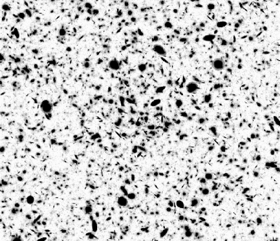
Figure 1: Direct OSIRIS image of the cluster field.

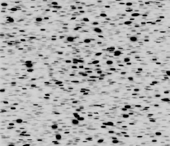
Figure 2: Dispersed image of the same field.

Figure 3 shows instead only an enlargement of the central area of the field. From left to right we show all the galaxies, the field galaxies, and the cluster galaxies. It is clear from the image that it will be possible to discern cluster membership based exclusively in the detection of emission lines. Contamination by other lines will be minimal, with the only possible interlopers being [O 3] 5007Å at much smaller redshift (with a much smaller volume being probed) and Lyman-$\alpha$ at much higher redshift, which will render the galaxies dim enough to be undetected in our images.

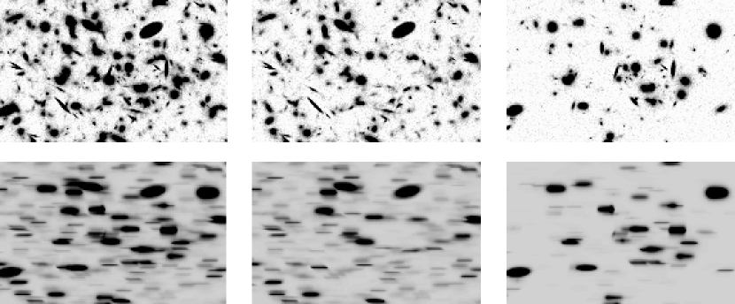
Figure 3: Expanded view of the central area with all galaxies (left), the field (center), and the cluster (right).

Table 1 lists the expected signal-to-noise values with which the continuum and the emission lines would be detected for the objects in our field, as a function of both AB magnitude and equivalent width of the emission line. The magnitude limits that come out of this calculation for detection (S/N=3 per resolution element in three hours) in the dispersed image are AB($V$)=25.5 for the continuum, and AB($V$)=25.1, 25.9, 26.6, 27.3 for an emission line with EW=5, 10, 20, 40 Å respectively.

With these numbers, and using the above-mentioned luminosity functions and EW distributions, we expect to detect up to $\approx$ 100 objects belonging to the cluster in a single OSIRIS image centered in the cluster. This number of objects will represent one of the largest surveys of cluster galaxies ever observed, and constitute by far the largest study to date of a high-redshift cluster.

Table 1: Signal-to-noise calculations

AB($V$)	24.0	25.0	26.0	27.0
(S/N)cont	6.3	2.6	1.0	0.4
(S/N)EW=5Å	4.3	1.8	0.7	0.3
(S/N)EW=10Å	8.4	3.5	1.5	0.6
(S/N)EW=20Å	16.0	6.9	2.9	1.2
(S/N)EW=40Å	29.0	13.0	5.6	2.3

0.3 The next steps

Up to this point we have only presented what we could consider a “single building block” of this project. Several different routes can be followed by appending “building blocks” in different directions. Let us explore some of them:

1- Move towards higher redshift. This is an obvious direction to move to. With the exact same settings presented in the previous section, we would detect $\approx 40$ objects in a $z\approx 0.75$ cluster, and $\approx 20$ in a cluster at $z\approx 1.0$.

2- Move towards larger areas. We can obviously add other fields to the initial one, hereby mosaicing to obtain a larger field and a complete survey of the cluster. An added interest of this project is to study the dynamics of the cluster in the space where its kinematics melts with the Hubble flow. Theoretical studies (Lilje & Lahav 1991) show that it is possible to measure the cosmological parameters using this kind of study.

3- Move to deeper images. This is obviously needed in combination with the first option above, but can also be useful in the original case if deeper study of a particular cluster becomes interesting

4- In any move towards higher redshift, we will be entering the red part of the spectrum, where noise from sky lines becomes dominant. In this case we will need to carefully choose the redshift range to study, and use the tunable filter possibilities to work only in the limited spectral range available between strong sky lines. This is an excellent means of using otherwise “bad”, clear nights.

5- Another improvement will be the use of microslits plus nod-and-shuffle techniques. It will be useful under two different situations: whenever we want to use bright or grey nights (when the sky can be almost completely eliminated by using microslits and sky-free wavelength intervals–otherwise it will dominate the dispersed image), and/or when we have overcrowded fields and have some extra information on which objects we prefer to observe. Glaezebrook and Bland-Hawthorn (2001) show that the gain in sky darkness obtained in this way amounts to a factor of ten reduction in the background.

6- A large improvement will come from the combination of this technique with photometric redshifts. If we can obtain beforehand multi-band images of the field (say $UBVI$, for example) we can perform a photometric redshift analysis in order to eliminate those objects whose colours are clearly incompatible with being at the cluster redshift, and go far deeper by looking only at the “interesting” ones via microslits (as described in 5 above).

References

- [1] Dressler, A., et al. 1999, ApJSS, 122, 51
- [2] Fasano, G., Poggianti, B.M., Couch, W.J., Bettoni, D., Kjærgaard, P. & Moles, M. 2000, ApJ, 542, 673
- [3] Fernández-Soto, A., Lanzetta, K.M. & Yahil, A. 1999, ApJ, 513, 34
- [4] Glazebrook, K. & Bland-Hawthorn J. 2001, PASP, 113, 197
- [5] Lilje, P.B. & Lahav, O. 1991, ApJ, 374, L29
- [6] López-Cruz, O., Yee, H.K.C., Brown, J.P.; Jones, C. & Forman, W. 1997, ApJ, 475, L97
- [7] Smail, I., et al. 1997, ApJSS, 110, 213