Flat Central Density Profiles from Scalar Field Dark Matter Halos

Abstract

Scalar fields endowed with a cosh potential behaves in the linear regime, exactly as the cold dark matter (CDM) model. Thus, the scalar field dark matter (SFDM) hypothesis predicts the same structure formation as the CDM model. The free parameters of the SFDM model are determined by cosmological observations. In a previous work we showed that if we use such parameters, the scalar field collapses forming stable objects with a mass around $10^{12}M_{\odot}$. In the present work we use analytical solutions of the flat and weak field limit of the Einstein- Klein-Gordon equations and show that the SFDM density profile corresponds to a halo with an almost flat central density and that it coincides with the CDM model in a broad outer region. This result could solve the problem of the density cusp DM halo in galaxies without any additional hypothesis, supporting the viability of the SFDM model.

I Introduction

The Lambda Cold Dark Matter ($\Lambda$CDM) model has recently shown an enormous predictive power. It can explain the structure formation of the Universe, its accelerated expansion, the micro Kelvin fluctuation of the Cosmic Microwave Background Radiation, etc. Nevertheless, some issues around this model related to the formation of galaxies have arisen since the time it was originally proposed and remain to date. The CDM paradigm predicts a density profile which corresponds to the Navarro-Frenk-White (NFW) profile, Navarro et al, 1997, given by

$$\rho_{NFW}=\frac{\rho_{0}}{\frac{r}{r_{0}}(\frac{r}{r_{0}}+1)^{2}}.$$ (1)

However, this profile seems to have some differences to the observed profiles of LSB galaxies. In this work we show that a flat central profile naturally arises within the scalar field dark matter hypothesis, implying that the central region of galaxies can distinguish between CDM and SFDM.

We work within the specific context of the so–called ‘strong, self–interacting scalar field dark matter’ (SFDM) hypothesis that has been developed by several authors, Guzmán and Matos 2000, Matos and Ureña-López 2000, 2001; Ureña-López, Matos and Becerril 2002; Matos and Guzmán 2001; Alcubierre et al. 2002, 2003; Ureña-López 2002; Böhmer and Harko 2007; (see also Peebles 2000). A first proposal of the SFDM hypothesis appeared in a couple of papers by Ji and Sin 1994. They took a massive scalar field and were able to fit observations comming from some galaxies, taken into account also the contribution of baryons. A key point in this work was the use of the so-called excited configurations in which the radial profile of the scalar fields has nodes. From that, they determined that the mass of the scalar field should be of order of $\sim 10^{-24}$ eV.

A next proposal appeared in a paper by Schunck 1998. He shows that a massless complex scalar field can be used as a dark matter model in galaxies to fit the rotation curves. In this model the internal frequency of the field plays the role of an adjustable parameter, and the radial profile of the scalar field also has nodes.

However, as pointed out in Guzmán and Ureña-López 2005 (see also Guzmán and Ureña-López 2004), this last proposal cannot be realistic because a massless scalar field (whether real or complex as in Schunck 1998) cannot form a gravitationally bound configuration (see Seidel and Suen 1994).

The key idea of the SFDM scenario is that the dark matter responsible for structure formation in the Universe is a real scalar field, $\Phi$, minimally coupled to Einstein gravity with self-interaction parametrized by a potential energy of the form (see also Sahni and Wang 2000)

$$V(\Phi)=V_{0}\left[\cosh(\lambda\sqrt{\kappa_{0}}\Phi)-1\right],$$ (2)

where $V_{0}$ and $\lambda$ are the only two free parameters of the model, $\kappa_{0}=8\pi G$ and we employ natural units $\hbar=c=1$. The effective mass of the scalar field is given by $m_{\Phi}^{2}=\kappa_{0}V_{0}\lambda^{2}$.

The advantage of the SFDM model is that it is insensitive to initial conditions and the scalar field behaves as CDM once it begins to oscillate around the minimum of its potential. In this case, it can be shown (see Matos and Ureña-López 2000, 2001) that the SFDM model is able to reproduce all the successes of the standard $\Lambda$CDM model above galactic scales.

Furthermore, it predicts a sharp cut-off in the mass power spectrum due to its quadratic nature, thus explaining the observed dearth of dwarf galaxies, in contrast with the possible excess predicted by high resolution N-body simulations with standard CDM, see Matos and Ureña-López 2001.

The best–fit model to the cosmological data can be deduced from the current densities of dark matter and radiation in the Universe and from the cut–off in the mass power spectrum that constrains the number of dwarf galaxies in clusters. The favored values for the two free parameters of the scalar field potential are found to be, Matos and Ureña-López 2001:

$$\lambda \simeq 20,$$

$$V_{0} \simeq (3\times 10^{-27}\,m_{Pl})^{4}\,,$$ (3)

where $m_{Pl}\equiv G^{-1/2}\approx 10^{-5}$g is the Planck mass.

This implies that the effective mass of the scalar field should be $m_{\Phi}\simeq 9.1\times 10^{-52}\,m_{Pl}=1.1\times 10^{-23}$ eV.

Let us explain why we suspect that the scalar field could be the dark matter at galactic scales as well. There are three main reasons.

The first reason is that numerical simulations suggest that the critical mass for the case considered here, using the scalar potential (2), and the parameters given by Eq. (3), is approximately, Alcubierre et. al. 2002

$$M_{crit}\simeq 0.1\frac{m_{Pl}^{2}}{\sqrt{\kappa_{0}V_{0}}}=2.5\times 10^{13}M_{\odot}\,.$$ (4)

This was a surprising result. The critical mass of the model shown in Matos and Ureña-López 2000, 2001, is of the same order of magnitude of the dark matter content of a standard galactic halo. Observe that the parameters of the model, Eq. (3), were fixed using cosmological observations. The surprising result consisted in the fact that using the same scalar field for explaining the dark matter at cosmological scales, it will always collapse with a preferred mass which corresponds to the halo of a real galaxy. Thus, this result is a prediction of the cosmological SFDM model for galaxy formation.

The second reason is that during the linear regime of cosmological fluctuations, the scalar field and a dust fluid, like CDM, behave in the same way. The density contrast in CDM and in the SFDM models evolve in exactly the same form and then both models predict the same large scale structure formation in the Universe (see Matos and Ureña-López 2001). The differences between the CDM and SFDM models begin to appear in the non linear regime of structure formation, so that there will be differences in their predictions on galaxy formation.

The third reason is the topic of this work. A scalar field object (e.g. an oscillaton) contains a flat central density profile, as seems to be the case in galaxies.

In the case of the SFDM, the strong self-interaction of the scalar field results in the formation of solitonic objects called ‘oscillatons’, which have a mass of the order of a galaxy (see for example Ureña-López 2002, Ureña-López et al 2002 and Alcubierre et al 2003. Also Seidel and Suen 1991, 1994, Hawley and Choptuik 2000, and Honda and Choptuik 2001). In this work we will show that these models contain an almost flat central density profile, ${\it i.e.}$, they do not exhibit the cusp density profiles characteristic of the standard CDM hypothesis.

Before starting with the description, we want to emphazise the fact that the scalar field has no interaction with the rest of the matter, thus, it does not follow the standard lines of reasoning for the particle-like candidates for dark matter. The scalar field was not thermalized, that is, the scalar field forms a Bose condensate, and thus behaves strictly as cold dark matter from the beginning.

The rest of the paper is organized as follows. In the next section we use the fact that Galaxies have a weak gravitational field and thus their space-time is almost flat. The main goal of this section is to study the physics provoking the flatness behavior of the density profiles at the center of the oscillatons. Some results of this section intersect with those presented by Jin and Sin 1994, where they studied the behavior of the weak field limit of a complex scalar field. We remark that we do our analysis for a real scalar field and some differences do arise due to a different current conservation. In section III we present our contribution making an analysis of the Einstein-Klein-Gordon (EKG) equations in the relativistic weak field limit and solve them for the perturbed metric coefficients. Then, we compare these solutions with the ones obtained by solving numerically the complete EKG system and using the whole potential (2), we show that the relativistic weak field limit is indeed a very good approximation. In section IV we compute the energy density of the scalar field obtained in section III, and compare it with actual observations of LSB galaxies from which the density is inferred from the rotational curves, showing a good matching in the external regions and a match at least similar in some of the internal regions, in any case, better than a fit with a cusp-like behavior of the density. Finally in section V we give our conclusions.

II Physics of the Scalar Field. Flat space-time case

In this section we derive the physics of the scalar field in an analogous way as it was done for the complex scalar field by Jin and Sin 1994 (see also Lee and Koh 1996). In a normal dust collapse, as for example in CDM, there is in principle nothing to avoid that the dust matter collapses all the time. There is only a radial gravitational force that provokes the collapse, and to stop it, one needs to invoke some virialization phenomenon. In the scalar field paradigm the collapse is different. The energy momentum tensor of the scalar field is

$$T_{\mu\nu}=\Phi_{,\mu}\Phi_{,\nu}-\frac{g_{\mu\nu}}{2}\,\left[\Phi^{,\alpha}\Phi_{,\alpha}+2V(\Phi)\right]\,.$$ (5)

We will consider spherical symmetry, and work with the line element

$$ds^{2}=-e^{2\nu}dt^{2}+e^{2\mu}dr^{2}+r^{2}d\Omega^{2}\,,$$ (6)

with $\mu=\mu(r,t)$ and $\nu=\nu(r,t)$, being this last function the Newtonian potential. The energy momentum tensor of the scalar field has then the components

$$-{T^{0}}_{0}=\rho_{\Phi}=\frac{1}{2}\left[e^{-2\nu}{\dot{\Phi}}^{2}+e^{-2\mu}\Phi^{\prime 2}+2V(\Phi)\right]$$ (7)

$$T_{01}={\cal P}_{\Phi}=\dot{\Phi}\Phi^{\prime}$$ (8)

$${T^{1}}_{1}=p_{r}=\frac{1}{2}\left[e^{-2\nu}{\dot{\Phi}}^{2}+e^{-2\mu}\Phi^{\prime 2}-2V(\Phi)\right]$$ (9)

$${T^{2}}_{2}=p_{\bot}=\frac{1}{2}\left[e^{-2\nu}{\dot{\Phi}}^{2}-e^{-2\mu}\Phi^{\prime 2}-2V(\Phi)\right]$$

and also ${T^{3}}_{3}={T^{2}}_{2}$. These different components are identified as the energy density $\rho_{\Phi}$, the momentum density ${\cal P}_{\Phi}$, the radial pressure $p_{r}$ and the angular pressure $p_{\bot}$. The integrated mass is defined by

$$M(x)=4\pi\int_{0}^{x}\rho_{\Phi}(X)\,X^{2}dX\,.$$ (11)

The radial and angular pressures are two natural components of the scalar field which stop the collapse, avoiding the cusp density profiles in the centers of the collapsed objects. This is the main difference between the normal dust collapse and the SFDM one. The pressures play an important roll in the SFDM equilibrium. In order to see this, and considering that galaxies are almost flat, we conclude that the Newtonian approximation should be sufficient to describe the processes. In this section we will take the flat space-time approximation.

Thus, we study a massive oscillaton without self-interaction ($i.e.$ with potential $V=\frac{1}{2}m_{\Phi}^{2}\Phi^{2}$), in the Minkowski background ($\mu\sim\nu\sim 0$). Even though it is not a solution to the Einstein equations as we are neglecting the gravitational force provoked by the scalar field, the solution is analytic and it helps us to understand some features that appear in the non-flat oscillatons.

In a spherically symmetric space-time, the Klein-Gordon equation $\eta^{\alpha\beta}\partial_{\alpha}\partial_{\beta}\,\Phi-dV/d\Phi=0$, (where $\eta^{\alpha\beta}\partial_{\alpha}\partial_{\beta}$ stands for the D’Alambertian), reads

$$\Phi^{\prime\prime}+\frac{2}{r}\Phi^{\prime}-m_{\Phi}^{2}\Phi=\ddot{\Phi},$$ (12)

where over-dot denotes $\partial/\partial t$ and prime denotes $\partial/\partial r$. The exact general solution for the scalar field $\Phi$ is

$$\Phi(t,r)=\frac{e^{\pm ikr}}{r}e^{\pm i\omega t},$$ (13)

and we obtain the dispersion relation $k^{2}=\omega^{2}-m_{\Phi}^{2}$. For $\omega>m_{\Phi}$ the solution is non-singular and vanishes at infinity. We will restrict ourselves to this case. It is more convenient to use trigonometric functions and to write the particular solution in the form

$$\Phi(t,x)=\Phi_{0}\frac{\sin(x)}{x}\cos(\omega t),$$ (14)

where $x=kr$. It oscillates in harmonic manner in time. The scalar field can be considered to be confined to a finite region, see Ureña-López 2002, and Ureña-López et al 2002.

Figure 1: The energy density profile for the Scalar Field Dark Matter model (see also Schunck 1997). The parameters used in this plot are $m_{\Phi}=20,\omega=20.001,\Phi_{0}^{2}=5\ 10^{-2}$. The density is given in arbitrary units and $r$ is given in kpc.

The analytic expression for the scalar field energy density derived from Eq. (14) is

$$\rho_{\Phi}= \frac{{\Phi_{0}}^{2}\,k^{2}}{2\,x^{2}}\left[\left(\left(\frac{\sin(x)}{x}-\cos(x)\right)^{2}\right.\right.$$

$$\left.\left.-k^{2}\,\sin^{2}(x)\right)\,\cos^{2}(\omega\,t)+\omega^{2}\,\sin^{2}(x)\right],$$

which oscillates with a frequency $2\omega t$. Observe that close to the central regions of the object, the density of the oscillaton behaves like

$$\rho_{\Phi}\sim\frac{1}{2}{\Phi_{0}}^{2}k^{2}\left[\omega^{2}-k^{2}\cos^{2}\left(\omega\,t\right)\right]+O(x^{2}),$$ (16)

which implies that when $x\rightarrow 0$ the central density oscillates around a fixed value.

On the other hand, the asymptotic behavior when $x\rightarrow\infty$, is such that $\rho_{\Phi}\sim 1/x^{2}$, $i.e.$ far away from the center, in this approximation, the flat oscillaton density profile behaves like the isothermal one. The mass function oscillates around $M\sim x$, as usual for the galactic halos.

In order to understand what is happening within the object, observe that the KG equation can be rewritten in a more convenient form in terms of the energy density, as

$$\frac{\partial\rho_{\Phi}}{\partial t}-\frac{1}{r^{2}}\frac{\partial}{\partial r}\left(r^{2}{\cal P}_{\Phi}\right)=0.$$ (17)

This last equation has a clear interpretation: Since its form looks like the conservation equation, $\dot{\rho}+\nabla\cdot\vec{J}=0$, equation (17) represents the conservation of the scalar field energy. It also tells us that there is a scalar field current given by

$$\vec{J}_{\Phi} = -{\cal P}_{\Phi}\vec{r}$$

$$= \Phi_{0}^{2}\frac{k\omega}{2}\left[x\cos(x)-\sin(x)\right]\frac{\sin(x)\sin(2\omega t)}{x^{3}}\vec{r}.$$

Observe that the quantity involved in this current is the scalar field momentum density (8). Although the flux of scalar radiation at large distances does not vanish, there is not a net flux of energy, as it can be seen by averaging the scalar current on a period of a scalar oscillation. We also see that the only transformation process is that of the scalar field energy density into the momentum density, and viceversa. For the realistic values (3) this transfer is very small.

In Fig. 1 we show the behavior of the SFDM density profile for a typical galaxy and in Fig. 2 we show the comparison between the NFW, the isothermal and the SFDM density profiles for the same galaxy. Observe that the SFDM and NFW profiles remain very similar up to 10 kpc, then the SFDM profile starts to follow the isothermal one.

Figure 2: Comparison between the energy density profile for the Scalar Field Dark Matter model with the NFW and the Isothermal models. The parameters for the isothermal model are $\rho_{Iso}=0.3/(r^{2}+8^{2})$ and for the NFW profile are $\rho_{NFW}=10/(r(r+8)^{2})$. The parameter used for the SFDM model are the same as in the previous figure.

In the next section we will see that if the gravitational force is taken into account, the oscillaton is more confined (see also Ureña-López 2002, Ureña-López et al 2002, and Alcubierre et al 2003). The parameters used in the figures, correspond to a middle size galaxy.

III Weak Field Limit Equations

In this section we derive a novel method for integrating the perturbed EKG equations and show that the solutions are in very good agreement with the numerical ones. This allow us to use these solutions to fit the rotation curves of several observed LSB galaxies.

Within general relativity, the evolution of the scalar and gravitational fields are governed by the coupled EKG equations, the last one appearing from the conservation of the energy-momentum tensor

$$R_{\alpha\beta} = \kappa_{0}S_{\alpha\beta},$$ (18)

$$T^{\alpha\beta};_{\beta} = \Phi^{,\alpha}(\nabla^{2}-m^{2})\Phi=0,$$ (19)

here $R_{\alpha\beta}$ is the Ricci tensor, $S_{\alpha\beta}=T_{\alpha\beta}-(1/2)g_{\alpha\beta}T^{\lambda}_{\phantom{\lambda}\lambda}$, and $\nabla^{2}=(1/\sqrt{-g})\partial_{\mu}[\sqrt{-g}g^{\mu\nu}\partial_{\nu}]$ is the covariant D’Alambertian operator.

For simplicity, we continue to consider the non-static spherically symmetric case, given by Eq. (6). As usual in the weak field limit, we suppose the metric to be close to the Minkowski metric $\eta_{\alpha\beta}$

$$g_{\alpha\beta}=\eta_{\alpha\beta}+h_{\alpha\beta},$$ (20)

where $|h_{\alpha\beta}|\ll 1$, then we will consider an expansion of the functions in the metric of the form

$$e^{2\nu(t,r)}=1+\epsilon^{2}2V(t,r)+O(\epsilon^{4}),$$

$$e^{2\mu(t,r)}=1+\epsilon^{2}2U(t,r)+O(\epsilon^{4}),$$ (21)

where $\epsilon$ is an expansion parameter. We also consider that the spatial and time derivatives of the geometric quantities are regarded like

$$\frac{\partial}{\partial t}\sim\frac{\partial}{\partial r}.$$ (22)

then to first order in $\epsilon^{2}$ the Ricci tensor components are respectively

$$R_{tt} = [V,_{rr}-U,_{tt}+\frac{2}{r}V,_{r}],$$

$$R_{rr} = [U,_{tt}-V,_{rr}+\frac{2}{r}U,_{r}],$$

$$R_{tr} = [\frac{2}{r}U,_{t}].$$ (23)

On the other hand, the source is computed in the flat space in this case as well, thus the scalar field satisfies to $\epsilon^{2}$ order the Eq. (12) as in the previous section.

It is important to emphasize that the relation (22) is the lowest one in the geometric fields, but it does not consider small velocities for the sources. This is different from the Newtonian limit where the derivative relation for the scalar field is $\partial_{r}\sim\epsilon\partial_{t}$ and $\partial_{t}\sim\epsilon\partial_{r}$ for the geometric fields (see Seidel & Suen 1990, and Guzmán & Ureña-López 2004).

Consistent with the $T_{\alpha\beta}$ computed in the flat space-time, the right hand side elements in Einstein’s equations, are written as

$$S_{tt} = \Phi,_{t}\Phi,_{t}-\frac{1}{2}m^{2}|\Phi|^{2},$$

$$S_{rr} = \Phi,_{r}\Phi,_{r}+\frac{1}{2}m^{2}|\Phi|^{2},$$

$$S_{tr} = \Phi,_{r}\Phi,_{t}.$$ (24)

In this case it is convenient to introduce the dimensionless quantities

$$x=mr,\quad\tau=mt,\quad\Omega=\frac{\omega}{m},$$ (25)

where we note that the bosonic mass $m$ is the natural scale for time and distance. In terms of these new variables the general solution to Eq. (13) takes the form

$$\Phi(\tau,x)=\frac{1}{x}\exp(\pm ix\sqrt{\Omega^{2}-1})\exp(\pm i\Omega\tau).$$ (26)

The physical properties of the solution depend on the ratio $\Omega\equiv\omega/m$. For $\Omega<1$ the solution decays exponentially but it is singular at $r=0$. On the other hand, $\Omega>1$ allows for non-singular solutions which vanish at infinity. We will restrict ourselves to this case. We will write the particular solution in the form

$$\sqrt{\kappa_{0}}\Phi(\tau,x)=\phi(x)\cos(\Omega\tau),$$ (27)

where the spatial function is given by

$$\phi(x)=\phi_{0}\frac{\sin(x\sqrt{\Omega^{2}-1})}{x}.$$ (28)

Because of the functional form of the scalar field (27) we introduce the following ansatz for the metric perturbations (III)

$$V(\tau,x) = V_{0}(x)+V_{2}(x)\cos(2\Omega\tau),$$

$$U(\tau,x) = U_{0}(x)+U_{2}(x)\cos(2\Omega\tau).$$ (29)

We adopt the following method to solve the EKG equations. In the first approximation we substitute the solution of a lower approximation (the flat case) into the next approximation (with $\epsilon^{2}$) and solve the resulting differential equations. As we will see, this standard approximation works well in our case. In terms of these expressions the Einstein’s equations $R_{\alpha\beta}=\kappa_{0}S_{\alpha\beta}$ finally read

$$\epsilon^{2}\left[\frac{4}{x}U_{2}\right] = \frac{1}{2}\phi\phi,_{x},$$ (30)

$$\epsilon^{2}\left[V_{0},_{xx}+\frac{2}{x}V_{0},_{x}\right] = \frac{1}{2}\left(\Omega^{2}-\frac{1}{2}\right)\phi^{2},$$

$$\epsilon^{2}\left[V_{2},_{xx}+\frac{2}{x}V_{2},_{x}+4\Omega^{2}U_{2}\right] = -\frac{1}{2}\left(\Omega^{2}+\frac{1}{2}\right)\phi^{2},$$

$$\epsilon^{2}\left[-V_{0},_{xx}+\frac{2}{x}U_{0},_{x}\right] = \frac{1}{2}\left(\phi,_{x}^{2}+\frac{1}{2}\phi^{2}\right),$$

$$\epsilon^{2}\left[-V_{2},_{xx}+\frac{2}{x}U_{2},_{x}-4\Omega^{2}U_{2}\right] = \frac{1}{2}\left(\phi,_{x}^{2}+\frac{1}{2}\phi^{2}\right).$$

III.1 Scaling properties

From system (30) we know that the scalar field’s maximum amplitude $\phi(0)=\phi_{0}\sqrt{\Omega^{2}-1}$ could be taken as the expansion parameter $\epsilon$ and in this case $\Omega$ must be of order $1$. Then it is always possible to solve the system (30) ignoring $\epsilon$ and replacing $\phi$ by its normalized function

$$\hat{\phi}(x)=\frac{\sin(x\sqrt{\Omega^{2}-1})}{x\sqrt{\Omega^{2}-1}}.$$ (31)

Solutions $\hat{\phi}$, $U_{0}$, $U_{2}$, $V_{0}$, $V_{2}$ of this normalized system depend only of the arbitrary characteristic frequency $\Omega$ which modulate the wave length of $\hat{\phi}$. On the other hand, for each value of $\Omega$ there is a complete family of solutions of the scalar field $\phi$ and the metric perturbations $h_{\alpha\beta}$ which are related to each other by a scaling transformation characterized by $\phi_{0}$

$$\sqrt{\kappa_{0}}\Phi = \phi_{0}\sqrt{\Omega^{2}-1}\hat{\phi}\cos(\Omega\tau),$$ (32)

$$h_{rr} = \phi_{0}^{2}(\Omega^{2}-1)[2U_{0}+2U_{2}\cos(2\Omega\tau)],$$

$$h_{tt} = -\phi_{0}^{2}(\Omega^{2}-1)[2V_{0}+2V_{2}\cos(2\Omega\tau)],$$

In this context the weak field limit condition $h_{\alpha\beta}\ll 1$ translates into

$$\phi_{0}^{2}(\Omega^{2}-1)|2V|\ll 1,\quad\&\quad\phi_{0}^{2}(\Omega^{2}-1)|2U|\ll 1.$$ (33)

Here we will introduce a specific notation for the spatial functions of the metric perturbations:

$$h_{rr}^{(0)} = \phi_{0}^{2}(\Omega^{2}-1)2U_{0},$$ (34)

$$h_{rr}^{(2)} = \phi_{0}^{2}(\Omega^{2}-1)2U_{2},$$

$$h_{tt}^{(0)} = \phi_{0}^{2}(\Omega^{2}-1)2V_{0},$$

$$h_{tt}^{(2)} = \phi_{0}^{2}(\Omega^{2}-1)2V_{2}.$$

III.2 Metric perturbations solutions

The system of equations Eqs. (30) can be solved and the spatial functions of the metric perturbations have analytic solutions given by

$$U_{2}=\frac{1}{8(\Omega^{2}-1)}\Big{[}-\frac{\sin^{2}(x\sqrt{\Omega^{2}-1})}{x^{2}}+{}$$

$${}+\frac{\sqrt{\Omega^{2}-1}}{2}\frac{\sin(2x\sqrt{\Omega^{2}-1})}{x}\Big{]},$$

$$V_{0}=\frac{(2\Omega^{2}-1)}{8(\Omega^{2}-1)}\Big{[}\frac{\sin(2x\sqrt{\Omega^{2}-1})}{2x\sqrt{\Omega^{2}-1}}-{}$$

$${}-Ci(2x\sqrt{\Omega^{2}-1})+{}$$

$${}+\ln(2x\sqrt{\Omega^{2}-1})\Big{]}-\frac{C_{V01}}{x}+C_{V02},$$

$$V_{2}=\frac{1}{8(\Omega^{2}-1)}\Big{[}\frac{\sqrt{\Omega^{2}-1}}{2}\frac{\sin(2x\sqrt{\Omega^{2}-1})}{x}+{}$$

$${}+Ci(2x\sqrt{\Omega^{2}-1})-{}$$

$${}-\ln(2x\sqrt{\Omega^{2}-1})\Big{]}+C_{V22},$$

$$U_{0}=\frac{1}{8(\Omega^{2}-1)}\Big{[}-\frac{1}{2x^{2}}+\frac{1}{2}\frac{\cos(2x\sqrt{\Omega^{2}-1})}{x^{2}}-{}$$ (35)

$${}-\frac{1}{2}\frac{\sin(2x\sqrt{\Omega^{2}-1})}{x\sqrt{\Omega^{2}-1}}\Big{]}+\frac{C_{V01}}{x}+C_{U01},$$

where $Ci$ is the cosine integral function and $C_{V01}$, $C_{V02}$, $C_{V22}$, and $C_{U01}$ are integration constants.

III.3 Weak Field Validity Range

From equation (13) it is evident that, in the limit in which we are working with, the KG equation is decoupled from Einstein equations. Imposing regularity at the origin and asymptotic flatness to the KG solution we have chosen (27) with (28) as our scalar field particular solution where $\phi_{0}$ and $\Omega>1$ are still free parameters.

On the other hand, regularity at $x=0$ requires $h_{rr}(x=0,\tau)=0$ which implies

$$C_{V01}=0,\quad C_{U01}=\frac{\Omega^{2}}{8(\Omega^{2}-1)},$$ (36)

then for the perturbations $C_{V02}$ and $C_{V22}$ are still free integration constants. Now we will describe the asymptotic behavior of these perturbations. Due to $U_{2}$ being at least one order of magnitude smaller than $U_{0}$ and its value oscillating around zero, it is $U_{0}$ which determines the behavior of $h_{rr}$. The $U_{0}$ value starts to oscillate, very near to the origin, around $C_{U01}$ keeping this behavior asymptotically. Then the asymptotic value of $h_{rr}$ is the finite $C_{U01}$ value. Contrary to this $h_{tt}$, due to the logarithm terms in $V_{0}$ and $V_{2}$, $h_{tt}$, is singular at infinity. Thus, the weak field condition (33) is fulfilled only in a finite spatial region around the origin, $i.e.$, due the the approximation the solution is contained in a box, for which the walls are sufficiently far away from the center of the solution. We will say that this is the region where our weak field approximation is valid.

Unique solutions for the EKG system will be obtained fixing the $\phi_{0}$ and $\Omega$ parameters and the constants $C_{V02}$ and $C_{V01}$ within the validity range of the approximation. As it is known the potentials measurement does not have physical sense by themselves, then unique solutions will be determined through metric dependent observable quantities. Using the expressions given by Eqs. (34), we can obtain the perturbed metric functions in terms of these solutions. In Fig. 3 we present a plot of these metric perturbation functions, as well as of the scalar field, for two values of $\Omega$.

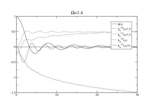
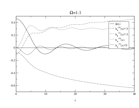
Figure 3: Profiles of $\phi(x)$, $h_{rr}^{(2)}(x)$, $h_{rr}^{(0)}(x)$,$h_{tt}^{(2)}(x)$ and $h_{tt}^{(0)}(x)$ with $\phi_{0}=1$; see text for details.

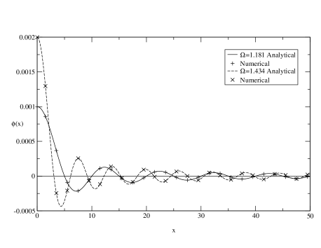
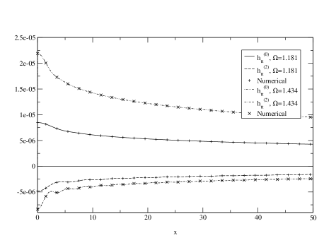
Figure 4: (Left) Spatial function $\phi$ of the scalar field $\Phi$. Solid and dash lines are analytical solutions with $\phi_{0}=0.001/\sqrt{(\Omega^{2}-1)}=0.001591$, and $\phi_{0}=0.002/\sqrt{(\Omega^{2}-1)}=0.001946$, respectively. The crosses are the corresponding numerical solutions with $\phi_{1}(0)=0.001$, $\Omega=1.181008$ and $\phi_{1}(0)=0.002$, $\Omega=1.433822$; see text for details. (Right) Spatial functions $h_{tt}^{(0)}$ and $h_{tt}^{(2)}$ of the metric perturbations.

It is important to mention that the width of the validity region, where (33) is fulfilled, depends on $\Omega$ and $\phi_{0}$. This is because it is the factor $\phi_{0}^{2}$ which modulate the perturbations, (see (32)). What it is not evident until the solutions (III.2) are observed is that the $\Omega$ value, independently from $\phi_{0}$, could make the validity range width bigger. This is because in the logarithm argument there is the expression $\sqrt{\Omega^{2}-1}$, then as $\Omega$ is closer to one the logarithm terms rise more slowly.

The order of magnitude for the other parameter $\phi_{0}$ in the metric perturbations, can be naturally determined from the asymptotic value taken by $h_{rr}$, which is reached very close to the origin

$$\lim_{x\to\infty}|h_{rr}|=\frac{\phi^{2}_{0}}{4}\Omega^{2}.$$ (37)

As $\Omega$ is nearly $1$ the $h_{rr}$ magnitude is given by $\phi_{0}$. It is well known that for week field systems like our Solar System the metric perturbations go like $h_{\alpha\beta}\sim 10^{-6}$. This value restricts our $\phi_{0}$ to be $\phi_{0}\lesssim 10^{-3}$.

III.4 Analytical Solutions vs Numerical Solutions

Analytic solutions $\phi_{0}$, $h_{rr}^{(2)}(x)$, $h_{rr}^{(0)}(x)$, $h_{tt}^{(2)}(x)$ and $h_{tt}^{(0)}(x)$ are shown in Fig. 3. The value of $\phi_{0}$ is $1$ in both plots. As already was noticed, the value of $\Omega$ characterizes each family of solutions. Mainly $\Omega$ determines the wave length of $\phi$ and the increase rate of $h_{tt}^{(0)}$ and $h_{tt}^{(2)}$; as $\Omega$ is closer to $1$ this rate is smaller. These characteristics are shown in Fig. 3.

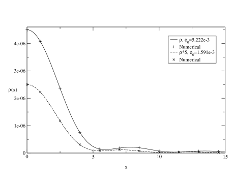
Figure 5: (Left) Energy-Momentum density profiles for two scalar field configurations one with $\phi_{0}=1.1591\,\,10^{-3}$ and $\Omega=1.181008$ and the other with $\phi_{0}=5.2225\,\,10^{-3}$ and $\Omega=1.153246$. (Right) Difference between density profiles from the exact EKG equations ($\rho_{N}$) and the density computed in the flat space-time ($\rho$); see text for details.

The exact EKG equations in spherical symmetry with a quadratic potential, were solved numerically in Ureña-López 2002, and Ureña-López et al 2002) and found the so called oscillatons. In those works boundary conditions are determined by requiring non-singular and asymptotically flat solutions, for which the EKG become an eigenvalue problem. The free eigenvalue is the scalar field’s central value $\phi_{1}(x=0)$ which labels the particular equilibrium configuration, and the fundamental frequency $\Omega$ is an output value. In those works it is also noted that weak gravity fields are produced by oscillatons with $\phi_{1}(x=0)\ll 1$. In Fig. 4 we compare some of these numerical solutions (NS) with the analytical solutions (AS) within a central region. The constant values of the AS are fixed to fit better the NS inside the weak field validity range. From these plots we can conclude that our solutions are a very good approximation for the exact EKG equations in the weak field limit. The principal advantage of this approximation is the analytical description of the solutions.

IV Scalar Field as Dark Matter: Halo Density Profile

In this section we explore whether or not the scalar field could account as the galactic DM halos. Specifically we compare the SFDM model density profile and the profiles inferred throughout the rotation curves profiles of galaxies which are mostly formed by DM.

As long as we are concerned with perturbations of the flat space-time due to the scalar field, we do not consider the baryonic matter gravitational effects, we expect that our approximation will be better suited for galaxies with very small baryonic component.

We will compare the energy-momentum density for the scalar field given by Eq. (7), in the relativistic weak limit approximation, where for the metric functions, Eq.(III), we use the solutions to the perturbations given by Eqs. (29,III.2).

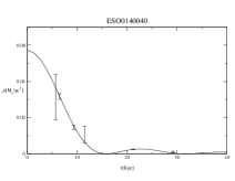
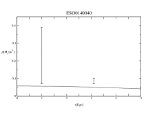
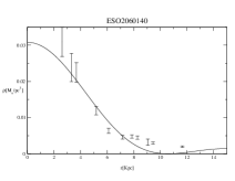
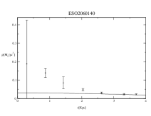
Figure 6: Density profile fits for the galaxies ESO0140040, ESO2060140, the right panel is a zoom of its central region, it is plotted in order to visualize complete error bars. The horizontal line is in $kpc$, vertical line in $M_{\odot}/pc^{3}$. See text and Table  1 for fit details.

This is consistent with the fact that gravity does not modify the scalar field behavior. This approximation in the weak gravitational field limit is very good as we can see in Fig.  5. In those plots we show the energy-momentum density profiles for two scalar field configurations with different maximum amplitudes at the origin $\phi(0)=\phi_{0}\sqrt{\Omega^{2}-1}$. It is important to notice that as $\phi(0)$ decreases the gravitational field gets weaker, and the difference between the density from the complete EKG equations and from our approximation is smaller.

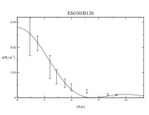
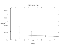
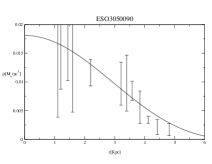
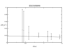
Figure 7: The same as Fig. 6, but for the galaxies ESO3020120, ESO3050090.

The density profile fits allow us to obtain an estimation of the parameters at the galactic level: the fundamental frequency $\Omega$ and the scalar field constant $\phi_{0}$. The third parameter involved in the density profiles is the scalar field mass, we will fix it to be $m=10^{-23}$ eV. This value was fitted for the SFDM model from cosmological observations in Matos & Ureña-López 2001.

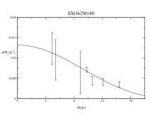
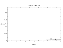
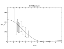
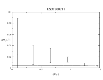
Figure 8: The same as Fig. 6, but for the galaxies ESO4250180, ESO1200211.

IV.1 Density Profile fits

The first qualitative feature of the energy-density profile that we want to emphasize is that in the central region it is non cuspy (see Fig. 5). It is important to take into account that instead of density profiles, rotation curves are the direct observable for galaxies. Nevertheless, for galaxies dominated by DM, their rotation curves could model the DM density profile more trustfully. We choose a subset of galaxies from the set presented in McGaugh 2001, the common characteristic for the selected galaxies is that the luminous matter velocity contribution to the rotation curves is almost null.

With the scalar field mass $m$ fixed, the profiles fits were made for the $\Omega$ and $\phi_{0}$ values with good $\chi^{2}$ statistic, see Table  1. In most of the cases the non central observational data were the good fitted points, those data points also have smaller error bars. The density profile fits are in Figures 6,7,8,9, where we show several galaxies with the density computed from the observed rotational profile versus the density obtained with our SFDM description. In some of them we were able to compare regions within less than $0.5$ Kpc.

In Table 1 the fundamental frequency $\Omega$ is listed for each galaxy. We found that the temporal dependence for the energy-momentum density profile is harmonic with a temporal period $T=\pi/\Omega$. The column $\Delta\rho(0)$ corresponds to the maximum change in the central density for a period of time $T$. Finally for all the galaxies the $\phi_{0}$ value is well inside of the weak gravitation field limit $\phi_{0}\lesssim 10^{-3}$.

Table 1: Galactic Parameter Values

Galaxy	$\Omega$	$\phi_{0}$	$\chi^{2}$	$\rho(r=0)$	$\Delta\rho(0)$	$T$
				$[M_{\odot}/pcs^{3}]$	$[M_{\odot}/pcs^{3}]$	$[yrs]$
ESO0140040	$1+8\,\,\,10^{-9}$	$1.87\,\,10^{-3}$	$12.366$	$0.569\,\,10^{-1}$	$0.755\,\,10^{-8}$	$1.603382750\,\,10^{7}$
ESO0840411	$1+6\,\,10^{-9}$	$5.95\,\,10^{-4}$	$1.338$	$0.433\,\,10^{-2}$	$0.147\,\,10^{-9}$	$1.603953416\,\,10^{7}$
ESO1200211	$1+53\,\,10^{-9}$	$2.04\,\,10^{-4}$	$10.062$	$0.448\,\,10^{-2}$	$0.530\,\,10^{-9}$	$1.603382679\,\,10^{7}$
ESO1870510	$1+12\,\,10^{-9}$	$3.28\,\,10^{-4}$	$3.190$	$0.265\,\,10^{-1}$	$0.699\,\,10^{-8}$	$1.603382570\,\,10^{7}$
ESO2060140	$1+18\,\,10^{-9}$	$9.18\,\,10^{-4}$	$65.421$	$0.308\,\,10^{-1}$	$0.206\,\,10^{-8}$	$1.603382735\,\,10^{7}$
ESO3020120	$1+29\,\,10^{-9}$	$6.88\,\,10^{-4}$	$16.099$	$0.279\,\,10^{-1}$	$0.170\,\,10^{-8}$	$1.603382718\,\,10^{7}$
ESO3050090	$1+40\,\,10^{-9}$	$4.72\,\,10^{-4}$	$1.224$	$0.181\,\,10^{-1}$	$0.243\,\,10^{-8}$	$1.603382699\,\,10^{7}$
ESO4250180	$1+4\,\,10^{-9}$	$1.27\,\,10^{-3}$	$5.221$	$0.132\,\,10^{-1}$	$0.105\,\,10^{-8}$	$1.603382757\,\,10^{7}$
ESO4880049	$1+3\,\,10^{-9}$	$7.86\,\,10^{-4}$	$11.410$	$0.377\,\,10^{-1}$	$0.212\,\,10^{-8}$	$1.603382715\,\,10^{7}$

V Conclusions and Future Prospects

We have found analytic solutions for the EKG equations, for the case when the scalar field is consider as a test field in a Minkowski background, and in the relativistic weak gravitational field limit at first order in the metric perturbations. With these solutions we have shown that non-trivial local behavior of the scalar field holds the collapse of an object formed from scalar field matter. The scalar field contains non trivial, natural effective pressures which stop the collapse and prevent the centers of these objects from having cusp-lke density profiles. Even within this simple approximation it has been possible to fit, with relative success, the density profiles for some galaxies showing non cuspy profiles.

Together, all the features of the SFDM model allow one to consider this model as a robust alternative candidate to be the dark matter of the Universe, as was suggested by Guzmán and Matos 2000, Matos and Guzmán 2000, 2001, and Matos et al 2000. Furthermore, it has been shown previously that dark halos of galaxies could be scalar solitonic objects, even in the presence of baryonic matter, Hu et al 2000; Lee and Koh 1996; Arbey et al 2001, 2002; Sin 1994; and Ji and Sin 1994. Actually, the boson mass estimated in all these different approaches roughly coincides with the value $m_{\Phi}\sim 10^{-23}eV$, even if the later was estimated from a cosmological point of view, Matos and Ureña-López 2001. We can appreciate the non-trivial characteristics of the proposed potential (2): Its strong self-interaction provides a reliable cosmological scenario, while at the same time it has the desired properties of a quadratic potential. Finally, the results presented here fill the gap between the successes at cosmological and galactic levels.

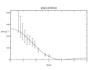
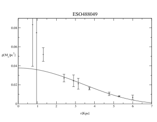
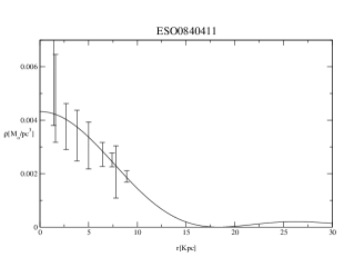
Figure 9: Density profile fits for the galaxies ESO1870510, ESO0488049, ESO0840411.

- (1) Alcubierre M., Guzmán, F. S., Matos, T., Núñez D., Ureña-López, L. A. and Wiederhold, P. 2002, Class. Quantum Grav. 19, 5017.
- (2) Alcubierre, M., Becerril, R., Guzmán, F. S., Matos, T., Núñez, D., and Ureña López, L. A., 2003, Class. Quantum Grav., 20, 2883
- (3) Arbey, A., Lesgourgues, J. and Salati, P. 2001, Phys. Rev. D 64, 123528.
- (4) Arbey, A., Lesgourgues, J., and Salati, P., 2001, Phys. Rev. D65, 083514 (2002).
- (5) Böhmer C. G. and Harko, T., E-print astro-ph/0705.4158
- (6) Guzmán, F. S., and Matos, T., 2000, Class. Quantum Grav. 17, L9.
- (7) Guzmán, F. S. and Ureña-López, L. A. 2003, Phys. Rev. D 68, 024023.
- (8) Guzmán, F.S., & Ureña-López, L.A. 2004, Phys. Rev. D 69, 124033.
- (9) Guzmán, Francisco Siddhartha and Ureña-López, L 2005, In ”Progress in Dark Matter, Ed. Nova Science”
- (10) Hawley, S. H., and Choptuik, M. W., 2000, Phys. Rev. D, 62, 104024
- (11) Honda, E. P., and Choptuik, M. W., 2001, E-print hep-ph/0110065.
- (12) Hu, W., Barkana, R., and Gruzinov, A., 2000, Phys. Rev. Lett., 85, 1158
- (13) Ji, S. U., and Sin, S. J., 1994, Phys. Rev. D, 50, 3655
- (14) Lee, J. W., and Koh, I. G., 1996, Phys. Rev. D, 53, 2236
- (15) Lieu, R. E-print astro-ph/0705.2462.
- (16) MacGaugh, S. S., Rubin, V. C., and de Blok, W. J. G., 2001, ApJ, 122, 2381
- (17) Matos, T., and Guzmán, F. S., 2000, Ann. Phys. (Leipzig), 9, SI-133
- (18) Matos, T., Guzmán, F. S., and Núñez, D., 2000, Phys. Rev. D, 62, 061301
- (19) Matos, T., and Guzmán, F. S., 2001, Class. Quantum Grav., 18, 5055
- (20) Matos, T., & Guzmán, F.S. 2000, Annalen Phys. 9, S1-S133.
- (21) Matos, T. and Ureña-López, L. A. 2000, Class. quantum Grav. 17, L75.
- (22) Matos, T. and Ureña-López, L. A. 2001, Phys. Rev. D 63, 063506.
- (23) Peebles, P. J. E., 2000, E-print astro-ph/0002495.
- (24) Sahni, V., and Wang, L., 2000, Phys. Rev. D, 62, 103517
- (25) Schunck, Franz E. 1998, astro-ph/9802258
- (26) Seidel, E., & Suen, W-M. 1990, Phys. Rev. D 42, 384.
- (27) Seidel, E., and Suen, W., 1991, Phys. Rev. Lett., 66, 1659
- (28) Seidel, E., and Suen, W., 1994, Phys. Rev. Lett., 72, 2516
- (29) Sin, S. J., 1994, Phys. Rev. D, 50, 3650
- (30) Trott, C. M., and Webster, R. L., 2002 E-print astro-ph/0203196
- (31) Ureña-López, L. A. 2002, Class. Quantum Grav.19, 2617.144
- (32) Ureña-López, L. A., Matos, T. and Becerril, R. 2002, Class. Quantum Grav. 19, 6259.