The Composition Gradient in M101 Revisited. II. Electron Temperatures and Implications for the Nebular Abundance Scale

Abstract

We use high signal/noise spectra of 20 H II regions in the giant spiral galaxy M101 to derive electron temperatures for the H II regions and robust metal abundances over radii R = 0.19–1.25 R₀ (6–41 kpc). We compare the consistency of electron temperatures measured from the [O III]$\lambda$4363, [N II]$\lambda$5755, [S III]$\lambda$6312, and [O II]$\lambda$7325 auroral lines. Temperatures from [O III], [S III], and [N II] are correlated with relative offsets that are consistent with expectations from nebular photoionization models. However, the temperatures derived from the [O II]$\lambda$7325 line show a large scatter and are nearly uncorrelated with temperatures derived from other ions. We tentatively attribute this result to observational and physical effects, which may introduce large random and systematic errors into abundances derived solely from [O II] temperatures. Our derived oxygen abundances are well fitted by an exponential distribution over six disk scale lengths, from approximately 1.3 (O/H)_⊙ in the center to 1/15 (O/H)_⊙ in the outermost region studied (for solar 12 + log (O/H) = 8.7). We measure significant radial gradients in N/O and He/H abundance ratios, but relatively constant S/O and Ar/O. Our results are in approximate agreement with previously published abundances studies of M101 based on temperature measurements of a few H II regions. However our abundances are systematically lower by 0.2–0.5 dex than those derived from the most widely used strong-line “empirical” abundance indicators, again consistent with previous studies based on smaller H II region samples. Independent measurements of the Galactic interstellar oxygen abundance from ultraviolet absorption lines are in good agreement with the $T_{e}$-based nebular abundances. We suspect that most of the disagreement with the strong-line abundances arises from uncertainties in the nebular models that are used to calibrate the “empirical” scale, and that strong-line abundances derived for H II regions and emission-line galaxies are as much as a factor of two higher than the actual oxygen abundances. However other explanations, such as the effects of temperature fluctuations on the auroral line based abundances cannot be completely ruled out. These results point to the need for direct abundance determinations of a larger sample of extragalactic H II regions, especially for objects more metal-rich than solar.

1 INTRODUCTION

The spiral galaxy M101 (NGC 5457) has played a central role in our understanding of gas-phase abundance distributions in galaxies. Its large disk ($R_{0}$ = 14.4 arcmin = 32.4 kpc; de Vaucouleurs et al. 1991) contains well over 1000 catalogued H II regions (Hodge et al. 1990; Scowen, Dufour, & Hester 1992) with a large radial range in excitations and metal abundances. Spectrophotometry of its brightest H II regions by Searle (1971) and Smith (1975) provided some of the first quantitative measurements of radial abundance gradients in disks.

The first systematic studies of H II region abundances in galaxies were based on “direct” methods, in which measurements of temperature-sensitive auroral lines (usually [O III]$\lambda$4363) were used to constrain the temperature and emissivities of the abundance-sensitive forbidden lines directly. M101 was the object of several such studies, each based on electron temperature ($T_{e}$) measurements of 1–5 bright H II regions (Searle 1971; Smith 1975; Shields & Searle 1978; Rosa 1981; Sedwick & Aller 1981; Rayo, Peimbert, & Torres-Peimbert 1982; Torres-Peimbert, Peimbert, & Fierro 1989; Kinkel & Rosa 1994; Garnett & Kennicutt 1994). These studies established the existence of a roughly exponential abundance gradient in the disk, and with roughly a fivefold range in abundance over the range of radii studied ($\sim$0.2–0.8 $R_{0}$). They also established that the pronounced nebular excitation variations observed among extragalactic H II regions are driven primarily by changes in their electron temperatures. For compositions typical of present-day disks the dominant ionized gas coolants are fine-structure lines of heavy elements, so the average electron temperature of an H II region decreases with increasing metal abundance.

The application of this “direct” abundance technique has been hampered by several technical limitations, however. For oxygen abundances much above $\sim$0.5 (O/H)_⊙, increased cooling by IR fine-structure lines causes the [O III]$\lambda$4363 line to become increasingly weak and difficult to detect, rendering direct abundance determinations based on this feature impossible. Questions about the linearity of photon-counting detectors used prior to the 1990s also reduced confidence in the abundances even when the [O III]$\lambda$4363 line was detected (e.g., Torres-Peimbert et al. 1989). Moreover, the [O III] temperature itself may not be a representative measure of the average temperature in regions where O⁺⁺ occupies a small fraction of the nebular volume or have significant internal gradients in $T_{e}$ (e.g., Stasińska 1978; Garnett 1992; Oey & Kennicutt 1993). Local fluctuations in electron temperature may also affect the temperature derived from integrated measurements of collisionally excited lines in the optical part of the spectrum (e.g., Peimbert 1967).

The absence of direct abundance measurements for metal-rich objects led to the development of “empirical” methods, in which the ratios of strong lines ([O II]$\lambda$3727, [O III]$\lambda\lambda$4959, 5007, [N II]$\lambda$6583, [S II]$\lambda\lambda$6717,6731, [S III]$\lambda\lambda$9069,9532) are used to estimate the oxygen abundance, without any direct electron temperature measurement (e.g., Pagel et al. 1979; Alloin et al. 1979; Edmunds & Pagel 1984; Dopita & Evans 1986; McGaugh 1991; Vílchez & Esteban 1996; van Zee et al. 1998; Dutil & Roy 1999; Díaz & Pérez-Montero 2000; Kewley & Dopita 2002). These methods rely on the physical coupling betweeen metal abundance and electron temperature, coupled with the observation of relatively tight correlations of forbidden-line ratios among extragalactic H II regions (e.g., Baldwin, Phillips, & Terlevich 1981; McCall, Rybski, & Shields 1985). Early applications of these empirical methods were calibrated using a combination of $T_{e}$-based abundances for metal-poor objects and nebular photoionization models at higher abundances (see Garnett 2003 for a review). However, most subsequent calibrations have relied increasingly on grids of H II region photoionization models (e.g., McGaugh 1991; Kewley & Dopita 2002).

Over the past 15–20 years the overwhelming majority of published abundance studies of spiral galaxies have been based on these strong-line methods. These have included several comprehensive studies of the abundance trends across large galaxy samples (e.g., McCall et al. 1985; Skillman, Kennicutt, & Hodge 1989; Vila-Costas & Edmunds 1992; Oey & Kennicutt 1993, Martin & Roy 1994; Zaritsky, Kennicutt, & Huchra 1994; Skillman et al. 1996; Pilyugin et al. 2002), and applications to the integrated spectra of high-redshift galaxies (e.g., Kobulnicky & Zaritsky 1999; Carollo & Lilly 2001; Kobulnicky et al. 2003). These methods have been applied to M101 by Scowen et al. (1992), Kennicutt & Garnett (1996, hereafter Paper I) and Pilyugin (2001b).

The widespread application of these “empirical” abundances has hardly lessened the need for a foundation of abundance measurements based on high-quality, robust electron-temperature measurements. Fortunately, the introduction of high-efficiency spectrographs with CCD detectors on 4–10 m class telescopes now makes such an undertaking possible, through measurements of other auroral lines such as [S III]$\lambda$6312, [N II]$\lambda$5755, and [O II]$\lambda\lambda$7320,7330 (e.g., Kinkel & Rosa 1994, Castellanos, Díaz, & Terlevich 2002 and references therein). The [S III]$\lambda$6312 line is an especially attractive thermometer, because it is observable to higher metal abundances than [O III]$\lambda$4363, and often samples a larger fraction of the nebular volume in these regions. Its chief disadvantage is the need for accurate spectrophotometry of the corresponding nebular lines of [S III]$\lambda\lambda$9069,9532 in the near-infrared, but with the advent of red-sensitive CCD detectors measurements of these lines are feasible (e.g., Garnett 1989; Bresolin, Kennicutt, & Garnett 1999 [hereafter BKG]; Castellanos et al. 2002).

This paper is the second in a series on the spectral properties and chemical abundances in M101. In Paper I we presented strong-line measurements of [O II], [O III], [N II], [SII], and [S III] for 41 H II regions, and used several empirical abundance calibrations to examine the radial and azimuthal form of the oxygen abundance distribution. In this paper we use higher quality spectra for 26 of these H II regions obtained with the MMT telescope to measure electron temperatures and temperature-based abundances. Our study is motivated by several goals:

i) To enlarge the sample of M101 H II regions with well-measured direct abundances (from 6 to 20), thereby enabling us to separate genuine radial trends in the abundances from local variations or other spurious effects.

ii) To extend by more than 50% the radial coverage of the abundance measurements, to 0.19–1.25 $R_{0}$.

iii) To take advantage of the large homogeneous data set and the large range of oxygen abundances in M101, to test for radial trends in N/O, S/O, Ar/O, and He/H abundance ratios, with improved sensitivity over most previous studies.

iv) To obtain robust CCD-based [O III] temperature measurements, without the systematic uncertainties introduced by detector nonlinearities in most of the previously published spectra.

v) To measure electron temperatures for two or more ions in a majority of the H II regions, which enables us to compare the temperature scales, test the reliability of the individual auroral lines, and test the relations between ionic temperatures that have been predicted by nebular models.

vi) To compare our temperature-based abundances with the published “empirical” strong-line calibrations, and with independent abundance constraints, in order to test the consistency of the respective scales and understand the physical origins of any systematic differences.

The remainder of this paper is organized as follows. In § 2 we describe the observations and data analysis procedures, and present the spectrophotometric data used in this analysis. In § 3 we use the data to derive electron temperatures and O, N, S, and Ne abundances, and discuss the consistency of the temperature scales. We analyze the radial abundance distributions in M101 themselves in § 4, and in § 5 we combine our new data with high-quality direct abundances from the literature, to compare the consistency of the direct and strong-line abundance scales. We conclude with a general discussion of the zeropoint and reliability of the extragalactic nebular abundance scale in § 6. To maintain consistency with Paper I we will adopt a distance to M101 of 7.5 Mpc (Kelson et al. 1995) throughout this paper. However, we now adopt the new solar oxygen abundance scale (12 + log (O/H)_⊙ = 8.70) following Allende Prieto et al. (2001) and Holweger (2001).

2 DATA

Table 1 lists the objects measured in this study. Following Paper I we have used the designations of Hodge et al. (1990) when available. Detailed information on the positions and alternate designations of these H II regions can be found in Paper I, and are not repeated here.

Our sample was selected to cover the maximum range in radius and abundance possible. For the outer disk ($R>0.3~{}R_{0}$) we measured most of the bright knots in the large complexes NGC 5447, 5455, 5461, 5462, and 5471, as well as other, isolated H II regions at intermediate radii. We also made an effort to obtain good azimuthal coverage, to avoid any bias that might be introduced by the possible asymmetry in abundance distributions in M101 (Paper I). Since we were aiming to detect at least one auroral line with high signal/noise, we concentrated on the brightest H II regions at any radius.

The metal-rich H II regions in the inner disk of M101 presented particular challenges. The low excitation of the H II regions in the inner disk makes detection of the auroral lines difficult, and the problem is exacerbated by the stronger stellar continua in most regions (i.e., lower emission-line equivalent widths; see Paper I) and the relative absence of bright H II regions. We obtained multiple integrations for 4 H II regions with $R<0.3~{}R_{0}$ (H972, H974, H1013, H336), but only the latter two objects yielded useful measurements of temperature-sensitive lines (§ 3.1).

In addition to H II regions from Paper I, we also observed the outermost H II region in the survey of Scowen et al. (1992) at (J2000) RA = 14^h 03^m 50$\fs$09, Dec = 54^∘ 38′ 05$\farcs$0, at a radial distance of 18′.0 (41 kpc) from the nucleus of M101. It is designated as SDH323 in Table 1 and the remainder of this paper. We also include in our analysis measurements of the outer disk H II region H681 from Garnett & Kennicutt (1994) made with the MMT Red Channel Spectrograph, and analyzed using the same procedures as described below.

2.1 Spectrophotometry

Most of the spectroscopic data used in this paper were obtained in 1994–1997 with the Blue Channel Spectrograph on the 4.5 m MMT Telescope. An additional spectrum of one object (H336 = Searle 5) was obtained in 2002 January using the same spectrograph on the upgraded 6.5 m MMT. In addition, fluxes of lines longward of 6800 Å were taken from data obtained on the MMT with the Red Channel Spectrograph, as described in Paper I.

Spectra covering the region 3650 – 7000 Å were obtained using a 500 grooves mm^-1 grating blazed at 5410 Å, used in first order with a 3600 Å cutoff blocking filter. A 2″$\times$ 180″ slit yielded a spectral resolution of 6 Å FWHM. The spectrograph was equipped with a 3072 $\times$ 1024 element thinned Loral CCD detector, providing a spatial scale of $0\farcs 6$ per (binned) pixel. H II regions were observed for 1–3 integrations of 1200 s each. This provided high signal/noise (S/N $\gg$ 50) measurements of the principle diagnostic emission lines and measurements of faint lines including [O III]$\lambda$4363 and [S III]$\lambda$6312 in all but the lowest-excitation H II regions.

For the low-excitation metal-rich H II regions, higher-resolution spectra were obtained to provide more sensitivity to the faint temperature-sensitive [S III]$\lambda$6312 and [O II]$\lambda\lambda$7320,7330 lines. H336 (Searle 5), H409 (NGC 5455), H1013, and H1105 (NGC 5461) were observed using a 1200 grooves mm^-1 grating blazed at 4830 Å, tuned to cover the wavelength range 6000 – 7500 Å with a resolution of 2.4 Å FWHM. Integration times ranged from 600 s for the NGC regions to 2400 s for the fainter and more metal-rich H336 and H1013. The flux scale of these spectra were tied to the full-coverage spectra described above at H$\alpha$.

For spectral lines longward of 7000 Å (mainly [O II]$\lambda$7320,7330 and [S III]$\lambda$9069,9532) we used echellette spectra obtained with the Red Channel Spectrograph on the MMT, as described in detail in Paper I. These spectra cover the wavelength range 4700 – 10000 Å, and were taken with a 2″$\times$ 20″ slit, yielding a spectral resolution of 7 $-$ 15 Å FWHM. The flux scales of the two sets of spectra were tied together at H$\alpha$.

Standard stars from the list of Massey et al. (1988) were observed several times per night to determine the flux calibration. Care was taken to orient the spectrograph slit with the atmospheric dispersion direction for all standard star measurements, and for the H II regions when the dispersion was significant. Standard dark, flatfield (including twilight sky measurements), and HeNeAr lamp exposures were taken to calibrate CCD sensitivity variations, camera distortions, and the wavelength zeropoint.

The spectra were reduced using the TWODSPEC package in the NOAO IRAF package, using standard procedures. Since more than one object sometimes was observed along the slit, the spectra were fully reduced and calibrated in two dimensions before extracting one-dimensional flux-calibrated spectra for each H II region. The size of the extraction aperture was adjusted depending on the size of the H II region (typically 6″ – 10″), and was matched to the aperture used in the Red Channel spectra from Paper I.

Line intensities were measured by integration of the flux under the line profiles between two continuum points identified on each side of the line. For partly overlapping lines (e.g., H$\alpha$+[N II]$\lambda\lambda 6563,6548,6583$ and [SII]$\lambda\lambda 6716,6731$) gaussian profiles have been assumed to deblend the different components. Average spectra were measured in those cases where multiple observations with the same grating were taken. When available, line fluxes from the higher resolution spectra were retained for the subsequent analysis, after a consistency check with the lower resolution spectra was carried out.

The accuracy of the spectrophotometry was checked in several ways, from consistency of the standard star calibrations on a given run (typically $\pm$2–3% rms over the entire wavelength range), comparison of multiple measurements of the same H II regions, and, in the case of the faint lines, by Poisson statistics. Uncertainties for individual line measurements are listed in Table 1.

The observed spectra were corrected for interstellar reddening using the Balmer emission line decrement and the interstellar reddening law of Cardelli, Clayton, & Mathis (1989). We corrected for underlying stellar Balmer absorption by determining iteratively the equivalent width of the underlying stellar absorption that provides consistent values of the extinction $c(H\beta)$ for all the lines considered (H$\alpha$ through H$\delta$). For the intrinsic Balmer line ratios we have assumed the theoretical Case B values of Hummer & Storey (1987) at the temperature determined from the auroral lines.

3 ELECTRON TEMPERATURES AND ABUNDANCES

Analysis of the spectra was performed using the five-level atom program of Shaw & Dufour (1995), as implemented in the IRAF package with the exception of [S III], where we used updated collision strengths from Tayal & Gupta (1999). These yield [S III] temperatures that are about 200 K cooler and S⁺² abundances that are approximately 0.1 dex higher than produced by the 5-level program. Inspection of the [SII]$\lambda\lambda$6717,6731 doublet ratios in our H II regions shows that most of the emitting gas is at low electron densities ($n_{e}\ll 100$ cm^-3), so collisional effects on the derived temperatures and abundances should be negligible for most of the measured lines (possible exceptions are discussed below).

3.1 Electron Temperatures

Electron temperatures were derived using four sets of auroral/nebular line intensity ratios: [O III]$\lambda$4363/[O III]$\lambda\lambda$4959,5007, [S III]$\lambda$6312/[S III]$\lambda\lambda$9069,9532, [N II]$\lambda$5755/[N II]$\lambda\lambda$6548,6583, and [O II]$\lambda\lambda$7319,7330/[O II]$\lambda\lambda$3726,3729. In many of the H II regions one or more of the auroral lines was too faint to yield a reliable temperature measurement. Care must be taken to exclude low signal/noise auroral line measurements, to avoid having the temperatures biased by incompleteness effects. We propagated the measured line flux errors directly into the $T_{e}$ determination, and in the subsequent abundance analysis we discarded any data for which $\sigma(T_{e})\geq 1000~{}K$ or 10% (whichever was larger). This left 20 H II regions with a $T_{e}$ measurement from at least one auroral line, 17 objects with at least two temperature measurements, and 14 regions with three measurements. Three regions originally in the sample, H203, H972 and H974, did not yield any reliable auroral line detection, and these objects were dropped from the remaining analysis. Table 2 lists the derived electron temperatures and uncertainties for the sample. For most objects the uncertainties in the $T_{e}$ values are in the range $\pm$200–700 K.

The availability of multiple $T_{e}$ measurements for a large sample of H II regions allows us to compare the consistency of the various ionic temperature scales. Photoionization models can be used to predict scaling relations between temperatures measured in different ions, and these are commonly used in abundance analyses when only a single temperature measurement (usually [O III]$\lambda$4363) is available. Garnett (1992) carried out an extensive analysis of ion-weighted temperatures over the abundance range of interest, and we can compare the actual temperature relationships with those predicted by his models.

Figure 1 compares the measured [O II], [S III], and [N II] temperatures with [O III] temperatures derived for the M101 H II regions in Table 2 (solid points). In order to enlarge the comparison and check the reliability of our results we also include data from a study of NGC 2403 by Garnett et al. (1997). These latter data are plotted as open points. The dashed lines show the scaling relations predicted by the photoionization models of Garnett (1992):

$$\rm T[S\thinspace III]=0.83\ T[O\thinspace III]+1700~{}K$$ (1)

$$\rm T[N\thinspace II]=T[O\thinspace II]=0.70\ T[O\thinspace III]+3000~{}K$$ (2)

The best correlation is between [O III] and [S III] temperatures (T[O III] and T[S III], respectively), as shown in the top panel of Figure 1. Apart from a few objects with large uncertainties in one or both auroral line measurements, the respective temperatures roughly follow the theoretically predicted relationship from Garnett (1992). A similar correlation was observed by Vermeij & van der Hulst (2002) for a sample of Magellanic Cloud H II regions, albeit with larger observational uncertainties than in this study. This correlation is reassuring, and may alleviate some of the concerns raised about the utility of [O III] temperatures in moderate-abundance H II regions (e.g., Stasińska 2002). Despite the different ionization thresholds for S⁺⁺ and O⁺⁺ (23 eV vs 35 eV, respectively), the ions yield consistent measurements of $T_{e}$ over the range of temperatures where both auroral lines can be observed. In particular there is no evidence for [O III] temperatures being systematically higher in the higher-abundance, lower-temperature H II regions, as might be expected from temperature fluctuation effects.

The comparison of [N II] and [O III] temperatures (middle panel in Fig. 1) is less clear, because only a few regions have measured [N II]$\lambda$5755 lines, and for most of them the T[N II] is uncertain ($\sigma(T_{e})>1000~{}K$). The four regions with the best-determined temperatures show good agreement with the expectations from the Garnett (1992) models, but more data are needed to draw any meaningful conclusions. The discrepant points with the unphysically high [NII] temperatures all have very large uncertainties, and are probably the result of the susceptibility to anomalously large $T_{e}$ values for marginally detected lines that was alluded to earlier.

The most surprising comparison is between [O II] and [O III] temperatures, as shown in the bottom panel of Fig. 1. Although there may be a hint of a correlation in the extremes of the temperature range (e.g., $T_{e}<9000$ K vs $T_{e}>13000$ K), for most objects the two temperatures are uncorrelated. In order to assure ourselves that this result was not an artifact of an error in our data (e.g., poorly determined reddening corrections), we compiled data from other sources (Peimbert, Torres-Peimbert, & Rayo 1978; Hawley 1978; Talent & Dufour 1979; Vermeij & van der Hulst 2002) and these data show a similar inconsistency in temperatures.

The source of this disagreement remains unresolved, but we can speculate on possible sources. First, the ${}^{2}P^{o}$ level that gives rise to the [O II]$\lambda\lambda$7319,7330 complex (actually a pair of doublets) can be populated by direct dielectronic recombination into that level, as well by radiative cascade (Rubin 1986). This mechanism also affects the [N II]$\lambda$5755 line and the [O II]$\lambda$3727 doublet as well, although to a lesser degree. The net effect is that the electron temperature derived from the [O II] line ratio can be overestimated if the recombination contribution is not accounted for. The magnitude of the recombination contribution increases with both temperature and the O⁺² abundance, and so is a greater problem for hotter nebulae with large O⁺² fractions. Liu et al. (2000) provide correction formulae for the recombination contributions to the [O II] and [N II] line intensities:

$${{I_{R}(7319+7320+7331+7332)}\over{I({\rm H\beta})}}=9.36\,(T/10^{4})^{0.44}\times{{\rm{O}}^{+2}\over{\rm{H}}^{+}},$$ (3)

where $I_{R}/I({\rm H\beta})$ is the intensity of the recombination contribution to the [O II] line relative to H$\beta$.

We have estimated the likely contribution of recombination to the [O II]$\lambda\lambda$7319,7330 feature, using the [O III] electron temperatures from Table 3 and O⁺²/H⁺ ratios computed in Table 4. We find recombination typically contributes $<$ 5% to the [O II] line flux, which corresponds to a temperature error of only $\sim$2–3%, or less than 400 K in our worst case. Hence it cannot be a significant contributor to the discrepancy observed here. Note that recombination into [O II] would be expected to scatter the derived [O II] temperatures to systematically higher values.

It should also be noted that the [O II] $\lambda$7325/$\lambda 3727$ ratio is much more severely affected by collisional de-excitation than other $T_{e}$-sensitive ratios. A simple five-level atom analysis shows that the derived T[O II] can differ by as much as 1,000-2,000 K when changing $n_{e}$ from 10 to 200 cm^-3. Although our [S II]$\lambda$6717/$\lambda$6731 line ratios typically are consistent with $n_{e}$ being in the low density limit, in practice the uncertainties in the [S II] ratios are such that the 3$\sigma$ upper limits are of the order 200-300 cm^-3, thus permitting a fairly considerable range in electron density.

Other physical origins for discrepant [O II] temperatures might include radiative transfer effects, such as part of the [O II] emission arising in shadowed regions preferentially ionized by the diffuse radiation field, or a significant contribution of the [O II] from shocked regions. Shocks may be a significant contributor when one considers the supersonic turbulence that typifies giant H II regions (e.g., Chu & Kennicutt 1994; Melnick, Tenorio-Tagle, & Terlevich 1995 and references therein).

Observational uncertainties undoubtedly contribute to the scatter in T[O II] as well. The large wavelength difference between the [O II] features (3727 – 7325 Å) makes their ratio more sensitive to uncertainties in interstellar reddening. This is compounded by the fact that the two features can not be observed in a single spectroscopic setting, because of second-order contamination. The $\lambda$7325 feature is located in a region of relatively strong OH airglow emission, and is in the middle of a telluric water vapor band as well. All these effects probably raise the uncertainty in the [O II] line ratio considerably over the formal uncertainty based on photon statistical fluctuations. It is difficult to estimate the contributions to the uncertainties from some of these effects, and it is likely that the formal uncertainties for T[O II] in Table 2 underestimate the true errors.

Until the origin of the discrepancy of [O II] temperatures with other ions is understood, abundances derived solely on the basis of T[O II] measurements should be treated with skepticism.

3.2 Ionic and Total Elemental Abundances

The very good correlation between T[S III] and T[O III] in Figure 1, and its consistency with the predicted relation from ionization models, led us to calculate ionic abundances using a three-zone model for the electron temperature structure of an H II region (Garnett 1992). In this model the [O III] temperature is used to characterize the highest-ionization zone (O⁺², Ne⁺²), [S III] temperatures are used to characterize the moderate-ionization zone (S⁺², Ar⁺²), and the [N II] and [O II] temperatures to characterize the low-ionization zone. However, in view of the problems apparent in the [O II] temperatures, we needed to adopt an alternative procedure for setting the temperature in the low-ionization region.

We have used the scaling relations between [O II], [S III], and [O III] temperatures from Garnett (1992) to reduce the uncertainties in the individual $T_{e}$ measurements, and to estimate one or more of the zone temperatures above when a direct $T_{e}$ measurement was not available (Garnett et al. 1997). Instead of applying the measured T[O III] directly, we used equation [1] to derive a second estimate of T[O III] and averaged the two values to set the temperature in the high-ionization zone. The same process was applied in reverse to set $T_{e}$ in the moderate-ionization zone. Although this procedure introduces some dependence between the temperatures in the high- and moderate-ionization zones, it is justified by the tight correlation in the top panel of Fig. 1, and it reduces the random error in the derived abundances without introducing any systematic errors. We used equations [1] and [2] to estimate the temperature in the low-ionization zone, unless a direct $T_{e}$ measurement was available from [N II]. Table 3 summarizes these adopted electron temperatures.

Of the 22 H II regions in Table 1 with auroral line measurements, 19 objects have sufficient quality temperature measurements to provide reliable abundances. Two regions (H237, H875) were excluded because only [O II] temperatures were measured, and one region (H140) was dropped because the remaining [S III] or [O III] temperatures were too poorly measured to provide accurate abundances measurements on their own. The addition of H681 from Garnett & Kennicutt (1994) leaves us with robust $T_{e}$-based abundances for 20 H II regions. Table 4 lists the ionic abundances for O⁺, O⁺², S⁺, S⁺², N⁺, Ne⁺², and Ar⁺² (all with respect to hydrogen), computed using the adopted electron temperatures in Table 3. Table 5 lists the total elemental abundances for O, N, S, and Ne.

The current data set is unique in that it provides a large number of $T_{e}$-based abundances for a spiral galaxy, over large ranges in metal abundance and nebular ionization. This enables us explore the behavior of the ionization (and the reliability of the commonly applied ionization corrections) for several heavy elements. We discuss helium separately in § 4.4.

For oxygen, we know from the weakness of He II $\lambda$4686 that a negligible fraction of the gas is in O⁺³, so the oxygen abundance is simply the sum (O⁺ + O⁺²). For nitrogen we made the usual assumption that N/O scales with N⁺/O⁺, although this has not yet been demonstrated to be generally applicable (Garnett 1990).

Sulfur requires a correction for unobserved S⁺³ in high-ionization regions. This is illustrated in Figure 2, where we show the ratio (S⁺ + S⁺²)/(O⁺ + O⁺²) vs the O⁺ fraction, for H II regions in M101 and other objects from Garnett (1989) and Garnett et al. (1997). The sharp drop in S⁺ + S⁺² relative to O in highly-ionized regions (i.e., low O⁺/O) is symptomatic of an increasing contribution from unobserved S⁺³. To account for the S⁺³ contribution we used the correction formula of Stasińska (1978) and French (1981):

$${{S^{+}+S^{+2}}\over S}=\biggl{[}1-\biggl{(}1-{O^{+}\over O}\biggr{)}^{\alpha}\biggr{]}^{1/\alpha},$$ (4)

using $\alpha$ = 2.5, which is consistent with the sulfur ionization trends derived from photoionization models by Garnett (1989). This relation is plotted as the solid curve in Figure 2, for an assumed (constant) intrinsic log (S/O) = $-$1.60. While this relation appears to adequately follow the data for O⁺ fractions greater than 0.2 (including most or all of the M101 H II regions in this paper), the objects with higher ionization appear to fall below the curve. This could indicate that the models underpredict the S⁺³ fraction in high-ionization nebulae. This remains to be explored through further modeling and observations of [S IV]$\lambda$10.5 $\mu$m. Observations of many Galactic and LMC H II regions with the Infrared Space Observatory (ISO) indeed show strong [S IV] emission (e.g., Peeters et al. 2002a, b; Martín-Hernandez et al. 2002).

Argon presents problems similar to those for sulfur, because three ionization states can be present in H II regions. Ar⁺ is present in low-ionization nebulae, while Ar⁺³ can appear in H II regions of the highest degree of ionization. The ionization potentials of sulfur and oxygen bracket the respective levels in argon, so we have tested whether the observed ionic ratios in O or S can be used to derive a useful ionization correction factor (ICF) for argon. Figure 3 (top panel) shows that Ar⁺²/O⁺² is a poor predictor of Ar/O, as this ion ratio is strongly correlated with O⁺/O over the entire range sampled by our H II regions. On the other hand a plot of Ar⁺²/S⁺² vs O⁺ fraction (bottom panel of Figure 3) shows very little correlation; only the lowest-ionization region (H336) shows any significant deviation from a constant Ar⁺²/S⁺². Our measurements of 15 H II regions in M101 (excluding H336) and 8 H II regions in NGC 2403 (Garnett et al. 1997) yield a mean log (Ar⁺²/S⁺²) = –0.60$\pm$0.05. Thus for the purposes of this study we will assume that Ar/S = Ar⁺²/S⁺².

Neon is observed mostly in high-ionization, low-abundance H II regions via the [Ne III] $\lambda$3869 line, and in those cases it is usually assumed that Ne⁺²/O⁺² = Ne/O. This line is rarely observed in metal-rich H II regions, however, so the ionization corrections are less well constrained. A further difficulty is that models for the ionization of neon are sensitive to the input stellar atmosphere fluxes, which are themselves sensitive to the treatment of opacity and stellar winds. For this reason ionization models have had difficulty reproducing [Ne III].

The determination of the form of an ICF for Ne requires infrared measurements of [Ne II] and [Ne III] lines along with optical measurements of [O II] and [O III]. Few such measurements exist over a large range of O⁺/O. We have examined recent results from ISO spectroscopy of H II regions in M33 by Willner & Nelson-Patel (2002) and in the Magellanic Clouds by Vermeij & van der Hulst (2002). Figure 4 shows Ne⁺²/Ne vs. O⁺/O for the regions in these studies having both optical and IR measurements. The data clearly indicate that Ne⁺²/Ne declines strongly as the O⁺ fraction increases. On the other hand, the observational scatter is significant, and there are too few measurements for low-ionization regions (O⁺/O $>$ 0.5) to reliably derive a functional form for the Ne ICF at this time. Figure 5 shows the Ne⁺²/O⁺² ratios for our M101 H II regions. The data are consistent with a constant ratio over a wide range of ionization, but the scatter increases considerably as O⁺/O increases. This is partly due to observational scatter, but probably also reflects greater sensitivity to the local radiation field as Ne⁺² and O⁺² become minor constituents. The data are consistent with a constant Ne/O abundance ratio in M101, but do not establish this unambiguously. In view of the uncertainty in the Ne ICFs we shall not discuss the neon abundances further in this paper.

4 The Abundance Gradient in M101

These new abundance measurements provide largest and most complete radial coverage of any galaxy measured to date. We first discuss the radial behavior of the overall heavy element abundance gradient (via O/H), and then examine the other heavy element and helium abundance properties.

4.1 Oxygen Abundances

Figure 6 shows the radial dependence of the oxygen abundances for the 20 H II regions in our sample with reliable $T_{e}$ measurements. The error bars show the uncertainty in abundance as propagated from errors in the line measurements; these are dominated by the auroral line measurements. For most of the H II regions in the sample, the choice of ionic temperature for the low-ionization zone has a small effect on the derived abundance ($\leq$0.05 dex). This is a reflection of the consistency of the [S III] and [O III] temperatures discussed earlier, combined with the milder dependence of abundance on $T_{e}$ for intermediate-abundance H II regions. However the choice of temperature is significant at the extremes of the abundance distribution, especially for the three innermost H II regions.

In terms of the revised solar value of 12 + log (O/H)_⊙ = 8.7, the gas-phase oxygen abundances in M101 range from 1.2 $\pm$ 0.2 (O/H)_⊙ in the center to 0.07 $\pm$ 0.01 (O/H)_⊙ at R = 41 kpc. The abundance in the outermost disk is comparable to that of all but the most extreme metal-poor dwarf irregular galaxies. For comparison I Zw 18, the most metal-poor H II galaxy known, has an abundance 12 + log (O/H) = 7.2 or 0.03 (O/H)_⊙ on the new solar scale.

Numerous other authors have measured $T_{e}$-based abundances for small samples of H II regions in M101, as compiled in Table 6. Figure 7 shows that our results are generally in good agreement with these previous measurements. The rms difference between our O/H values and those from the literature is 0.11 dex, or 0.09 dex if we exclude H336, the most discrepant point, and we see no large-scale systematic differences. As one might expect the differences are larger for the more metal-rich H II regions, which have lower and more difficult to measure temperatures. The abundances for these regions are very sensitive to the adopted $T_{e}$; for example in the innermost region H336 a difference in $T_{e}$ of only 600 K in T[O II] accounts for about 0.2 dex of the difference between our abundance and that of Kinkel & Rosa (1994). The rest comes from their use of an ionization model to derive O/H; if we use their measured $T_{e}$ values, we derive 12 + log (O/H) = 8.79.

The observed abundances are well fitted by an exponential distribution, as shown by the solid line in Figure 6. This line shows a least squares fit to the points, yielding:

$$\rm 12+\log\,(O/H)=8.76\,(\pm 0.06)-0.90\,(\pm 0.08)\,(R/R_{0}).$$ (5)

An independent $T_{e}$-based abundance measurement to H336 (Searle 5) is available from Kinkel & Rosa (1994). Those authors derived 12 + log (O/H) = 8.88 (no uncertainty quoted), which is significantly higher than our value of 8.55$\pm$0.16. Their measurement is plotted as an open circle in Figure 6, and the dashed line shows the resulting fitted exponential abundance distribution if we use their measurement instead of ours:

$$\rm 12+\log\,(O/H)=8.85\,(\pm 0.07)-1.02\,(\pm 0.10)\,(R/R_{0}).$$ (6)

The difference propagates to an uncertainty of $\pm$0.1 dex in the extrapolated central abundance At the adopted distance of M101 (7.5 Mpc), $R_{0}$ = 32.4 kpc, so the corresponding gradients from equations [5] and [6] are $-$0.029 and $-$0.032 dex kpc^-1 respectively. of M101 and $\pm$10% in the slope of the gradient. For a B-band disk scale length of 5.4 kpc (Okamura, Kanazawa, & Kodaira 1976), the corresponding gradient is $-$0.16 $\pm$ 0.01 dex per unit scale length.

The fact that the gradient in O/H remains closely exponential over six disk scale lengths is remarkable. There have been claims for a change in slope of the gradient in M101 at 0.3–0.5 $R_{0}$, based on strong-line estimates of O/H, and it has been argued that such a change could be related to the change in slope of the rotation curve (Scowen et al. 1992; Zaritsky 1992). More recently Henry & Howard (1995) and Pilyugin (2003) have argued that an exponential gradient was the best fit to the published data. Our results confirm that the purported changes in gradient slope are spurious and probably a result of systematic errors in the strong-line abundance estimators (§ 5). Claims of changes in the slope of abundance gradients based only on strong-line estimates should be regarded as uncertain.

Exponential heavy element abundance gradients have important consequences for chemical evolution models. A generic feature of chemical evolution models is that the composition gradients flatten with time, as a result of the breakdown of the instantaneous recycling approximation; as old, metal-poor stars die, they eject relatively metal-poor gas into the ISM at late times, and thus inhibit the enrichment of the ISM. This process proceeds more quickly in the dense inner regions of spirals, so that the models predict a flatter gradient in the inner disk than in the outer (e.g., Prantzos & Boissier 2000; Chiappini et al. 2002). However, such flattening of the gradients is rarely observed. This implies that some input assumption of the models is inadequate. Two possible explanations are that: (1) Disks are younger than assumed in the published chemical evolution models. In the models, the abundance gradients steepen with time early on, and then flatten from the inside out as the galaxy ages. In young disks the composition gradients are close to exponential. Thus if disks are younger than often assumed in the models (13-15 Gyr), then more uniform gradients would be expected. (2) Slow radial gas flows may redistribute gas and metals so as to maintain an exponential composition gradient. Lin & Pringle (1987) showed that viscous evolution of matter and angular momentum in disks can lead to exponential density distributions, while Clarke (1989) and Sommer-Larsen & Yoshii (1989) demonstrated that this can give rise to exponential composition gradients as well. It is as yet unclear how such radial gas flows can be maintained, or even what the magnitude of radial flows could be. Numerical simulations should help to address these questions (e.g., Churches, Nelson, & Edmunds 2001). If steep exponential abundance gradients are a common feature in disks this will need to be taken into account in galaxy evolution models.

Despite the well-defined exponential distribution, the points in Figure 6 show considerable scatter. Inspection of the data on a point-by-point basis shows that most or all of this scatter is due to uncertainties in the individual abundance measurements. For example, the scattering of points near $R/R_{0}$ = 0.42 and 0.53 are mainly different emission regions in the NGC 5462 and NGC 5447 complexes, respectively, which presumably have the same physical abundances. The rms residual between the data points and the fit is $\pm$0.09 dex, which is only marginally larger than the rms uncertainty of the individual measurements ($\pm$0.07 dex), and only one object (H128) deviates by more than 3$\sigma$ from the fitted gradient. As a result our data set is neither large enough nor accurate enough to test for local variations in abundances, such as the azimuthal asymmetry in nebular excitation and empirical abundance that was reported in Paper I.

4.2 N/O Abundance Ratios

Nitrogen shows a strong radial abundance gradient as well, and the behavior of the the differential N/O abundance ratio can place contraints on its nucleosynthetic origin.

Figure 8 shows the behavior of N/O with galactocentric radius (top panel) and as a function of oxygen abundance (bottom panel). There is a strong gradient in N/O across M101, as suspected from previous studies, and a significant correlation of N/O with overall O/H abundance. The two outermost H II regions in M101 have N/O values similar to those seen in dwarf irregular galaxies (e.g., Garnett 1990). The data in Figure 8 suggest a possible flattening of the N/O gradient in the outer parts of M101, consistent with the roughly constant value observed in dwarf galaxies, but we do not have enough data points to draw strong conclusions.

One region, NGC 5471-C, stands out as having a significantly higher N/O than expected. This is not an artifact of the data, as we saw relatively strong [N II] in our spectrum of this position from Paper I, and a similar enhancement was seen in observations of the region by Skillman (1985). NGC 5471 is known to contain a luminous supernova remnant at the position of NGC 5471-B (Skillman 1985; Chu & Kennicutt 1994; Chen et al. 2002), which can enhance the [N II] and [S II] lines. High resolution H$\alpha$ and [S II] images of NGC 5471 from HST do not show any anomalous structure in NGC 5471-C (Chen et al. 2002), but echelle observations by Chu & Kennicutt (1986) do reveal a region of high-velocity gas located within 0$\farcs$3 of the object. These fast-expanding regions often are associated with supernova remnants (e.g., Chu & Kennicutt 1994). Another possibility is a selective enhancement of nitrogen by the presence of Wolf-Rayet stars (Kobulnicky et al. 1997).

There is some debate over the existence of an N/O gradient within the Milky Way disk, with optical measurements giving relatively shallow N/O gradients while infrared studies show steeper gradients (cf. Shaver et al. 1983 vs Lester et al. 1987). It is not clear whether this discrepancy is due to ionization effects or observational errors (Garnett 1990). But the N/O gradient in M101 is unmistakable (Fig. 8), even without infrared measurements.

It is also instructive to compare the behavior of the N/O abundances in M101 with expectations from chemical evolution models. In the simple instantaneous chemical evolution model (Pagel 1997), ‘primary’ elements (i.e., those that are the ultimate product of the original H and He in a star at birth), are expected to vary in lockstep. A ‘secondary’ element (i.e., one produced from a heavy element seed present in the star at birth), on the other hand, is expected to grow in proportion to the abundance of primary elements. The solid line in the bottom panel of Figure 8 shows a simple model which includes a component with constant log (N/O) = –1.5, representing primary nitrogen, and a component for which log (N/O) = log (O/H) + 2.2, representing secondary nitrogen production. This simple representation provides an adequate description of the M101 data.

For comparison the dashed line in Fig. 8 shows a numerical one-zone model for the evolution of N/O vs. O/H from Henry, Edmunds, & Köppen (2000; hereafter HEK00). The line corresponds to their “best” Model B, which best reproduces the trend of N/O vs O/H in the data set they compiled for the study. Surprisingly, this model fails to reproduce our M101 results; the predicted N/O is too low at intermediate abundance (log O/H = 8.2 to 8.6), and rises too steeply at high abundance. Comparison with their other Models A and C (with lower and higher star formation efficiencies, respectively) does not alter this conclusion. We suspect that this discrepancy is mainly due to the oxygen abundance scale adopted by HEK00. Their data for spirals consisted largely of H II regions with abundances derived from strong-line calibrations, which yield systematically higher O/H than $T_{e}$-based abundance measurements (§5). In contrast, N/O is only modestly affected by the different abundance determination methods, because of its much weaker dependence on electron temperature. The result is that we observe N/O to increase more steeply at intermediate O/H than the HEK00 models. This example illustrates the critical importance of robust abundance measurements of extragalactic H II regions, and of establishing the normalization of the nebular abundance scale, for modeling and understanding the chemical evolution of galaxies.

On the basis of their models, HEK00 suggested that the secondary component of nitrogen in spiral disks arises mainly from processing of carbon, that is, mainly from CN cycling in intermediate mass stars. On the other hand, our M101 data suggest that nitrogen enhancement (relative to oxygen) is inititated at much lower metal abundances than in the HEK00 models. The fact that we can reproduce the trend in N/O with a component that grows proportionately with O/H suggests that secondary nitrogen is produced mainly from oxygen, and implies that the main source is full CNO cycling in massive stars. A comparison of the variation of nitrogen with carbon and oxygen abundances would be very informative in this regard, but this awaits the acquistion of much more data on carbon abundances in galaxies.

4.3 S/O and Ar/O Abundance Ratios

Elementary nucleosynthesis theory predicts a common primary origin for oxygen, sulfur, and argon in the cores of massive stars, so one would expect much less systematic variation in the S/O and Ar/O abundance ratios. Figure 9 shows the behavior of S/O and Ar/O in M101 (where Ar/O is derived from Ar/S and S/O, as discussed in § 4.2). Excluding the lower limit for the outermost region (SDH 323), we see no dependence of S/O on absolute abundance. The two most metal-rich regions in our sample do appear to have systematically smaller Ar/O than the bulk of the sample, and it is not clear whether the low values might be the result of observational errors or uncertainties in the ionization correction. The dashed lines in Figure 9 show the average S/O and Ar/O ratios for H II regions in dwarf irregular galaxies (as compiled by Izotov & Thuan 1999). Our results are consistent with the extrapolation of these trends, although our average S/O appears to be slightly smaller (and our average Ar/O slightly larger) than those reported by Izotov & Thuan.

Observations of M51 by Díaz et al. (1991) suggest evidence for a lower S/O ratio in very metal-rich H II regions. We do not see any of a similar decline in S/O in the inner disk of M101, but our measurements do not extend to as high metallicities as in M51. On the other hand, we do see hints of a lower Ar/O at high metallicity in M101. It should be noted that if the electron temperatures are higher in the M51 regions than those predicted by the photoionization models (§5), then Díaz et al. (1991) would have derived higher S/O ratios. A decrease in S/O and Ar/O in metal-rich environments would be of considerable interest, as it would indicate some dependence of stellar nucleosynthesis or the stellar initial mass function with metallicity.

4.4 Helium Abundances

The large abundance range in our data set allows us to test for a systematic change in the helium abundance with metallicity. Although our data were not taken for this purpose, we have high $S/N$ measurements of several He I lines for many of the H II regions, as summarized in Table 7. Listed are the He I line strengths (relative to H$\beta$), along with the corresponding uncertainties and equivalent widths (EWs). The He I lines are influenced by underlying stellar absorption, and this will introduce spurious gradients in the derived He abundances if corrections for the absorption are not applied. Olofsson (1995) computed equivalent widths of stellar H I and He I lines for OB star associations; however, these calculations do not include He I from B stars. This is unfortunate since the He I EWs in stars are a maximum at spectral type B0. González-Delgado, Leitherer, & Heckman (1999) model starbursts consistently over a wide range of ages, but provide He I EWs only for lines blueward of 5000 Å. Self-consistent calculations of H I and He I EWs for OB associations for the stronger red He I lines are needed to estimate corrections for He abundances in H II regions. This is especially important at low metallicities for the primordial He problem (e.g., Olive, Skillman, & Steigman 1997; Izotov & Thuan 1999).

We derived approximate corrections for He I absorption based on direct measurements of He I EWs for stars by Conti & Altschuler (1971), and Conti (1973, 1974), which provide a comprehensive compilation of He EWs as a function of spectral type for O stars. Guided by the results of González-Delgado et al. (1999) for the He I $\lambda$4026 and $\lambda$4471 lines in 2-3 Myr old starbursts, we assumed a luminosity-weighted average spectral type of O7 for our M101 regions and obtain estimated EWs of 0.5 Å for $\lambda$4026, 0.5 Å for $\lambda$4471, 0.8 Å for $\lambda$5876, and 0.3 Å for $\lambda$6678. In computing He abundances we used the He I emissivities of Benjamin et al. (1999). Correcting our He I emission line strengths for these absorption EWs yields much better agreement between the He⁺ abundances computed from different lines. The He⁺ abundances computed from each measured He I line are listed in Table 8, along with the weighted average for all measured He I lines in each H II region. Note that the He⁺ abundances for the outermost region SDH 23 differ considerably for the 4471 and 5876 Å lines; the 5876 Å line is affected by a cosmic ray, and so we adopt the value derived from $\lambda$4471 as the He⁺ abundance for this object.

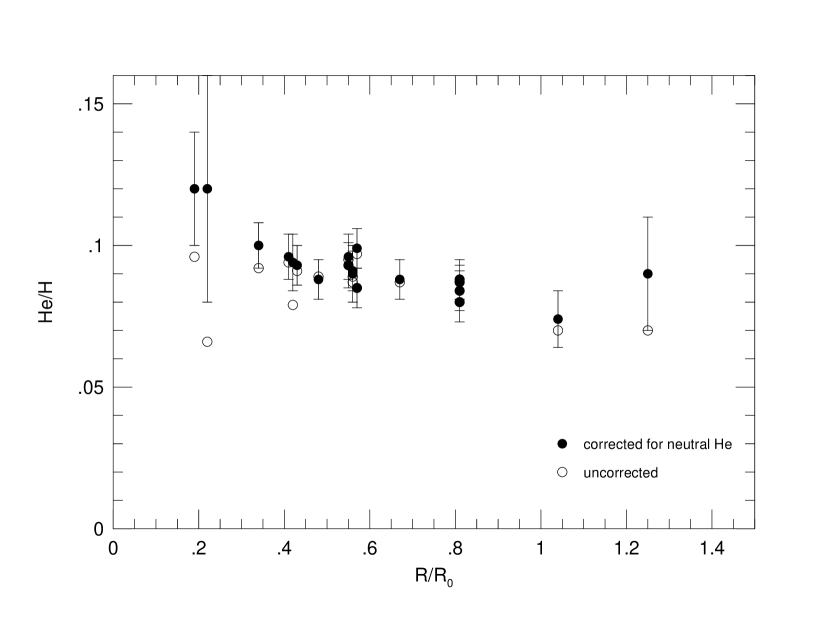
Figure 10: Helium abundances in M101 plotted as a function of galactocentric radius. The open circles show the uncorrected ionized He⁺/H⁺ ratios, while the filled circles show the total He abundances, corrected for neutral helium as described in the text.

The final correction in our derivation of He/H is accounting for neutral He, which is not directly observable in the ionized region. As shown in Figure 10 (open circles), the derived He⁺/H⁺ abundance ratio declines in the metal-rich inner disks of M101 and other spiral galaxies (also see BKG). This is probably due to the presence of cooler ionizing stars and low ionization in these H II regions (BKG). We estimated ionization correction factors for He using the ionization models of Stasińska (1990). The He⁺ fraction is roughly correlated with O⁺/O, with the He⁺ fraction close to unity for O⁺/O $<$ 0.2, and He almost entirely neutral for O⁺/O $>$ 0.9. At intermediate values, however, the He⁺ fraction can vary considerably at fixed O⁺/O due to variations in ionization parameter, making the He ICF rather degenerate. This degeneracy can be broken if the ionization parameter can be constrained, for instance using the S⁺/S⁺² ratio. We therefore use our measured values of S⁺/S⁺² and O⁺/O to estimate more accurately the ICFs for He.

The resulting He abundances are plotted as a function of radius in Figure 10 (solid points), and as a function of O/H in Figure 11. Although the measurement uncertainties are substantial, the plots show the presence of a significant radial gradient in He/H, after the neutral He corrections are applied. Only the outermost region (SDH 323) shows much deviation from this gradient, but its measurement is very uncertain due to the lack of a [S III]$\lambda\lambda$9069,9532 measurement for this object. The trend suggests we have likely overestimated the ICF for SDH 323, but this should be confirmed by observations of [S III].

The solid and dashed curves in Figure 11 show fits by Olive et al. (1997) to He abundance measurements in two samples of metal-poor dwarf galaxies (their sets B and C, respectively; see their Table 1 for parameters of the fits). The M101 He abundances appear to extrapolate the dwarf galaxy trends very well. We can not yet clearly differentiate between the two fits, although our abundances appear to be more consistent with the shallower dependence on O/H. A larger set of precise He line measurements for metal-rich regions would provide better limits on the slope of the He/O relation, which is an important constraint on stellar nucleosynthesis and the effects of stellar mass loss on yields (Maeder 1992), as well as on the primordial He abundance.

5 Comparison with Empirical Abundance Scales

As discussed in §1, abundance estimates based on strong-line “empirical” methods have largely supplanted direct, $T_{e}$-based determinations for large-scale abundance surveys and cosmological lookback studies. With the large dynamic range in O/H in our data set, it is instructive to compare our direct abundances with those derived for the same H II regions using the most popular strong-line calibrations. In order to enlarge the comparison we have also included recent high-quality direct abundance measurements of H II regions in other galaxies from the literature (Garnett et al. 1997, van Zee et al. 1998; Deharveng et al. 2000; Díaz & Pérez-Montero 2000; Castellanos et al. 2002).

Figure 12 shows the well-known plot of oxygen abundance against the empirical abundance index $R_{23}$ (Pagel et al. 1979), where:

$$R_{23}\equiv{{(I([O\thinspace II]\lambda\lambda 3726,3729)+I([O\thinspace III]\lambda\lambda 4959,5007))}\over{I(H\beta)}}.$$ (7)

H II regions from this paper are plotted with solid points, while objects from the other papers cited above are indicated with open squares. The superimposed lines show examples of widely-used calibrations for $R_{23}$, as taken from the references indicated in each panel. These particular examples were selected to illustrate the range of $R_{23}$ calibrations in the literature. The $R_{23}$ index shows the well-known double-valued behavior, with oxygen line strength increasing monotonically with abundance at low metallicities, and decreasing at high metallicities, the latter reflecting the dominance of oxygen cooling over abundance in metal-rich regions. Since most of the H II regions observed in spiral galaxies have metallicities that place them on the “upper” branch of this diagram, we will restrict the discussion in this paper to that part of the strong-line calibration, roughly corresponding to $12+\log~{}(O/H)\geq 8.0$.

Although the measured H II region abundances trace a locus which is roughly consistent in shape with most of the empirical calibrations, there is a pronounced offset in abundance in most cases, as has been pointed out previously (see Stasińska 2002 and references therein). In all cases the empirical calibrations yield oxygen abundances that are systematically higher than the $T_{e}$-based abundances, by amounts ranging from 0.1 to 0.5 dex, depending on the calibration and the excitation range considered. The calibrations of Pilyugin (2000, 2001a) shown in the lower right panel of Figure 12 show a smaller offset, mainly because those calibrations are partly based on $T_{e}$-based abundances.

Similar discrepancies are seen in most of the other “empirical” abundance indices, as is illustrated in Figure 13. Here we directly compare the $T_{e}$-based abundances with those derived from several different empirical indices, all calibrated with a common grid of photoionization models (Kewley & Dopita 2002), so the different indices can be evaluated on the same basis. The symbols are the same as in Figure 12. As noted earlier, there is a systematic shift toward larger abundances in the empirical calibrations, ranging from 0.2 to 0.5 dex on average.

The discrepancies shown in Figures 12 and 13 can be traced to two main origins, an insufficient number of calibrating H II regions with accurate $T_{e}$-based abundances in the earliest calibrations, and a systematic offset between the nebular electron temperatures in the calibrating photoionization models and the observed forbidden-line temperatures, for a given strong-line spectrum (e.g., Stasińska 2000). Because of the exponential temperature dependence on the strengths of these collisionally-excited forbidden lines ($\propto\exp{-\chi/{kT}}$), an offset in $T_{e}$ will have the strongest effect on the shorter wavelength features at a given abundance. The better consistency of $S_{23}$ in Figure 13 can be attributed in part to the relatively low excitation of the [S III]$\lambda\lambda$9069,9532 lines that dominate this index; note that at higher abundances, where the characteristic electron temperatures are very low, even this index deviates significantly from the direct abundance determinations.

Figure 14 shows a comparison of direct abundances with empirical values derived using the “$P$ method” of Pilyugin (2001a). At intermediate abundances (12 + log (O/H) $\simeq$ 8.5) the two abundance scales are in approximate agreement, in part because the method is calibrated with direct abundance measurements in this region. However the $P$ method results break down for 12 + log (O/H) $\leq$ 8.4. As can be seen in Figure 12, these regions fall into the abundance range where most of the empirical indicators become multiple-valued or very sensitive to nebular ionization parameter. Most authors are aware of these limitations and restrict the application of the various empirical tracers to the abundance range for which they are valid (see Pilyugin 2001a; Kewley & Dopita 2002 for detailed discussions). However the comparison in Figure 14 illustrates a pitfall in this approach. The $P$ method as calibrated is supposedly only valid for 12 + log (O/H) $\geq$ 8.2 (Pilyugin 2001a), but in the absence of electron temperature measurements when does one know for sure that an H II region falls within the applicable abundance range? If the empirical abundances overestimate the actual abundances by a significant factor, they may be applied in regions for which the calibration is invalid.

6 DISCUSSION

The results in the previous section may have significant consequences for the nebular abundance scale as a whole. If the forbidden-line abundances are correct, it implies that most studies of galactic abundances (locally and at high redshift) based on “empirical” nebular calibrations have over-estimated the true absolute oxygen abundances by factors of 1.5–3, for $12+\log({\rm O/H})>8.2$ (about 1/3 Z/Z_⊙). Our results do not apply to the low-metallicity part of the abundance scale, so another net effect of this change would be to reduce the total range of nebular abundances observed in galaxies. This may have significant effects on the measured abundance gradient slopes in some galaxies, and on applications such as the metallicity dependence of the Cepheid period-luminosity relation (e.g., Kennicutt et al. 1998).

It is not completely clear whether the discrepancies in Figures 12 and 13 are the result of a systematic error in the $T_{e}$-based abundances, the model-based “empirical” abundances, or both. There are well-documented reasons for questioning the accuracy of both abundance scales (also see Peimbert 2002, Stasińska 2002, and references therein).

It has been argued for many years that directly measured electron temperatures and the corresponding abundances from collisionally-excited lines may have systematic errors due to temperature fluctuations (Peimbert 1967). Because of the exponential temperature dependences of forbidden line emissivities, their fluxes will tend to be weighted toward regions of higher temperature, and in the presence of significant $T_{e}$ fluctuations they will yield anomalously high $T_{e}$ measurements, and thus low abundances. The importance of this effect on the nebular abundance scale depends on the magnitude of the actual temperature fluctuations in extragalactic H II regions. Observational evidence for significant $T_{e}$ fluctuations has been contradictory. Early comparisons of T[O III] in the Orion nebula with the temperature derived from the Balmer continuum [T$(Ba_{c})$] revealed a large discrepancy, but this has not been confirmed by subsequent measurements with improved detectors (Liu et al.  1995a). Significant differences between T[O III] and T$(Ba_{c})$ are observed in planetary nebulae (Liu et al. 2001), but it is not clear whether the two temperatures should be the same, given temperature stratification in ionized nebulae (Stasińska 1978; Garnett 1992). Direct searches for small-scale temperature fluctuations using high resolution HST imaging of planetary nebulae have yet to reveal any significant variations (Rubin et al. 2002).

Measurements of recombination lines of heavy elements (O II, C II, N II) provide an independent means of measuring nebular abundances, and they tend to yield higher values than the corresponding forbidden lines, by a factor that varies considerably (Liu et al. 1995b, 2001; Garnett & Dinerstein 2002). Recently Esteban et al. (2002) reported measurements of the O II recombination lines in the M101 H II regions NGC 5461 (H1105) and NGC 5471. These yielded O⁺²/H abundances that are 0.34 dex and 0.15 dex higher than our forbidden-line abundances, respectively, and this is consistent with the trends observed in other H II regions and planetary nebulae. However in many objects the abundance discrepancies are so large that they can not be explained by temperature fluctuations. The real explanation is not yet clear; Liu et al. (2001) postulate the presence of cold, dense, H-poor knots which produce most of the enhanced recombination line emission, while Garnett & Dinerstein (2002) note that dielectronic recombination may play a significant role. Unfortunately dielectronic recombination rates are rather uncertain at present (Savin 2000).

A third concern is relevant to metal-rich H II regions. At high abundances, strong cooling by infrared fine-structure lines of [O III] and [N III] greatly depresses the electron temperature in the high-ionization zone of H II regions relative to the lower-ionization zones, leading to a strong temperature gradient (Stasińska 1978). Under these conditions, the measured electron temperature can be higher than the ion-weighted mean temperature for a given species, and the optical forbidden lines can be weighted toward the higher temperature zones, leading one to underestimate the true abundances. The temperature gradient mimics the effects of temperature fluctuations, and can introduce differences between the measured $T_{e}$ and the ion-weighted temperature of up to 2000 K (see Fig. 6b in Garnett 1992). The results are sensitive to ionization parameter (which affects the amount of O⁺², and density (which affects the cooling rate in the infrared lines through collisional quenching).

Despite these concerns, however, there are good reasons to believe that the forbidden lines give close to the correct abundances, at least for the range of O/H of interest here. Recent measurements of infrared forbidden lines (which have weak temperature dependences) in the spectra of planetary nebulae yield abundances that are in good agreement with those from optical forbidden lines, even where there is a large discrepancy with recombination line abundances (Liu et al. 2000, 2001). Likewise, measurements of radio recombination line temperatures of Galactic H II regions give results that are consistent with forbidden line measurements of the same objects (Shaver et al. 1983; Deharveng et al. 2000).

Additional support for the reliability of the forbidden-line abundance scale comes from independent measurements of the local interstellar O/H from Galactic H II regions and ultraviolet absorption line measurements of the diffuse ISM. A recent determination of the Galactic abundance gradient by Deharveng et al. (2000), based on [O III]$\lambda$4363 measurements for 6 H II regions with $R_{G}=6.6-14.8$ kpc, yields a local oxygen abundance 12 + log (O/H) = 8.48. This value is in excellent agreement with local diffuse abundances of 8.50$\pm$0.02, 8.48$\pm$0.03, and 8.54$\pm$0.01 derived from HST and FUSE spectroscopy of multiple local sightlines (Meyer, Jura, & Cardelli 1998; Moos et al. 2002). These values are also in reasonable accord with the solar abundance (8.7), assuming modest grain depletion factors.

If the discrepancies in Figures 12–13 are due to errors in the model-derived “empirical” abundances, then what might be the cause? The typical H II region model is spherically symmetric, with a uniform density of 100 (or 10) cm^-3 and a central point ionizing source. In reality, the density distribution in many giant H II regions is dominated by filamentary, shell-like structures, often with dispersed, multiple ionizing sources within the boundaries of the ionized gas (e.g., Kennicutt 1984). In moderate to high-abundance H II regions the cooling is dominated by a few ions such as O⁺⁺, and this introduces a physical coupling between the thermal and ionization structures, which in turn can be influenced by the detailed distributions of gas and ionizing sources.

Unfortunately there are relatively few direct measurements of the electron density distributions, or even the characteristic densities in these regions. Density measurements from the [S II]$\lambda\lambda$6717,6731 line ratios generally lie at the low density limit, indicating $N_{e}<200$ cm^-3. Corroborating density measurements from other diagnostic ratios such as [O II]$\lambda\lambda$3726,3729 are rare. Accurate knowledge of the gas densities are particular important for metal-rich regions, because of the dramatic effect of collisional quenching on fine-structure cooling and the thermal structure of the nebulae (Oey & Kennicutt 1993).

The geometry of the ionizing sources within this complex structure may also influence the emergent spectra. The ionizing star clusters in some regions are centrally concentrated (e.g., 30 Doradus in the LMC, NGC 5461 in M101), but in others (e.g., NGC 604 in M33, I Zw 18), the ionizing stars are loosely distributed. Even in the 30 Doradus nebula, O3 stars are known to be located among the ionized filaments (Walborn 1991, Bosch et al. 1999). Since the ionization parameter depends in part on the distance of the ionizing source from the gas, an extended distribution of stars might be expected to affect the resulting nebular spectrum. Dust also affects the ionized gas, depleting Lyman-continuum photons, and by photoelectric heating and recombination cooling of the gas.

Finally, uncertainties in the input ionizing continua may play a role. Although the situation is improving here, with increasing use of non-LTE, spherical calculations which include realistic opacities and stellar winds, models for Lyman-continuum fluxes are still in the development stage. As shown by BKG and Bresolin & Kennicutt (2002), the improper treatment of the stellar ionizing flux, especially during the Wolf-Rayet phase, can lead to large discrepancies between observed H II spectra and those predicted by photoionization models based on synthetic spectral energy distributions. This situation is improving, thanks to advances in the codes describing massive star atmospheres. Recent stellar models (Martins, Schaerer, & Hillier 2002; Herrero, Puls, & Najarro 2002) show that the inclusion of mass loss and more realistic stellar opacities has an important effect on the effective temperature scale for O stars. Evolutionary models based on these new stellar atmospheres by Smith, Norris, & Crowther (2002) appear to be in good agreement with the ionization properties of extragalactic H II regions. Further study should determine if the directly measured and predicted H II region sequences are consistent.

In summary, we cannot be certain whether the discrepancies in abundance scales summarized in Figures 12–13 are due to biases in the $T_{e}$-based results, or problems in the theoretical models that are used to calibrate most of the strong-line “empirical” abundance scales. High-quality far-infrared measurements of a sample of extragalactic HII regions, including some of the principal fine-structure cooling lines, may help to resolve these inconsistencies. In the meantime it is important for users of the various abundance calibration methods to be aware of this discrepancy, and until it is resolved users should beware of combining strong-line abundance estimates with direct abundance measurements.

An accurate extragalactic metallicity scale is fundamental for constraining models of chemical enrichment, the chemical evolution of galaxies, and the cosmic baryon cycle. In this context it is sobering to recognize that there is a systematic uncertainty of a factor 2–3 in the zeropoints of one or more of the metal abundance calibrations. A few specific observational and theoretical investigations would go far toward resolving this problem. High signal/noise spectroscopy and electron temperature measurements for other extragalactic H II regions, especially metal-rich objects, would nail down the $T_{e}$-based abundance scale across the full O/H range, and help to quantify the disagreement between observations and ionization models across the full spectrum of abundances, densities, and ionization properties. Measurements of multiple auroral lines in the same objects (e.g., Fig. 1) would be especially valuable for reducing systematic errors in the $T_{e}$-based abundances, testing the reliability of specific nebular thermometers, and comparing with the predictions of the nebular models. Independent temperature and abundance measurements for H II regions, and extension of the wavelength coverage to the mid- and far-infrared emission lines would also help. And comparisons with young stellar abundances will provide independent constraints on the metallicity zeropoints (e.g., Venn et al. 2000; Trundle et al. 2002). On the theoretical side, explorations of the effects of nebular geometry, structure, and ionizing spectrum on the thermal structure of H II regions would be useful, along with targeted studies of specific transitions such as the [O II] thermometer (§3.1). Solving the abundance zeropoint problem is important not only for the observations of metallicities of galaxies, but also for validating our theoretical modeling and understanding of photoionized regions in galaxies.

Figure 1: The correlations between various emission-line electron temperature diagnostics. Filled symbols show our measurements for M101 H II regions; open symbols show measurements for H II regions in NGC 2403 from Garnett et al. (1997). The dashed line shows the predicted correlations from Garnett (1992) based on photoionization model calculations.

Figure 2: The ion ratio (S⁺ + S⁺²)/(O⁺ + O⁺²) as a function of oxygen ionization (O⁺/O) for our M101 H II regions (filled squares). Also plotted are data for NGC 2403 H II regions (open squares; Garnett et al. 1997), and for dwarf irregular galaxies (stars; Garnett 1989). The curve represents the sulfur ionization correction formula, equation [4], assuming an intrinsic abundance ratio log (S/O) = $-1.6$.

Figure 3: Two comparisons showing the relative ionization behaviors of Ar, O, and S in extragalactic H II regions. Top: Ar⁺²/O⁺² vs. O⁺ ionic fraction. Bottom: Ar⁺²/S⁺² vs. O⁺ ionic fraction. Symbols are the same as in Figures 2 and 5. Except for H336 with O⁺/O = 0.85, Ar⁺²/S⁺² shows little correlation with ionization, in contrast to Ar⁺²/O⁺².

Figure 4: The Ne⁺² ionic fraction as a function of O⁺ ion fraction, derived from optical and infrared spectroscopy of H II regions. Open circles are LMC and SMC regions from Vermeij & van der Hulst (2002). Filled squares are M33 H II regions from Willner & Nelson-Patel (2002).

Figure 5: The Ne⁺²/O⁺² ion abundance ratio for H II regions in M101 (filled squares) plotted as a function of O⁺ fraction. Symbols are the same as in Figure 2.

Figure 6: The oxygen abundance gradient in M101 from our 20 H II regions with electron temperature measurements. The linear fit to the data given by equation [5] is shown by the solid line. The open circle is the abundance for H336 obtained by Kinkel & Rosa (1994). The dashed line shows the resulting fit if we use this point instead of our measurement, as given by equation [6].

Figure 7: Comparison of our O/H abundance measurements for M101 H II regions with those from the literature. Data are given in Table 6.

Figure 8: Top: Radial variation of N/O for our M101 H II region sample. Bottom: N/O vs. oxygen abundance. The open circle shows the abundances derived by Kinkel & Rosa (1994) for H336. The solid curve is a simple model for N/O which has a constant primary component with log (N/O) = $-1.5$ and a secondary component in which N/O increases proportionally with O/H. The dashed curve shows model B from Henry et al. (2000), as discussed in the text.

Figure 9: Dependences of S/O (Top) and Ar/O (Bottom) on oxygen abudance in M101. The dashed lines show the average values for dwarf irregular galaxies as derived by Izotov & Thuan (1999).

Figure 11: Helium abundances in M101 as a function of oxygen abundance. The solid and dashed lines represent two relations derived from measurements of metal-poor dwarf galaxies by Olive, Skillman, & Steigman (1998).

Figure 12: Comparisons of different ’strong-line’ empirical abundance calibrations from the literature (dotted lines) with ’direct’ abundance determinations in the $\log R_{23}$ vs logarithmic oxygen abundance plane. Each panel contains the same data points; solid circles denote M101 H II regions from this paper, and open squares show published measurements of other, mostly metal-rich regions (see text for references). The dashed lines in each panel show a different $R_{23}$ calibration from the reference indicated. The Kobulnicky et al. (1999) and Pilyugin (2000, 2001) calibrations are parameterized in terms of $R_{23}$ and a secondary measure of the hardness of the radiation field ($y$ and $P$, respectively), and we have drawn curves which bracket the typical values encountered in the H II region samples.

Figure 13: Comparison of electron temperature based abundances (O/H)_Te with those derived from different strong-line calibrations. Full circles represent our M101 data, while crosses are used for metal-rich H II regions from Castellanos et al. (2002) and Díaz et al. (2000). The four panels show empirical abundances using the calibrations of Kewley & Dopita (2002) for $R_{23}$ (eq. [7]), [N II]$\lambda$6584/[O II]$\lambda\lambda$3726,3729, $S_{23}\equiv{([\rm S\thinspace II]\lambda\lambda 6717,6731+[S\thinspace III]\lambda\lambda 9069,9532)}$/$H\beta$, and a combined index, as described in their paper. For the $S_{23}$ comparison we have also compared to the original Díaz & Pérez-Montero (2000) calibration (open symbols).

Figure 14: Comparison of $T_{e}$-based abundances from this paper with those derived using the Pilyugin (2001b) $P$-method, as described in the text.

Table 1: Dereddened Line Fluxes and Errors

ID	[O II]		[Ne III]		[O III]		[O III]		[N II]		[S III]		[N II]		[S II]		[S II]		[Ar III]		[O II]		[S III]
	3727		3869		4363		5007		5755		6312		6584		6717		6731		7135		7325		9069+9532
H1013	188	10	3.0	0.2	$\cdots$	$\cdots$	103	5	0.5	0.1	0.8	0.1	64.6	3.4	16.7	0.9	12.1	0.6	7.8	0.5	2.6	0.3	131.6	7.0
H1105	185	10	18.3	1.0	1.4	0.1	316	17	0.4	$\cdots$	1.3	0.1	33.4	1.8	13.1	0.7	11.0	0.6	10.2	0.6	3.6	0.3	126.1	6.1
H1159	198	10	20.1	1.2	1.9	0.4	317	17	$\cdots$	$\cdots$	1.6	0.2	23.6	1.3	17.6	0.9	12.2	0.7	9.1	0.7	4.8	0.6	97.0	5.4
H1170	308	16	15.8	0.9	1.6	0.2	201	11	$\cdots$	$\cdots$	1.7	0.2	44.0	2.3	33.4	1.8	23.3	1.2	14.1	0.9	8.5	0.7	170.0	9.3
H1176	160	8	25.0	1.3	2.4	0.3	369	20	$\cdots$	$\cdots$	1.5	0.1	21.2	1.1	13.4	0.7	9.6	0.5	10.0	0.7	3.0	0.3	113.5	6.1
H1216	151	8	36.1	1.9	4.7	0.3	473	25	$\cdots$	$\cdots$	1.6	0.1	11.1	0.6	11.0	0.6	7.9	0.4	8.2	0.6	2.7	0.3	83.0	4.6
H128	145	8	24.5	1.3	1.7	0.2	391	28	0.3	$\cdots$	1.3	0.1	20.8	1.1	13.3	0.7	10.0	0.5	10.6	0.7	4.1	0.3	104.4	5.7
H140	317	17	10.0	1.2	$\cdots$	$\cdots$	114	6	$\cdots$	$\cdots$	1.9	1.5	60.2	3.4	48.3	3.1	32.6	2.3	5.2	1.0	9.1	1.2	75.3	6.0
H143	219	12	17.1	1.0	2.3	0.4	284	15	0.9	0.2	1.4	0.2	33.3	1.8	23.2	1.2	17.0	0.9	9.2	0.7	2.4	0.4	93.8	5.2
H149	212	11	18.4	1.0	1.8	0.4	318	17	0.9	0.2	1.4	0.1	35.9	1.9	21.1	1.1	16.1	0.8	11.6	0.8	5.6	0.4	95.4	5.0
H203	223	12	$\cdots$	$\cdots$	$\cdots$	$\cdots$	44	2	$\cdots$	$\cdots$	$\cdots$	$\cdots$	91.1	4.9	38.7	2.2	27.9	1.8	5.3	0.5	$\cdots$	$\cdots$	93.4	5.5
H237	136	8	5.0	0.9	$\cdots$	$\cdots$	114	6	3.2	1.3	$\cdots$	$\cdots$	48.3	2.7	21.1	1.6	14.2	1.3	8.1	0.7	5.1	0.8	69.4	4.3
H336	178	9	$\cdots$	$\cdots$	$\cdots$	$\cdots$	23	1	0.5	0.1	0.6	0.1	95.9	5.1	33.5	1.8	23.3	1.2	3.9	0.4	1.4	0.2	107.0	5.7
H409	218	12	24.6	1.3	2.3	0.2	370	20	0.4	0.1	1.7	0.1	27.3	1.4	17.2	0.9	14.0	0.7	9.2	0.7	4.7	0.4	90.1	4.9
H67	244	13	25.6	1.4	3.5	0.5	342	18	$\cdots$	$\cdots$	1.8	0.4	16.3	0.9	15.6	1.1	10.7	0.8	8.7	0.8	5.4	0.8	92.1	5.7
H70	311	16	23.6	1.4	2.5	0.5	267	14	$\cdots$	$\cdots$	1.4	0.2	23.6	1.3	26.5	1.4	20.7	1.1	$\cdots$	$\cdots$	$\cdots$	$\cdots$	$\cdots$	$\cdots$
H71	200	11	32.4	1.7	5.9	0.4	454	24	$\cdots$	$\cdots$	1.9	0.3	15.9	0.9	17.2	1.0	11.9	0.7	$\cdots$	$\cdots$	$\cdots$	$\cdots$	$\cdots$	$\cdots$
H875	283	15	$\cdots$	$\cdots$	$\cdots$	$\cdots$	102	5	$\cdots$	$\cdots$	$\cdots$	$\cdots$	64.1	3.4	36.4	1.9	26.3	1.4	6.5	0.6	3.6	0.4	75.3	4.8
H972	148	8	$\cdots$	$\cdots$	$\cdots$	$\cdots$	30	2	$\cdots$	$\cdots$	$\cdots$	$\cdots$	86.9	4.7	22.3	1.4	16.1	1.1	3.8	0.5	$\cdots$	$\cdots$	98.3	5.3
H974	166	10	$\cdots$	$\cdots$	$\cdots$	$\cdots$	28	3	$\cdots$	$\cdots$	$\cdots$	$\cdots$	73.6	4.9	33.1	3.9	23.5	3.6	$\cdots$	$\cdots$	$\cdots$	$\cdots$	37.6	11.8
N5471-A	106	6	52.2	2.8	9.5	0.5	644	34	$\cdots$	$\cdots$	1.6	0.1	6.8	0.4	8.7	0.5	7.1	0.4	7.7	0.6	3.8	0.3	61.4	3.4
N5471-B	213	11	35.4	1.9	6.6	0.4	395	21	0.4	0.1	1.3	0.1	16.7	0.9	29.1	1.5	25.6	1.3	6.4	0.4	8.6	0.6	50.9	3.1
N5471-C	174	9	34.4	1.8	5.4	0.3	416	22	1.2	0.1	1.4	0.1	25.1	1.3	13.1	0.7	10.1	0.5	6.8	0.5	5.2	0.4	65.9	3.7
N5471-D	137	7	48.4	2.6	8.0	0.4	578	31	$\cdots$	$\cdots$	1.7	0.1	8.5	0.5	11.7	0.6	8.9	0.5	8.0	0.6	1.8	0.3	75.7	4.3
SDH 323	194	10	28.0	1.7	5.5	0.9	227	12	$\cdots$	$\cdots$	$\cdots$	$\cdots$	7.9	0.7	12.0	1.0	8.8	1.0	$\cdots$	$\cdots$	$\cdots$	$\cdots$	$\cdots$	$\cdots$

Table 2: Measured Electron Temperatures (K)

ID	T[O II]		T[N II]		T[S III]		T[O III]
H1013	9000	400	8100	300	7200	200	$\cdots$	$\cdots$
H1105	9300	400	9400	400	8500	200	8900	200
H1159	8100	400	$\cdots$	$\cdots$	10200	500	9800	600
H1170	8600	300	$\cdots$	$\cdots$	8500	300	10800	400
H1176	10500	600	$\cdots$	$\cdots$	9300	300	10000	300
H1216	10300	600	$\cdots$	$\cdots$	11000	400	11500	200
H128	13000	800	10700	600	9200	200	8900	300
H143	8100	600	14100	2200	9800	600	10800	700
H149	12100	600	13600	1300	9800	300	9600	600
H336	7200	300	7300	400	7000	500	$\cdots$	$\cdots$
H409	10100	500	9900	1000	10900	300	10000	200
H67	7800	500	$\cdots$	$\cdots$	11100	1300	11600	600
H70	$\cdots$	$\cdots$	$\cdots$	$\cdots$	$\cdots$	$\cdots$	11300	800
H71	$\cdots$	$\cdots$	$\cdots$	$\cdots$	$\cdots$	$\cdots$	12700	400
N5471-A	13800	800	$\cdots$	$\cdots$	12800	400	13400	300
N5471-B	13900	700	13500	1200	12700	500	14000	300
N5471-C	13200	700	20000	1800	11500	500	12700	300
N5471-D	8400	600	$\cdots$	$\cdots$	11800	500	13000	300
SDH323	$\cdots$	$\cdots$	$\cdots$	$\cdots$	$\cdots$	$\cdots$	16700	1400

Table 3: Adopted Electron Temperatures (K)

ID	T(O+,N+,S+)		T(S+2,Ar+2)		T(O+2, Ne+2)
H1013	7600	500	7200	200	6600	500
H1105	9000	500	8800	200	8600	200
H1159	10000	800	10000	500	10000	600
H1170	9600	600	9600	300	9500	400
H1176	9700	600	9600	300	9600	300
H1216	11000	600	11100	400	11400	200
H128	9300	600	9200	200	9000	300
H143	10200	800	10200	600	10300	700
H149	9800	700	9800	300	9700	600
H336	7400	700	6900	500	6300	500
H409	10400	600	10400	300	10600	200
H67	11000	800	11200	1300	11400	600
H70	10900	900	11100	900	11300	800
H71	11900	600	12200	600	12700	400
N5471-A	12400	600	12800	400	13400	300
N5471-B	12500	600	13000	500	13300	300
N5471-C	11500	700	11800	500	12200	300
N5471-D	11800	600	12200	500	12600	300
SDH 323	14700	1500	15600	1500	16700	1400

Table 4: Ionic Abundances: 12 + log (X/H)

ID	O+		O++		S+		S++		N+		Ne++		Ar++
H1013	8.46	0.07	8.34	0.05	6.14	0.03	7.00	0.03	7.47	0.04	7.42	0.06	6.29	0.03
H1105	8.08	0.05	8.29	0.04	5.88	0.03	6.78	0.02	6.95	0.03	7.59	0.05	6.18	0.02
H1159	7.88	0.10	8.05	0.10	5.84	0.06	6.56	0.05	6.66	0.06	7.34	0.12	5.91	0.05
H1170	8.18	0.08	7.93	0.06	6.15	0.04	6.83	0.03	6.98	0.04	7.34	0.07	6.32	0.04
H1176	7.84	0.07	8.17	0.05	5.75	0.04	6.66	0.03	6.66	0.04	7.50	0.06	6.05	0.04
H1216	7.57	0.07	8.03	0.03	5.54	0.04	6.40	0.03	6.24	0.04	7.38	0.03	5.81	0.04
H128	7.91	0.05	8.30	0.05	5.81	0.03	6.65	0.02	6.70	0.03	7.62	0.06	6.09	0.03
H143	7.86	0.13	7.96	0.10	5.95	0.07	6.53	0.06	6.80	0.08	7.22	0.11	5.96	0.07
H149	7.95	0.07	8.09	0.10	5.95	0.04	6.56	0.03	6.87	0.04	7.36	0.12	6.08	0.04
H336	8.47	0.14	7.76	0.16	6.50	0.11	6.96	0.09	7.67	0.12	$\cdots$	$\cdots$	6.00	0.11
H409	7.84	0.06	8.03	0.03	5.83	0.03	6.49	0.03	6.68	0.04	7.34	0.04	5.87	0.03
H67	7.79	0.11	7.89	0.07	5.69	0.05	6.44	0.11	6.40	0.07	7.23	0.08	5.81	0.12
H70	7.91	0.13	7.81	0.09	5.96	0.08	6.34	0.14	6.58	0.09	7.23	0.10	$\cdots$	$\cdots$
H71	7.57	0.08	7.88	0.04	5.63	0.05	6.32	0.07	6.30	0.06	7.18	0.04	$\cdots$	$\cdots$
N5471-A	7.25	0.05	7.97	0.03	5.37	0.03	6.16	0.02	5.91	0.03	7.31	0.03	5.63	0.03
N5471-B	7.55	0.07	7.72	0.03	5.90	0.04	6.07	0.03	6.29	0.04	7.11	0.03	5.57	0.04
N5471-C	7.57	0.07	7.89	0.03	5.59	0.04	6.25	0.03	6.57	0.05	7.29	0.03	5.66	0.04
N5471-D	7.39	0.07	7.99	0.03	5.52	0.04	6.29	0.03	6.05	0.04	7.36	0.03	5.70	0.04
SDH323	7.22	0.11	7.27	0.09	5.33	0.06	$\cdots$	$\cdots$	5.79	0.07	6.75	0.10	$\cdots$	$\cdots$

Table 5: Total abundances

ID	R/R0	12+log (O/H)		log (N/O)		log (S/O)		log (Ar/O)		log (Ne/O)
H1013	0.19	8.71	0.05	–0.99	0.03	–1.62	0.06	–2.38	0.07	–0.92	0.08
H336	0.22	8.55	0.16	–0.80	0.09	–1.46	0.16	–2.42	0.07	$\cdots$	$\cdots$
H1105	0.34	8.50	0.03	–1.13	0.02	–1.56	0.04	–2.28	0.07	–0.70	0.06
H1159	0.41	8.27	0.08	–1.22	0.04	–1.54	0.09	–2.22	0.07	–0.71	0.16
H1170	0.42	8.37	0.07	–1.20	0.04	–1.44	0.08	–2.12	0.07	–0.59	0.11
H1176	0.43	8.34	0.04	–1.18	0.03	–1.48	0.06	–2.20	0.07	–0.67	0.08
H409	0.48	8.25	0.03	–1.16	0.07	–1.61	0.04	–2.21	0.07	–0.69	0.05
H143	0.55	8.21	0.13	–1.06	0.06	–1.48	0.11	–2.16	0.07	–0.74	0.16
H149	0.55	8.33	0.07	–1.08	0.03	–1.58	0.08	–2.13	0.07	–0.73	0.16
H128	0.56	8.45	0.04	–1.21	0.02	–1.60	0.05	–2.21	0.07	–0.68	0.08
H67	0.56	8.14	0.08	–1.39	0.05	–1.52	0.05	–2.24	0.07	–0.66	0.04
H70	0.57	8.16	0.09	–1.33	0.06	–1.65	0.06	$\cdots$	$\cdots$	–0.58	0.04
H71	0.57	8.05	0.04	–1.27	0.04	–1.57	0.08	$\cdots$	$\cdots$	–0.71	0.03
H1216	0.67	8.16	0.03	–1.33	0.03	–1.54	0.04	–2.21	0.07	–0.65	0.05
N5471-A	0.81	8.05	0.02	–1.34	0.02	–1.57	0.03	–2.18	0.07	–0.66	0.04
N5471-B	0.81	7.94	0.03	–1.26	0.03	–1.53	0.04	–2.14	0.07	–0.61	0.05
N5471-C	0.81	8.06	0.03	–1.00	0.03	–1.55	0.05	–2.21	0.07	–0.60	0.05
N5471-D	0.81	8.09	0.03	–1.35	0.03	–1.50	0.04	–2.16	0.07	–0.63	0.04
H681	1.04	7.92	0.09	–1.49	0.14	–1.74	0.12	$\cdots$	$\cdots$	–0.70	0.15
SDH 323	1.25	7.55	0.07	–1.43	0.05	$>$ –1.89	0.11	$\cdots$	$\cdots$	–0.52	0.14

Table 6: Comparison of 12 + log (O/H) with Published Results

ID	this study	RPT82	TPF89	Z98	S85	MRS85	KR94
H1013	8.71$\pm$0.15	8.81$\pm$0.15	8.61$\pm$0.11	$\cdots$	$\cdots$	$\cdots$	$\cdots$
H1105	8.50$\pm$0.03	8.62$\pm$0.05	8.39$\pm$0.08	$\cdots$	$\cdots$	8.52$\pm$0.05	$\cdots$
H336	8.55$\pm$0.15	$\cdots$	$\cdots$	$\cdots$	$\cdots$	$\cdots$	8.88$\pm$00.10
H409	8.25$\pm$0.03	$\cdots$	8.28$\pm$0.10	$\cdots$	$\cdots$	$\cdots$	$\cdots$
H67	8.14$\pm$0.13	$\cdots$	$\cdots$	8.22$\pm$0.04	$\cdots$	$\cdots$	$\cdots$
NGC5471-A	8.05$\pm$0.02	8.19$\pm$0.04	8.05$\pm$0.05	$\cdots$	8.04$\pm$0.02	$\cdots$	$\cdots$
NGC5471-B	7.94$\pm$0.03	$\cdots$	$\cdots$	$\cdots$	7.89$\pm$0.03	$\cdots$	$\cdots$
NGC5471-C	8.06$\pm$0.03	$\cdots$	$\cdots$	$\cdots$	8.04$\pm$0.03	$\cdots$	$\cdots$
NGC5471-D	8.09$\pm$0.03	$\cdots$	$\cdots$	$\cdots$	8.11$\pm$0.03	$\cdots$	$\cdots$
H681	7.92$\pm$0.09	$\cdots$	$\cdots$	7.92$\pm$0.03	$\cdots$	$\cdots$	$\cdots$

Table 7: He I Line Fluxes and Equivalent Widths

ID	I($\lambda$4026)	err.	EW (Å)	I($\lambda$4471)	err.	EW (Å)	I($\lambda$5876)	err.	EW (Å)	I($\lambda$6678)	err.	EW
H1013	1.7	0.2	1	3.9	0.2	5	12.2	0.7	35	4.5	0.3	14
H1105	1.9	0.1	2	4.2	0.2	7	12.6	0.7	46	3.6	0.2	17
H1159	1.9	0.4	1	4.3	0.4	5	12.5	0.7	28	3.5	0.2	10
H1170	1.3	0.2	1	3.4	0.3	3	10.3	0.6	22	2.7	0.2	8
H1176	2.2	0.2	3	3.8	0.3	8	11.7	0.6	59	3.5	0.2	23
H1216	1.4	0.2	1	3.8	0.2	5	10.7	0.6	27	3.4	0.2	12
H128	1.7	0.2	2	3.9	0.2	5	12.7	0.7	38	3.5	0.2	14
H140	$\cdots$	$\cdots$	$\cdots$	$\cdots$	$\cdots$	$\cdots$	11.4	1.4	13	$\cdots$	$\cdots$	$\cdots$
H143	$\cdots$	$\cdots$	$\cdots$	3.5	0.5	2	12.6	0.7	22	3.6	0.3	9
H149	2.0	0.3	4	4.1	0.3	9	12.7	0.7	63	3.6	0.2	24
H203	$\cdots$	$\cdots$	$\cdots$	$\cdots$	$\cdots$	$\cdots$	10.4	0.8	24	$\cdots$	$\cdots$	$\cdots$
H237	$\cdots$	$\cdots$	$\cdots$	4.5	0.8	2	12.1	1.0	11	2.9	0.7	4
H336	$\cdots$	$\cdots$	$\cdots$	2.3	0.2	1	9.1	0.5	11	2.6	0.2	3
H409	1.7	0.1	2	4.1	0.2	7	12.1	0.6	46	3.3	0.2	17
H67	$\cdots$	$\cdots$	$\cdots$	4.4	0.4	6	11.2	0.7	38	2.6	0.4	11
H70	$\cdots$	$\cdots$	$\cdots$	4.0	0.5	3	12.3	0.7	24	4.0	0.3	10
H71	1.8	0.3	2	4.1	0.4	8	11.1	0.6	53	3.0	0.4	16
H875	$\cdots$	$\cdots$	$\cdots$	$\cdots$	$\cdots$	$\cdots$	9.7	0.6	14	$\cdots$	$\cdots$	$\cdots$
H972	$\cdots$	$\cdots$	$\cdots$	$\cdots$	$\cdots$	$\cdots$	9.7	0.7	8	2.5	0.5	3
H974	$\cdots$	$\cdots$	$\cdots$	$\cdots$	$\cdots$	$\cdots$	7.6	2.9	1	$\cdots$	$\cdots$	$\cdots$
N5471-A	1.6	0.1	2	3.8	0.2	6	10.9	0.6	28	3.2	0.2	15
N5471-B	1.7	0.1	2	3.2	0.2	5	10.8	0.6	38	2.9	0.2	14
N5471-C	1.5	0.2	2	3.4	0.2	6	10.8	0.6	39	2.5	0.2	13
N5471-D	1.6	0.1	1	0.9	0.1	2	10.6	0.6	31	3.0	0.2	11
SDH323	$\cdots$	$\cdots$	$\cdots$	2.9	0.7	2	15.2	1.1	35	$\cdots$	$\cdots$	$\cdots$

Table 8: He⁺ and Total He Abundances

ID	He+/H+										He/H
	$\lambda$4026	err	$\lambda$4471	err	$\lambda$5876	err	$\lambda$6678	err	avg.	err
H1013	0.10	0.01	0.081	0.005	0.083	0.006	0.109	0.006	0.091	0.006	0.11	0.02
H1105	0.10	0.01	0.087	0.005	0.091	0.006	0.093	0.006	0.091	0.006	0.099	0.008
H1159	0.12	0.03	0.091	0.009	0.093	0.006	0.093	0.006	0.093	0.007	0.095	0.008
H1170	0.08	0.01	0.076	0.007	0.078	0.006	0.074	0.006	0.077	0.007	0.092	0.01
H1176	0.11	0.01	0.079	0.007	0.087	0.005	0.091	0.006	0.090	0.006	0.092	0.007
H1216	0.09	0.01	0.082	0.005	0.082	0.005	0.092	0.006	0.086	0.006	0.087	0.007
H128	0.09	0.01	0.082	0.005	0.092	0.006	0.090	0.006	0.088	0.006	0.090	0.007
H143	$\cdots$	$\cdots$	0.08	0.01	0.096	0.006	0.097	0.009	0.094	0.007	0.095	0.008
H149	0.10	0.01	0.085	0.007	0.093	0.006	0.093	0.006	0.092	0.007	0.092	0.008
H336	$\cdots$	$\cdots$	0.057	0.005	0.064	0.005	0.067	0.006	0.063	0.005	0.11	0.04
H409	0.089	0.005	0.086	0.005	0.089	0.006	0.087	0.007	0.088	0.006	0.088	0.007
H67	$\cdots$	$\cdots$	0.094	0.009	0.085	0.007	0.07	0.01	0.086	0.008	0.09	0.01
H70	$\cdots$	$\cdots$	0.092	0.012	0.094	0.005	0.11	0.01	0.097	0.006	0.099	0.007
H71	$\cdots$	$\cdots$	0.086	0.008	0.085	0.005	0.084	0.011	0.085	0.006	0.085	0.006
N5471-A	0.087	0.006	0.082	0.005	0.085	0.005	0.090	0.007	0.085	0.006	0.085	0.006
N5471-B	0.092	0.006	0.076	0.005	0.086	0.005	0.083	0.006	0.084	0.006	0.084	0.007
N5471-C	0.081	0.006	0.073	0.005	0.083	0.005	0.070	0.007	0.078	0.006	0.078	0.007
N5471-D	0.086	0.006	0.019	0.005	0.082	0.005	0.084	0.006	0.082	0.006	0.082	0.007
SDH323	$\cdots$	$\cdots$	0.07	0.01	0.12	0.01	$\cdots$	$\cdots$	0.07	0.01	0.09	0.02
H681	$\cdots$	$\cdots$	0.07	0.01	0.06	0.01	0.06	0.03	0.07	0.01	0.074	0.01

References

- (1) Allende Prieto, C., Lambert, D.L., & Asplund, M. 2001, ApJ, 556, L63
- (2) Alloin, D., Collin-Soufrin, S., Joly, M., & Vigroux, L. 1979, A&A, 78, 200
- (3) Baldwin, J.A., Phillips, M.M., & Terlevich, R. 1981, PASP, 93, 5
- (4) Benjamin, R. A., Skillman, E.D., & Smits, D.P. 1999, ApJ, 514, 307
- (5) Bosch, G., Terlevich, R., Melnick, J., & Sehman, F., 1999, A&AS, 137, 21
- (6) Bresolin, F., Kennicutt, R.C., & Garnett, D.R. 1999, ApJ, 510, 104
- (7) Bresolin, F., & Kennicutt, R.C., 2002, ApJ, 572, 838
- (8) Cardelli, J.A., Clayton, G.C., & Mathis, J.S. 1989, 345, 245
- (9) Carollo, C.M., & Lilly, S.J. 2001, ApJ, 548, L153
- (10) Castellanos, M., Díaz, A.I., & Terlevich, E. 2002, MNRAS, 329, 315
- (11) Chen, C.-H.R., Chu, Y.-H., Gruendl, R., Lai, S.P, & Wang, Q.D. 2002, AJ, 123, 2462
- (12) Chiappini, C., Romano, D., & Matteucci, F. 2003, MNRAS, 339, 63
- (13) Chu, Y.-H., & Kennicutt, R.C. 1986, ApJ, 311, 85
- (14) Chu, Y.-H., & Kennicutt, R.C. 1994, ApJ, 425, 720
- (15) Churches, D.K., Nelson, A.H., & Edmunds, M.G. 2001, MNRAS, 327, 610
- (16) Clarke, C. J., 1989, MNRAS, 238, 283
- (17) Conti, P. S., & Altschuler, W.R. 1971, ApJ, 170, 325
- (18) Conti, P. S., 1973, ApJ, 179, 161
- (19) Conti, P. S., 1974, ApJ, 187, 539
- (20) Deharveng, L., Peña, M., Caplan, J., & Costero, R. 2000, MNRAS, 311, 329
- (21) de Vaucouleurs, G., de Vaucouleurs, A., Corwin, H.G., Buta, R.J., Paturel, G., & Fouque, P. 1991, Third Reference Catalog of Bright Galaxies (Austin: University of Texas Press)
- (22) Díaz, A.I., Terlevich, E., Vílchez, J.M., Pagel, B.E.J., & Edmunds, M.G. 1991, MNRAS, 253, 245
- (23) Díaz, A. I., & Pérez-Montero, E. 2000, MNRAS, 312, 130
- (24) Dopita, M.A., & Evans, I.N. 1986, ApJ, 307, 431
- (25) Dutil, Y., & Roy, J.-R. 1999, ApJ, 516, 62
- (26) Edmunds, M.G., & Pagel, B.E.J. 1984, MNRAS, 211, 507
- (27) Esteban, C., Peimbert, M., Torres-Peimbert, S., & Rodríguez, M. 2002, ApJ, 581, 241
- (28) French, H.B. 1981, ApJ, 248, 468
- (29) Garnett, D. R. 1989, ApJ, 345, 282
- (30) Garnett, D.R. 1990, ApJ, 363, 142
- (31) Garnett, D.R. 1992, AJ, 103, 330
- (32) Garnett, D. R., & Dinerstein, H. L. 2002, ApJ, 558, 145
- (33) Garnett, D. R., & Kennicutt, R. C. 1994, ApJ, 426, 123
- (34) Garnett, D.R., Shields, G.A., Skillman, E.D., Sagan, S.P., & Dufour, R.J. 1997, ApJ, 489, 63
- (35) Garnett, D.R. 2003, in Astrochemistry: The Melting Pot of the Elements, eds. C. Esteban, R. J. García López, A. Herrero, and F. Sánchez, Cambridge University Press, in press.
- (36) González-Delgado, R.M., Leitherer, C., & Heckman, T. M. 1999, ApJS, 125, 489
- (37) Hawley, S. A. 1978, ApJ, 224, 417
- (38) Henry, R. B. C., Edmunds, M. G., & Köppen, J. 2000, ApJ, 541, 660 (HEK00)
- (39) Henry, R. B. C., & Howard, J.W. 1995, ApJ, 438, 170
- (40) Herrero, A., Puls, J., & Najarro, F. 2002, A&A, 396, 949
- (41) Hodge, P. W., Gurwell, M., Goldader J. D., & Kennicutt, R. C. 1990, ApJS, 73, 661
- (42) Holweger, H. 2001, in AIP Conf. Proc. 598, Solar and Galactic Composition: A Joint SOHO/ACE Workshop, ed. R. F. Wimmer-Schweingruber (New York: AIP), 23
- (43) Hummer, D.G., & Storey, P.J. 1987, MNRAS, 224, 801
- (44) Izotov, Y. I., & Thuan, T. X. 1999, ApJ, 500, 188
- (45) Kennicutt, R.C. 1984, ApJ, 287, 116
- (46) Kennicutt, R.C., & Garnett, D.R. 1996, ApJ, 456, 504 (Paper I)
- (47) Kennicutt, R.C. et al. 1998, ApJ, 498, 181
- (48) Kewley, L.J., Dopita, M.A., Sutherland, R.S., Heisler, C.A., & Trevena, J. 2001, ApJ, 556, 121
- (49) Kewley, L.J., & Dopita, M.A. 2002, ApJS, 142, 35
- (50) Kinkel, U., & Rosa, M.R. 1994, A&A, 282, L37
- (51) Kobulnicky, H.A., & Zaritsky, D. 1999, ApJ, 511, 118
- (52) Kobulnicky, H.A., Skillman, E.D., Roy, J.-R., Walsh, J.R., & Rosa, M.R. 1997, ApJ, 477, 679
- (53) Kobulnicky, H.A., Kennicutt, R.C., & Pizagno, J.L. 1999, ApJ, 514, 544
- (54) Kobulnicky, H.A. et al. 2003, ApJ, submitted
- (55) Lester, D. F., Dinerstein, H. L., Werner, M. W., Watson, D. M., Genzel, R., & Storey, J. W. V., 1987, ApJ, 320, 573
- (56) Lin, D.N.C., & Pringle, J. E., 1987, ApJ, 320, L87
- (57) Liu, X.-W., Barlow, M. J., Danziger, I. J., & Storey, P. J., 1995a, ApJ, 450, L59
- (58) Liu, X.-W., Storey, P. J., Barlow, M. J., & Clegg, R. E. S., 1995b, MNRAS, 272, 369
- (59) Liu, X.-W., Storey, P. J., Barlow, M. J., Danziger, I. J., Cohen, M., & Bryce, M. 2000, MNRAS, 312, 585
- (60) Liu, X.-W., Luo, S.-G., Barlow, M. J., Danziger, I. J., & Storey, P. J., 2001, MNRAS, 327, 141
- (61) Maeder, A. 1992, A&A, 264, 105
- (62) Martin, P., & Roy, J.-R. 1992, ApJ, 424, 599
- (63) Martín-Hernández, N.L., Vermeij, R., Tielens, A.G.G.M., van der Hulst, J.M., & Peeters, E. 2002, A&A, 389, 286
- (64) Martins, F., Schaerer, D., & Hillier, D. J. 2002, A&A, 382, 999
- (65) Massey, P., Strobel, K., Barnes, J.V., & Anderson, E. 1988, ApJ, 328, 315
- (66) McCall, M.L., Rybski, P.M., & Shields, G.S. 1985, ApJS, 57, 1
- (67) McGaugh, S.S. 1991, ApJ, 380, 140
- (68) Melnick, J., Tenorio-Tagle, G., & Terlevich, R. 1999, MNRAS, 302, 677
- (69) Meyer, D. M., Jura, M., & Cardelli, J. A. 1998, ApJ, 493, 222
- (70) Moos, H.W. et al. 2002, ApJS, 140, 3
- (71) Oey, M. S., & Kennicutt, R. C. 1992, ApJ, 411, 137
- (72) Olofsson, K. 1995, A&AS, 111, 57
- (73) Olive, K. A., Skillman, E. D. & Steigman, G., 1997, ApJ, 483, 788
- (74) Pagel, B.E.J., 1997, Nucleosynthesis and Chemical Evolution, (Cambridge: Cambridge University Press)
- (75) Pagel, B.E.J., Edmunds, M.G., Blackwell, D.E., Chun, M.S., & Smith, G. 1979, MNRAS, 189, 95
- (76) Peeters, E. et al. 2002a, A&A, 381, 571
- (77) Peeters, E. et al. 2002b, A&A, 381, 606
- (78) Peimbert, M., Torres-Peimbert, S. & Rayo, J. F., 1978, ApJ, 220, 516
- (79) Peimbert, M. 1967, ApJ, 150, 825
- (80) Peimbert, M. 2002, RMxAA, 12, 275
- (81) Pilyugin, L.S. 2000, A&A, 362, 325
- (82) Pilyugin, L.S. 2001a, A&A, 369, 594
- (83) Pilyugin, L.S. 2001b, A&A, 373, 56
- (84) Pilyugin, L.S., Molla, M., Ferrini, F., & Vílchez, J.M. 2002, A&A, 383, 14
- (85) Pilyugin, L.S. 2003, A&A, 397, 109
- (86) Prantzos, N., & Boissier, S. 2000, MNRAS, 313, 338
- (87) Rayo, J. F., Peimbert, M., & Torres-Peimbert, S. 1982, ApJ, 255, 1
- (88) Rosa, M., 1981, PhD thesis, Landessternwarte Heidelberg/Königstuhl
- (89) Rubin, R. H., 1986, ApJ, 309, 334
- (90) Rubin, R. H., et al. 2002, MNRAS, 334, 777
- (91) Savin, D. W. 2000, RMxAASC, 9, 115
- (92) Scowen, P. A., Dufour, R. J., & Hester, J. J. 1992, AJ, 104, 92
- (93) Searle, L. 1971, ApJ, 168, 327
- (94) Sedwick, K. E., & Aller, L. H. 1981, Proc. Nat. Acad. Sci. USA, 78, 1994
- (95) Shaver, P. A., McGee, R. X., Newton, L. M., Danks, A. C., & Pottasch, S. R. 1983, MNRAS, 204, 53
- (96) Shaw, R.A., & Dufour, R.J. 1995, PASP, 107, 896
- (97) Shields, G. A., & Searle, L. 1978, ApJ, 222, 821
- (98) Skillman, E.D. 1985, ApJ, 290, 445
- (99) Skillman, E.D., Kennicutt, R.C., & Hodge, P.W. 1989, ApJ, 347, 875
- (100) Skillman, E.D., Kennicutt, R.C., Shields, G.A., & Zaritsky, D. 1996, ApJ, 462, 147
- (101) Smith, H. E. 1975, ApJ, 199, 591
- (102) Smith, L. J., Norris, R. P. F., & Crowther, P. A., 2002, MNRAS, 337, 1309
- (103) Sommer-Larsen, J., & Yoshii, Y. 1989, MNRAS, 238, 133
- (104) Stasińska, G. 1978, A&A, 66, 257
- (105) Stasińska, G. 1990, A&AS, 83, 501
- (106) Stasińska, G. 2000, New Ast Rev, 44, 275
- (107) Stasińska, G. 2002, RMxAC, 12, 62
- (108) Talent, D. L., & Dufour, R. J. 1979, ApJ, 233, 888
- (109) Tayal, S.S., & Gupta, G.P. 1999, ApJ, 526, 544
- (110) Torres-Peimbert, S., Peimbert, M., & Fierro, J. 1989, ApJ, 345, 186
- (111) Trundle, C., Dufton, P.L., Lennon, D.J., Smartt, S.J. & Urbaneja, M.A. 2002, A&A, 395, 519
- (112) van Zee, L., Salzer, J.J., Haynes, M.P., O’Donoghue, A.A., & Balonek, T.J. 1998, AJ, 116, 2805
- (113) Venn, K.A., McCarthy, J.K, Lennon, D.J., Przybilla, N., Kudritzki, R.P. & Lemke, M. 2000, ApJ, 541, 610
- (114) Vermeij, R., & van der Hulst, J.M. 2002, A&A, 391, 1081
- (115) Vila-Costas, M.B., & Edmunds, M.G. 1992, MNRAS, 259, 121
- (116) Vílchez, J. M., & Esteban, C. 1996, MNRAS, 280, 720
- (117) Walborn, N. R., 1991, in IAU Symposium 148: The Magellanic Clouds, eds., R. Haynes and D. Milne (Dordrecht: Kluwers), 145
- (118) Willner, S. P., & Nelson-Patel, K. 2002, ApJ, 568, 679
- (119) Zaritsky, D., 1992, ApJ, 390, L73
- (120) Zaritsky, D., Kennicutt, R.C., & Huchra, J.P. 1994, ApJ, 420, 87