Cross-Correlation and Maximum Likelihood Analysis:
A New Approach to Combine Cross-Correlation Functions

Abstract

This paper presents a new approach to combine cross-correlation functions. The combination is based on a maximum-likelihood approach and uses a non-linear combination scheme. It can be effective for radial-velocity analysis of multi-order spectra, or for analysis of multiple exposures of the same object. Simulations are presented to show the potential of the suggested combination scheme. The technique has already been used to detect a very faint companion of HD 41004.

1 Introduction

Ever since the seminal works of Simkin (1974) and Tonry & Davis (1979), the cross-correlation technique to measure astronomical Doppler shifts has become extremely popular. The advent of digitized spectra and computers made it the preferred method. It has been applied in all the astronomical fields that require the measurement of radial velocities from observed spectra, ranging from binary and multiple stellar systems to cosmology. In recent years, improvements in the precision of radial velocities measured through cross-correlation led to the detection of many extrasolar planets (e.g., Mayor & Queloz, 1995).

The cross-correlation technique is conceptually simple and can be presented in an intuitive manner. Nevertheless, its properties have been studied extensively, in an effort to improve its precision and overcome its few limitations. Thus, various methods have been suggested to estimate its precision (e.g., Tonry & Davis, 1979; Connes, 1985; Murdoch & Hearnshaw, 1991). TODCOR - a Two-Dimensional Correlation technique, was introduced as a generalization of cross-correlation meant to measure the Doppler shifts of two blended spectra (Zucker & Mazeh, 1994).

Due to the progress in detector technology, the modern spectrographs pose a new challenge to the technique, by producing multi-order spectra. In order to maximize the precision of the measured velocities, we need to combine the spectral information in all the relevant orders, potentially reducing the signal-to-noise ($S/N$) required to achieve a specified precision. One approach was suggested by Connes (1985) and Bouchy et al. (2001), who calculated the cross-correlation for each order separately, and then calculated a weighted average of the resulting cross-correlation functions. The weights used by Connes and Bouchy et al. reflect their estimate of the $S/N$ in the corresponding orders.

This paper offers another approach to study the properties of cross-correlation. It is shown that under certain assumptions, measuring the radial velocity through cross-correlation is equivalent to using maximum-likelihood analysis for the measurement. This approach has been already used in communication theory in the context of signal detection (e.g., Proakis, 1995). This approach leads in a natural way to an error estimate and to a new scheme for combining cross-correlation functions. This new scheme is shown, theoretically and through simulations, to be superior over the other schemes proposed, both in terms of precision and in terms of signal detection capability.

Section 2 shows how cross-correlation can be derived from maximum-likelihood theory. It derives an error-estimate and shows simulations to test this error estimate. The new combination scheme is derived from maximum-likelihood principles in Section 3. Several simulations to demonstrate the power of the technique are also presented in this Section. The paper is concluded by a few remarks in Section 4.

2 From maximum likelihood to cross-correlation

2.1 The basic assumptions

Let $f(n)$ denote the observed spectrum, whose Doppler shift is to be found by correlating it against $g(n)$ – the ‘template’ of zero shift. Both the stellar spectrum and the template are assumed to be described as functions of the bin number – $n$, where $n=A\ln\lambda+B\ .$ Thus, the Doppler shift results in a uniform linear shift of the spectrum (Tonry & Davis, 1979).

Now let us introduce the statistical model. Under this model we assume that the observed spectrum was produced by multiplying the template by a scaling constant ($a_{0}$), shifting it ($s_{0}$ bins) and adding a random white gaussian noise with a fixed standard deviation ($\sigma_{0}$), i.e.:

$$f(n) = a_{0}g(n-s_{0})+d_{n}\ ,$$

$$d_{n} \sim N(0,\sigma_{0}^{2})$$

Obviously, $a_{0}$ and $s_{0}$ are not known in advance. In the literature, $\sigma_{0}$ is usually assumed to be known, but in the following derivation we will assume no prior knowledge of $\sigma_{0}$.

A few simplifying assumptions are usually applied, which are also used in this work. Thus, the spectra involved are assumed to be “continuum-subtracted”, i.e. a best-fit low-order polynomial has been subtracted from the spectra. As a result, the spectra will have a zero mean:

$$\sum_{n}f(n) = 0$$

$$\sum_{n}g(n) = 0$$

The number of bins is typically very large (usually in the order of thousands) and thus, for small shifts (even tens of bins), one can neglect edge effects and assume that for each shift, the overlap length is $N$ – the total number of bins.

2.2 Maximum-likelihood estimation

The likelihood is defined by the probability of the observed results, under the assumed model, as a function of the model parameters. In our case:

$$L = \prod_{n}\left(\frac{1}{\sqrt{2\pi\sigma^{2}}}\right)\exp{\left\{\frac{-[f(n)-ag(n-s)]^{2}}{2\sigma^{2}}\right\}}$$

$$= \left(\frac{1}{\sqrt{2\pi\sigma^{2}}}\right)^{N}\exp{\left\{-\sum_{n}\frac{[f(n)-ag(n-s)]^{2}}{2\sigma^{2}}\right\}}$$

The usual practice in maximum-likelihood estimation theory is to find the values of the parameters which maximize the natural logarithm of the likelihood fuction. In our case this logarithm is:

$$\log{L}=-N\log{\sigma}-\frac{1}{2\sigma^{2}}\sum_{n}[f(n)-ag(n-s)]^{2}+\mathit{const.}\ ,$$

where $\mathit{const.}$ is independent of the parameters. As it turns out, the values of $\sigma$, $a$ and $s$ which maximize this function are the solutions of the equations:

$$\hat{\sigma}^{2} = \frac{1}{N}\sum_{n}[f(n)-\hat{a}g(n-\hat{s})]^{2}$$

$$\hat{a} = \frac{\sum_{n}f(n)g(n-\hat{s})}{\sum_{n}g^{2}(n)}$$

and $\hat{s}$ is the value which maximizes the cross-covariance function, which is defined as:

$$R(s)=\frac{1}{N}\sum_{n}f(n)g(n-s)\ .$$

Let us introduce some notation which will facilitate the derivation from here on. Thus, let $s_{f}$ and $s_{g}$ denote the standard deviation of the analysed spectrum and the template:

$$s_{f}^{2} = \frac{1}{N}\sum_{n}f^{2}(n)$$

$$s_{g}^{2} = \frac{1}{N}\sum_{n}g^{2}(n)\ .$$

Define $C(s)$ as the cross-correlation function of $f$ and $g$:

$$C(s)=\frac{R(s)}{s_{f}s_{g}}\ ,$$

where the normalization forces $|C(s)|$ to be smaller then unity. Since $C(s)$ is proportional to $R(s)$, $\hat{s}$ can be defined as the shift which maximizes the cross-correlation function.

Using these notations, the expressions for $\hat{\sigma}$ and $\hat{a}$ reduce to:

$$\hat{\sigma}^{2} = s_{f}^{2}[1-C^{2}(\hat{s})]$$

$$\hat{a} = \frac{R(\hat{s})}{s_{g}^{2}}\ .$$

Substituting these expressions again into the expression for $\log L$, we get:

$$\log L=-\frac{N}{2}\log{[1-C^{2}(\hat{s})]}+\mathit{const.}$$ (1)

Thus, we see that the likelihood is an increasing monotonic function of the squared cross-correlation. The dependence on the square of the cross-correlation, instead of the cross-correlation itself, means that the likelihood rises for negative values of the correlation. This behaviour is related to the formal possibility that the scaling factor – $a$ – be negative. This has no meaning in the astrophysical context, since it means all the expected asborption lines in one component appear as emission lines.

2.3 Error estimate

Maximum-likelihood theory also includes a way to estimate the errors, or the confidence intervals, for the parameters. The covariance matrix of the parameters has been shown, at non-pathological cases, to be the negative inverse of the Hessian matrix of the log-likelihood function at its maximum (e.g., Kendall & Stuart, 1967). Let us calculate this matrix and substitute the values at the maximum, treating the shift, $s$, as a continuous variable:

$$\left.\frac{\partial^{2}\log{L}}{\partial a^{2}}\right|_{\mathit{m}aximum} = -N\frac{s_{g}^{2}}{\hat{\sigma}^{2}}$$

$$\left.\frac{\partial^{2}\log{L}}{\partial\sigma^{2}}\right|_{\mathit{m}aximum} = \frac{N}{\hat{\sigma}^{2}}-\frac{3}{\hat{\sigma}^{4}}\sum_{n}[f(n)-\hat{a}g(n-\hat{s})]^{2}=-\frac{2N}{\hat{\sigma}^{2}}$$

$$\left.\frac{\partial^{2}\log{L}}{\partial s^{2}}\right|_{\mathit{m}aximum} = \frac{\hat{a}NR^{\prime\prime}(\hat{s})}{\hat{\sigma}^{2}}$$

$$\left.\frac{\partial^{2}\log{L}}{\partial a\partial\sigma}\right|_{\mathit{m}aximum} = \frac{2N}{\hat{\sigma}^{3}}[R(\hat{s})-\hat{a}s_{g}^{2}]=0$$

$$\left.\frac{\partial^{2}\log{L}}{\partial a\partial s}\right|_{\mathit{m}aximum} = -\frac{NR^{\prime}(\hat{s})}{\hat{\sigma}^{2}}=0$$

$$\left.\frac{\partial^{2}\log{L}}{\partial\sigma\partial s}\right|_{\mathit{m}aximum} = -\frac{2\hat{a}NR^{\prime}(\hat{s})}{\hat{\sigma}^{2}}=0\ ,$$

where $R^{\prime}(s)$ and $R^{\prime\prime}(s)$ are the first and second derivatives of the cross-covariance function. The last two equations follow from the definition of $\hat{s}$ as the shift where the maximum correlation is achieved.

Thus, we see that the Hessian matrix is, fortunately, diagonal and the inversion can be accomplished easily. The resulting squared error is:

$$\sigma_{s}^{2}=-\frac{\hat{\sigma}^{2}}{\hat{a}NR^{\prime\prime}(\hat{s})}=-\bigl{[}N\frac{C^{\prime\prime}(\hat{s})}{C(\hat{s})}\frac{C^{2}(\hat{s})}{1-C^{2}(\hat{s})}\bigr{]}^{-1}\ ,$$

where $C^{\prime\prime}(s)$ is the second derivative of the cross-correlation function.

It is instructive to examine the above expression. It is factored into three separate factors: $N$, the number of bins, which has an inverse relation to the error, as is expected intuitively; $\frac{C^{\prime\prime}(\hat{s})}{C(\hat{s})}$, which is a normalized measure of the sharpness of the cross-correlation peak, and it depends very weakly on the $S/N$. A larger absolute value of $\frac{C^{\prime\prime}(\hat{s})}{C(\hat{s})}$ implies a sharper peak and therefore a smaller error, and vice versa. The third factor, $\frac{C^{2}(\hat{s})}{1-C^{2}(\hat{s})}$ is a measure of the “line” $S/N$ ratio of the spectrum, i.e., the ratio between the signal standard-deviation and that of the noise. This last statement can be easily seen by the relation of $1-C^{2}(\hat{s})$ to the noise standard deviation.

A different error estimate would result if the template is also taken to be a noisy spectrum, as is sometimes assumed in the literature (e.g., Verschueren & David, 1999) and thus the procedure would have to estimate the ’true’ template using the spectrum and the template. The formal calculations are much more complicated in this case and the resulting error estimate is approximately $\sqrt{2}$ times larger than the one quoted above. However, in the usual practice, where the same template is used for many observed spectra, the model presented here is more suitable, since the scatter of the estimated velocities would be influenced only by the noise in the spectra, whereas the noise in the template would contribute a systematic error.

An important feature of maximum-likelihood estimation is that asymptotically (for large $N$), it produces a “minimum-variance estimator” (Kendall & Stuart, 1967). This means we cannot expect to achieve an estimate with smaller errors. Since we have shown that the cross-correlation estimate of the shift is equivalent to a maximum-likelihood estimate, this shows the optimality of the cross-correlation method. It is important to bear in mind, though, that the statistical model we used was very simplistic, and other techniques may prove better for removing effects not included in this model, such as spectral mismatch or instrumental long-term trends (e.g., Chelli, 2000).

2.4 Simulations

The simulations presented here aim to test the above error estimate under controlled conditions. All the simulations use a spectrum of the G-dwarf HD 38858, obtained by CORALIE, as part of a program to derive precise abundances of planet-hosting and non-planet-hosting stars (Santos et al., 2000, 2001). To test the error estimate a single spectral order was used, ranging from $5\,621$ to $5\,683$ Å, with $1\,920$ bins. Fig. 1 presents this template spectrum. In order to simulate the above specified statistical model, care was taken to eliminate other effects which are not tested in this work. Thus, the assumed doppler shift was always $0$, to avoid edge-effects, and the spectrum was rectified to a constant continuum level of unity.

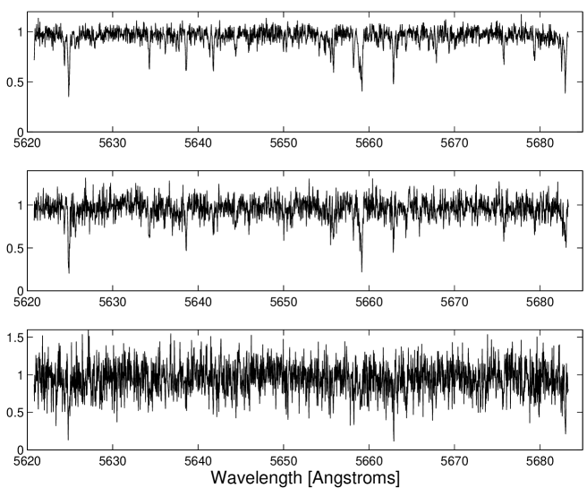
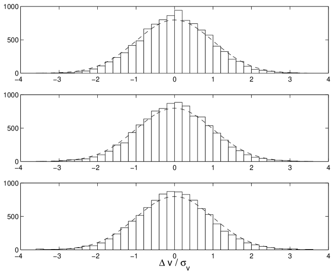
The noise added to the spectra was a simple Gaussian white noise, with standard deviations of $0.05$, $0.1$ or $0.2$. Sample noisy spectra are shown in Fig. 2. These spectra were cross-correlated against the known template, resulting in the cross-correlation functions presented in Fig. 3. The exact peak locations and the relevant derivatives were estimated by interpolating with a parabola around the peak. Each simulation was repeated $10\,000$ times. Figure 4 shows the distribution of the ratio between the actual offset of the cross-correlation peak ($\Delta v$) and the error estimate ($\sigma_{v}$). The figure shows that this ratio is distributed as a zero-mean unit-variance Gaussian for all the noise-levels tested, as we would expect for a valid error estimate. The apparent Gaussian nature of the distribution, and especially its unimodality, show the regularity of the measurement error and its estimate. In later sections we will use the same procedure to test the error estimate of the proposed combination scheme and expect to obtain similar distributions.

Figure 1: A single order from the observed multi-order spectrum of HD 38858. This order is the one used as a template for the error analysis simulation.

Figure 2: Three simulated spectra, using the template shown in Fig. 1. The noise levels used for the simulation are $0.05$ (top), $0.1$ (middle) and $0.2$ (bottom).

Figure 3: The cross-correlation functions between the spectra shown in Fig. 2 and the template (Fig. 1).

Figure 4: Histograms of the ratio between the offset of the cross-correlation function ($\Delta v$) and the estimated error ($\sigma_{v}$). The three panels correspond to the three noise levels used in Fig. 2 and 3. The dashed lines represent a zero-mean unit-variance Gaussian distribution.

3 Combining cross-correlation functions

3.1 The combination scheme

Suppose we now have $M$ separate spectra, each one corresponding to a separate template, and all are assumed to have the same Doppler shift. These separate spectra can either be separate exposures of the same object, or separate orders of the same exposure. The following analysis assumes they all possess the same number of bins – $N$, although this assumption can be very easily relaxed. We do not assume the same $S/N$ ratios for the various spectra nor the same scaling constants.

The most simple scheme to combine cross-correlation functions into one single function is the straightforward, non-weighted average ($\mathrm{SA}$):

$$\mathrm{SA}(s)=\frac{1}{M}\sum_{i=1}^{M}C_{i}(s)\ ,$$

where $M$ is the number of cross-correlation functions to be combined, while $C_{i}(s)$ is the $i$-th cross-correlation, calculated between the $i$-th spectrum and the $i$-th template.

Another simple combination scheme is based on the so-called “determination coefficient”, i.e., the squared correlation coefficient – $C^{2}(s)$ in our case. This quantity is commonly used in regression analysis to describe the degree to which the variability in one variable is explained by the other (e.g., Hays, 1988), and is supposed to be additive. Therefore, we may try to combine these determination coefficients ($\mathrm{DC}$) to get:

$$\mathrm{DC}^{2}(s)=\frac{1}{M}\sum_{i}C_{i}^{2}(s)\ .$$

This value can be interpreted as a weighted sum of the correlations. Each term is weighted by itself, since its value - the correlation - is also a measure of its reliability.

The likelihood approach can provide another scheme to combine cross-correlations. First, let us see what is the overall likelihood of the observations:

$$L=\prod_{i}\left(\frac{1}{\sqrt{2\pi\sigma_{i}^{2}}}\right)^{N}\exp{\left\{-\frac{1}{2\sigma_{i}^{2}}\sum_{n}\left[f_{i}(n)-a_{i}g_{i}(n-s)\right]^{2}\right\}}$$

Converting, as usual to the logarithm, we get:

$$\log L=-\sum_{i}\left\{N\log\sigma_{i}-\frac{1}{2\sigma_{i}^{2}}\sum_{n}\left[f(n)-a_{i}g_{i}(n-s)\right]^{2}\right\}+\mathit{const.}$$

Substituting the optimal values of $\sigma_{i}$ and $a_{i}$ leads eventually to:

$$\log L=-\frac{N}{2}\sum_{i}\log\left[1-C_{i}^{2}(s)\right]+\mathit{const.}$$

which is very similar to eq. 1. Therefore we can equate these two expressions to get an “effective” correlation value – $\mathrm{ML}$:

$$NM\log\left[1-\mathrm{ML}^{2}(s)\right]=\sum_{i}N\log\left[1-C_{i}^{2}(s)\right]$$

or:

$$\mathrm{ML}^{2}(s)=1-\left\{\prod_{i}\left[1-C_{i}^{2}(s)\right]\right\}^{1/M}$$

As it turns out, for sufficiently small $C_{i}(s)$ the above expression reduces to the expression of the “determination coefficient” mean – $\mathrm{DC}(s)$. On the other extreme, if one $C_{i}(s)$ approaches unity (meaning it has a very high $S/N$), $\mathrm{DC}(s)$ will approach unity. This can be understood intuitively, since the other cross-correlations probably represent much poorer $S/N$ and therefore can be neglected.

In order to obtain an error estimate for the shift, the Hessian of the likelihood has to be calculated and inverted. This time, the Hessian is not diagonal, but a laborious calculation yields the following expression for the error:

$$\sigma_{s}^{2}=-\bigl{[}MN\frac{\mathrm{ML}^{\prime\prime}(\hat{s})}{\mathrm{ML}(\hat{s})}\frac{\mathrm{ML}^{2}(\hat{s})}{1-\mathrm{ML}^{2}(\hat{s})}\bigr{]}^{-1}\ ,$$

which is remarkably similar to the expression for the error in the single spectrum case, except for using the total number of bins – $MN$ instead of $N$!

3.2 Simulations

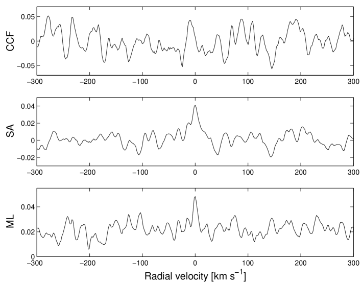
In order to demonstrate the effect of combining cross-correlations, $10$ spectral orders were used, taken from the same spectrum used in 2.4, covering the spectral range from $5\,189$ to $5\,683$ Å. As a first test, noise was added to these $10$ orders, with a very high standard deviation of $3.5$. Figure 5 presents the results of this test. The top panel shows a cross-correlation function corresponding to one of those orders. No prominent peak is present in the cross-correlation. The middle panel shows a simple average of the ten cross-correlation functions ($\mathrm{SA}$). The correct peak is evidently present. It is similarly present in the maximum-likelihood combined correlation – $\mathrm{ML}$, as the bottom panel shows. Since the cross-correlation values are very small, $\mathrm{DC}$ and $\mathrm{ML}$ are virtually identical. This simulation demonstrates the power of combining cross-correlation functions in general. In this case no velocity could have been measured for any individual order, but the cumulative effect of the $10$ orders produced a detectable peak.

Figure 5: Top: Cross-correlation function corresponding to a single order, with a noise level of $3.5$. Middle: A simple average of the cross-correlations of $10$ orders, all with a noise level of $3.5$. Bottom: maximum-likelihood combination of the same $10$ cross-correlations.

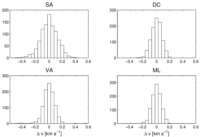
The next test shows the optimality of the maximum-likelihood scheme ($\mathrm{ML}$) compared to the two averages $\mathrm{SA}$ and $\mathrm{DC}$. This is evident mainly in cases where the $S/N$ ratio is strongly varying among the analysed spectra. To show that, noise was added to the $10$ orders with standard deviations of $0.1i$, where $i$ is the order number. Figure 6 shows the distribution of the peak offset for each of the combination schemes, after repeating the simulation for $1000$ times. In addition, the Figure also includes a histogram of the velocities derived by a weighted average of the velocities obtained from each order separately ($\mathrm{VA}$). The weighting was based on the individual error estimates. Obviously, $\mathrm{VA}$ can be calculated only if the correct peaks can be identified in the cross-correlation functions of all orders. The histogram corresponding to $\mathrm{ML}$ is evidently less dispersed than all others. Numerically, the four standard deviations corresponding to $\mathrm{SA}$, $\mathrm{DC}$, $\mathrm{VA}$ and $\mathrm{ML}$ were $0.128$, $0.078$, $0.099$ and $0.068$ $\mathrm{km\,s}^{-1}$.

Figure 6: The distribution of the peak location in each of the four combination schemes. See text for the details of the simulations. All four histograms are drawn on the same horizontal scale for the sake of comparison.

An additional criterion to distinguish among combination schemes is their ability to accentuate the correct peak relative to the spurious peaks. This ability is important for detection of faint objects, with low $S/N$. To test this ability, the typical height of the spurious peaks was estimated by the standard deviation of the function in a region that is safely distant from the correct peak. Specifically, this standard deviation was estimated on two segments of $500$ bins, on both sides of the correct peak, at a distance of at least $100$ bins from it. The mean ratios of the peak height to this standard deviation were $36$, $58$ and $65$ for $\mathrm{SA}$, $\mathrm{DC}$ and $\mathrm{ML}$, correspondingly. Once again, we see that $\mathrm{ML}$ provides the most prominent correct peak.

The above tests were repeated in numerous other conditions, in all of them $\mathrm{ML}$ was found to be the optimal scheme to combine cross-correlations.

After establishing the optimality of the maximum-likelihood combination scheme, its error estimate had to be validated, in a similar fashion to the validation done for the single spectrum case. Figure 7 shows the $\Delta v/\sigma_{v}$ calculated for the $\mathrm{ML}$ functions in the $1000$ simulations of $10$ orders. Once again, we see a very good agreement with a zero-mean unit-variance Gaussian.

Figure 7: Histogram of the ratio between the offset of the maximum-likelihood combined correlations ($\Delta v$) and the estimated error ($\sigma_{v}$). The dashed line represent a zero-mean unit-variance Gaussian distribution.

4 Concluding remarks

This paper presents a novel approach for combining cross-correlation functions. This approach is based on the relation of cross-correlation to maximum-likelihood estimation. Unlike previously suggested approaches, this approach is not based on a linear combination of the individual functions. Previous works looked for the optimal linear combination, without considering other options (e.g., Connes, 1985). In cases where the scaling constants and the signal-to-noise ratios are known, maximum-likelihood analysis will indeed lead to a linear combination. However, exact estimate of the signal-to-noise is difficult in real cases. The suggested combination does not use any such external estimate.

Although the white gaussian noise model is assumed in most analyses of the cross-correlation, it is obvious that reality is much more complex. Thus, the noise level may depend on the intensity, like in Poissonian noise, or vary across the spectrum because of illumination effects. Additional complexities mainly include long-term trends and spectral mismatch of the template to the analysed spectrum. Attempts to optimize radial-velocity measurement to deal with these problems can be based also on maximum-likelihood theory.

The suggested approach was already applied successfully to the case of HD 41004, where $30$ CORALIE orders were combined in order to detect a very faint companion of a K star (Zucker et al., 2003). The combined functions were not the conventional cross-correlation functions, but two-dimensional correlation (TODCOR) functions (Zucker & Mazeh, 1994). The successful detection of the faint companion allowed a more detailed solution of the system and confirmed earlier hypotheses of Santos et al. (2002). This case demonstrates the power of the technique to enhance the capabilities of traditional cross-correlation and improve its ability to detect and measure very faint objects, with very low $S/N$.

References

- Bouchy et al. (2001) Bouchy F., Pepe F., Queloz D., 2001, A&A, 374, 733
- Chelli (2000) Chelli A., 2000, A&A, 358, L59
- Connes (1985) Connes P., 1985, AP&SS, 110, 211
- Hays (1988) Hays W. L., 1988, Statistics, 4 edn. New York: CBS College
- Kendall & Stuart (1967) Kendall M. G., Stuart A., 1967, The Advanced Theory of Statistics. Vol. 2, London: Griffin
- Mayor & Queloz (1995) Mayor M., Queloz D., 1995, Nature, 378, 355
- Murdoch & Hearnshaw (1991) Murdoch K., Hearnshaw J. B., 1991, Ap&SS, 186, 137
- Proakis (1995) Proakis J. G., 1995, Digital Communications, 3 edn. New York: McGraw-Hill
- Santos et al. (2000) Santos N. C., Israelian G., Mayor M., 2000, A&A, 363, 228
- Santos et al. (2001) Santos N. C., Israelian G., Mayor M., 2001, A&A, 373, 1019
- Santos et al. (2002) Santos N. C., Mayor M., Naef D., Pepe F., Queloz D., Udry S., Burnet M., Clausen J. V., Helt B. E., Olsen E. H., Pritchard J. D., 2002, A&A, 392, 215
- Simkin (1974) Simkin S. M., 1974, A&A, 31, 129
- Tonry & Davis (1979) Tonry J., Davis M., 1979, AJ, 84, 1511
- Verschueren & David (1999) Verschueren W., David M., 1999, A&AS, 136, 591
- Zucker & Mazeh (1994) Zucker S., Mazeh T., 1994, ApJ, 420, 806
- Zucker et al. (2003) Zucker S., Mazeh T., Santos N. C., Udry S., Mayor M., 2003, A&A, accepted (astro-ph/0303055)