Long-term Evolution of Stellar Self-Gravitating System away from the Thermal Equilibrium : connection with non-extensive statistics

Abstract

With particular attention to the recently postulated introduction of a non-extensive generalization of Boltzmann-Gibbs statistics, we study the long-term stellar dynamical evolution of self-gravitating systems on timescales much longer than the two-body relaxation time. In a self-gravitating $N$-body system confined in an adiabatic wall, we show that the quasi-equilibrium sequence arising from the Tsallis entropy, so-called stellar polytropes, plays an important role in characterizing the transient states away from the Boltzmann-Gibbs equilibrium state.

Introduction.— The long-term evolution of self-gravitating many-body system is an old problem with a rich history in astrophysics. The problem, in nature, involves the long-range nature of attractive gravity and is fundamentally connected with statistical mechanics and thermodynamics. Historically, the important consequence from the thermodynamical arguments has arisen in 1960s, known as the gravothermal catastrophe, i.e., thermodynamic instability due to the negative specific heatBinney & Tremaine (1987). Originally, the gravothermal catastrophe has been investigated in a very idealized situation, i.e., a stellar system confined in a spherical cavityAntonov (1962). Owing to the maximum entropy principle, the existence of an unstable thermal state has been found from the standard analysis of statistical mechanics with a particular attention to the Boltzmann-Gibbs(BG) entropy:

$$S_{\rm\scriptscriptstyle BG}=-\int d^{3}\mbox{\boldmath$x$}d^{3}\mbox{\boldmath$v$}\,f(\mbox{\boldmath$x$},\mbox{\boldmath$v$})\ln f(\mbox{\boldmath$x$},\mbox{\boldmath$v$}),$$ (1)

where $f(\mbox{\boldmath$x$},\mbox{\boldmath$v$})$ denotes the one-particle distribution function defined in phase-space $(\mbox{\boldmath$x$},\mbox{\boldmath$v$})$.

Since 1960s, the standard approach using the BG entropy has dramatically improved our view of the late-time phase of the globular cluster as a real astronomical systemMeylan & Heggie (1997), however, from a thermodynamic point of view, peculiarities of the thermal property in self-gravitating systems such as negative specific heat, as well as the non-equilibrium properties away from the BG state have not yet been understood completely.

In this Letter, aiming at a better understanding of the (non-equilibrium) thermodynamic properties of stellar self-gravitating systems, we present a set of long-term $N$-body simulations, the timescale of which is much longer than the relaxation time. With a particular emphasis to the recent application of the non-extensive generalization of BG statistics, we focus on the stellar dynamical evolution in an isolated star cluster before self-similar core-collapseCohn (1980). We show that the quasi-equilibrium sequence arising from the Tsallis entropyTsallis (1988) plays an important role in characterizing the non-equilibrium evolution of a self-gravitating system.

$N$-body simulations.— The $N$-body experiment considered here is the same situation as investigated in classic papers (Antonov (1962), see also Ref.Endo, Fukushige & Makino (1997)). That is, we confine the $N$ particles interacted via Newton gravity in a spherical adiabatic wall, which reverses the radial components of the velocity if the particle reaches the wall. Without loss of generality, we set the units as $G=M=r_{e}=1$, where $G$ is gravitational constant, $M$ and $r_{e}$ is the total mass of the system and the radius of the adiabatic wall, respectively. Note that the typical timescales appearing in this system are the free-fall time, $T_{\rm ff}=(G\rho)^{-1/2}$, and the global relaxation time driven by the two-body encounter, $T_{\rm relax}=(0.1N/\ln N)T_{\rm ff}$ Binney & Tremaine (1987), which are basically scaled as $T_{\rm ff}\sim 1$ and $T_{\rm relax}\sim 0.1N/\ln N$ in our units. To perform an expensive N-body calculation, we used a special-purpose hardware, GRAPE-6, which is especially designed to accelerate the gravitational force calculations for collisional $N$-body systemsMakino (2002). With this implementation, the $4$th-order Hermite integrator with individual time stepMakino & Aarseth (1992) can work efficiently, which is suited for probing the relaxation process in denser core regions with an appropriate accuracy. We adopt the Plummer softened potential, $\phi=1/\sqrt{r^{2}+\epsilon^{2}}$ with a softening length $\epsilon$ of $1/512$ and $1/2048$.

Figure 1: Equilibrium sequences of stellar polytrope and isothermal distribution ($n=\infty$) in the energy-density contrast relation, $\lambda\equiv-r_{e}E/(GM^{2})$ v.s. $D\equiv\rho_{c}/\rho_{e}$. The thick arrows denote the evolutionary tracks in each simulation run.

Table 1: Initial distributions and their evolutionary states

run $\#$	initial distribution	parameters	$\#$ of particles	transient state	final state
A	stellar polytrope($n=3$)	$D=10,000$	2,048	stellar polytrope	collapse
B1	stellar polytrope($n=6$)	$D=110$	2,048	stellar polytrope	collapse
B2	stellar polytrope($n=6$)	$D=10,000$	2,048	stellar polytrope	collapse
C1	Hernquist model	$a/r_{e}=0.5$	8,192	stellar polytrope	collapse
C2	Hernquist model	$a/r_{e}=1.0$	8,192	none	isothermal

In the present numerical simulation, the choice of the initial condition is an important step. Here, we set the initial distribution to the stationary state of Poisson-Vlassov equation, i.e., dynamical equilibrium for a spherical system with isotropic velocity distribution. According to the Jeans theoremBinney & Tremaine (1987), the one-particle distribution function $f(\mbox{\boldmath$x$},\mbox{\boldmath$v$})$ can be expressed as a function of specific energy, $\varepsilon=v^{2}/2+\Phi(r)$ with $r$ and $\Phi$ being the radius and the gravitational potential. Then keeping the energy and the mass constant, the thermal equilibrium of ordinary extensive statistics derived from the maximum entropy principle of the BG entropy (1) reduces to the exponential distribution, so-called isothermal distribution given by $f(\varepsilon)\propto e^{-\beta\varepsilon}$, which effectively satisfies the equation of state, $P(r)\propto\rho(r)$, where $P(r)$ is pressure and $\rho(r)$ is mass densityBinney & Tremaine (1987); Antonov (1962).

On the other hand, as another possibility, one considers the extremum state of Tsallis’ non-extensive entropy Tsallis (1988):

$$S_{q}=-\int d^{3}\mbox{\boldmath$x$}d^{3}\mbox{\boldmath$v$}\,[\{f(\mbox{\boldmath$x$},\mbox{\boldmath$v$})\}^{q}-f(\mbox{\boldmath$x$},\mbox{\boldmath$v$})]/(1-q),$$ (2)

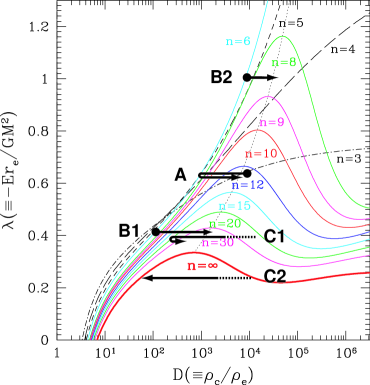
which might be of particular importance in describing the quasi-equilibrium state away from the BG stateTsallis (1999). In this case, the maximum entropy principle leads to the power-law distribution, $f(\varepsilon)\propto(\Phi_{0}-\varepsilon)^{1/(q-1)}$ Plastino & Plastino (1993); Taruya & Sakagami (2002a, b, c), referred to as the stellar polytropeBinney & Tremaine (1987). It satisfies the polytropic equation of state, $P(r)\propto\rho(r)^{1+1/n}$, and the polytrope index $n$ is related to the $q$-parameter as $n=1/(q-1)+3/2$notice_1 . Provided the polytrope index $n$, the equilibrium structure can be determined by solving the Láne-Emden equation Chandrasekhar (1939) and using this solution, the relationship between the dimensionless energy $\lambda\equiv-r_{e}E/(GM^{2})$ and the density contrast $D\equiv\rho_{c}/\rho_{e}$, the core density divided by the edge density, can be drawn (see Fig.1, notice_2 ). Note that the limit $n\to\infty$ (or $q\to 1$) corresponds to the isothermal distribution derived from the BG entropy (1).

Figure 2: Results from simulation run A. (a) Snapshots of density profile $\rho(r)$. (b) Snapshots of one-particle distribution function $f(\varepsilon)$. (c) The time evolution of the polytrope index for run A with and without the boundary of adiabatic wall.

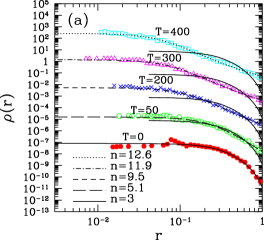
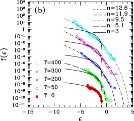
Table 1 summarizes the list of the five simulation runs. A more systematic study of the systems with several initial conditions is now in progress and the details of the results will be reported elsewhere. In Table 1, in addition to the stellar polytropic initial state, we also consider the Hernquist modelHernquist (1990), which was originally introduced to account for the empirical law of observed elliptical galaxiesBinney & Tremaine (1987).

Results.— It has been recently discussed in Taruya & Sakagami (2002a, b, c) that the thermodynamic structure of the stellar polytropic distribution can be consistently characterized by the non-extensive framework of the thermostatistics. According to their results, the stellar polytrope confined in an adiabatic wall is shown to be thermodynamically stable when the polytrope index $n<5$. In other words, if $n>5$, a stable equilibrium state ceases to exist for a sufficiently large density contrast $D>D_{\rm crit}$, where the critical value $D_{\rm crit}$ given by a function of $n$ is determined from the second variation of entropy around the extremum state of Tsallis entropy, $\delta^{2}S_{q}=0$Taruya & Sakagami (2002a, c). The dotted line in Fig.1 represents the critical value $D_{\rm crit}$ for each polytrope index, which indicates that the stellar polytrope at low density contrast $D<D_{\rm crit}$ is expected to remain stable. Apart from the BG state, one might expect that the stellar polytrope acts as a thermal equilibrium.

Figure 3: Evolution of one-particle distribution function in other models. (a) Run B1. (b) Run C1. (c) Run A removing the adiabatic wall.

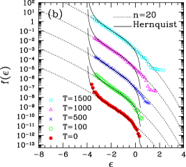
Of course, this naive expectation is not correct at all. Indeed, the numerical simulations reveal that the stellar polytropic distribution gradually changes with time, on the timescale of two-body relaxation. Further, it seems that the gravothermal instability appears at relatively smaller values of $D$ than the predicted one, $D_{\rm crit}$, which might be partially ascribed to the non-stationarity of the background stellar polytrope. Physically, the core-collapse phenomenon due to the gravothermal catastrophe follows from the decoupling of the relaxation timescales between the central and the outer parts, whose behavior sensitively depends on the physical property of heat transportMakino & Hut (1991). In a rigorous sense, the thermodynamic prediction might lose the physical relevance, however, focusing on the evolutionary sequence, we found that the transient state starting from the initial stellar polytrope can be remarkably characterized by a sequence of stellar polytropes (run A, B1 and B2). This is even true in the case starting from the Hernquist model (run C1).

Let us show the representative results taken from run A (Fig.2). Fig.2(a) plots the snapshots of the density profile $\rho(r)$, while Fig.2(b) represents the distribution function $f(\varepsilon)$ as a function of the specific energy $\varepsilon$. Note that just for illustrative purpose, each output result is artificially shifting to the two-digits below. Only the final output with $T=400$ represents the correct scales. In each figure, solid lines mean the initial stellar polytrope with $n=3$ and the other lines indicate the fitting results to the stellar polytrope by varying the polytrope index $n$notice_3 . Note that the number of fitting parameters just reduces to one, i.e., the polytrope index, since the total energy is well-conserved in the present situation. Fig.2 shows that while the system gradually deviates from the initial polytropic state, the transient state still follows a sequence of stellar polytropes. The fitting results are remarkably good until the time exceeds $T\simeq 400$, corresponding to $15T_{\rm relax}$. Afterwards, the system enters the gravothermally unstable regime and finally undergoes the core-collapse.

Now, focus on the evolutionary track in each simulation run summarized in the energy-density contrast plane (Fig.1), where the filled circle represents the initial stellar polytrope. Interestingly, the density contrast of the transient state in run A initially decreases, but it eventually turns to increase. The turning-point roughly corresponds to the stellar polytrope with index $n\sim 5-6$. Note, however, that the time evolution of polytrope index itself is a monotonically increasing function of time as shown in Fig.2(c), apart from the tiny fluctuations. This is indeed true for the other cases, indicating the Boltzmann $H$-theorem that any of the self-gravitating systems tends to approach the BG state. A typical example is the run C2, which finally reaches the stable BG state. However, as already shown in run A, all the systems cannot reach the BG state. Fig.1 indicates that no BG state is possible for a fixed value $\lambda>0.335$Antonov (1962), which can be derived from the peak value of the trajectory. Further, stable stellar polytropes cease to exist at high density contrast $D>D_{\rm crit}$. In fact, our simulations starting from the stellar polytropes finally underwent core-collapse (runs A, B1 and B2). Though it might not be rigorously correct, the predicted value $D_{\rm crit}$ provides a crude approximation to the boundary between the stability and the instability.

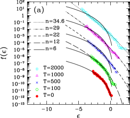
Fig.3 plots the snapshots of the distribution function taken from the other runs. The initial density contrast in run B1 (Fig.3(a)) is relatively low ($D=110$) and thereby the system slowly evolves following a sequence of stellar polytropes. After $T=2000\sim 74T_{\rm relax}$, the system begins to deviate from the stable equilibrium sequence, leading to the core-collapse. Another noticeable case is the run C1 (Fig.3(b)). The Hernquist model as initial distribution of run C has cuspy density profile, $\rho(r)\propto 1/r/(r+a)^{3}$, which behaves as $\rho\propto r^{-1}$ at the inner part Hernquist (1990). The resultant distribution function $f(\varepsilon)$ shows a singular behavior at the negative energy region, which cannot be described by the power-law distribution. Soon after a while, however, the gravothermal expansionEndo, Fukushige & Makino (1997) takes place and the flatter core is eventually formed. Then the system settles into a sequence of stellar polytropes and can be approximately described by the stellar polytrope with index $n=20$ for a long time. Thus, as long as the stellar system confined in an adiabatic wall is concerned, the stellar polytrope can be regarded as a quasi-attractor and a quasi-equilibrium state.

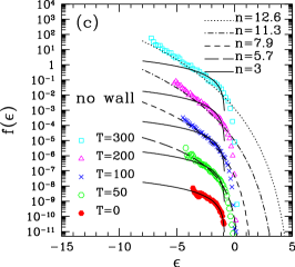
Of course, these remarkable features could be an outcome in a very idealized situation and one suspects that quasi-equilibrium state of stellar polytrope cannot hold if we remove the boundary of the adiabatic wall. As a demonstration, Fig.3(c) plots the results removing the boundary, in which the initial state is the same distribution as in run A. As is expected, the high-energy particles freely escape outwards from the central region and the resultant distribution function $f(\varepsilon)$ sharply falls off at the energy region $\varepsilon\sim 0$, indicating that the density contrast $D$ becomes effectively large. Thus, compared to the system confined in the wall, the removal of the boundary makes the stellar system unstable and the core-collapse takes place earlier. Nevertheless, focusing on the inner part of the denser region, the evolution of the core is not significantly affected by the escape particles at the outer part and can be fitted by a sequence of stellar polytropes (see also the dashed line in Fig.2(c)). The successful fit to the density profile $\rho(r)$ almost remains the same. Hence, the stellar polytrope characterized by the Tsallis entropy can be even realized in a realistic situation removing the boundary of the adiabatic wall.

Summary & Discussions.— We have performed a set of numerical simulation of long-term stellar dynamical evolution away from the BG state and found that the transient state of the system confined in an adiabatic wall can be remarkably fitted by a sequence of stellar polytropes. This is even true in the case removing the outer boundary. Therefore, the stellar polytropic distribution can be a quasi-attractor and a quasi-equilibrium state of a self-gravitating system.

Alternative characterization of the transients away from the BG state might be possible besides the $q$-exponential distribution of stellar polytropes. For an empirical characterization of observed structure, the one-parameter family of truncated exponential distributions, so-called King model has been used in the literatureBinney & Tremaine (1987); Meylan & Heggie (1997); King (1966). Also, the sequence of King model has been found to characterize the evolutionary sequence of density profile for isolated stellar systems without boundaryCohn (1980). We have also tried to fit the simulation data to the King model. Similarly to the stellar polytrope, the King model accurately describes the simulated density profile $\rho(r)$ confined in an adiabatic wall, however, it fails to match the simulated distribution function $f(\varepsilon)$, especially at the cutoff energy scales. Therefore, from the quantitative description of the entire phase-space structure, the power-law distribution of the stellar polytropes can be a better characterization of the quasi-equilibrium state and this could yield an interesting explanation of the origin of the empirical King model.

We are grateful to T. Fukushige for providing us the GRAPE-6 code and for his constant supports and helpful comments. We also thank to J. Makino for fruitful discussion especially on the applicability of equilibrium sequences of stellar polytrope. Numerical computations were carried out at ADAC (the Astronomical Data Analysis Center) of the National Astronomical Observatory of Japan. This research was supported in part by the grant-in-aid from Japan Society of Promotion of Science (No.1470157).

References

- Binney & Tremaine (1987) J. Binney and S. Tremaine, Galactic Dynamics, (Princeton Univ. Press, Princeton, 1987); L. Spitzer, Dynamical Evolution of Globular Clusters, (Princeton Univ. Press, Princeton, 1987).
- Antonov (1962) V.A. Antonov, Vest. Leningrad Gros. Univ. 7, 135 (1962); D. Lynden-Bell and R. Wood, Mon. Rot. R. Astron. Soc. 138, 495 (1968).
- Meylan & Heggie (1997) G. Meylan and D.C. Heggie, Astron. Astrophys. Rev. 8, 1 (1997).
- Cohn (1980) H. Cohn, Astrophys. J. 242, 765 (1980).
- Tsallis (1988) C. Tsallis, J. Stat. Phys. 52, 479 (1988).
- Endo, Fukushige & Makino (1997) H. Endoh, T. Fukushige and J. Makino, Publ. Astron. Soc. Japan 49, 345 (1997).
- Makino (2002) J. Makino, in J. Makino and P. Hut (Eds.), Proc. IAU Symp. 208, Astrophysical Supercomputing using Particle Simulations, in press.
- Makino & Aarseth (1992) J. Makino and S.J. Aarseth, Publ. Astron. Soc. Japan 44, 141 (1992).
- Tsallis (1999) C. Tsallis, Braz. J. Phys. 29 1; S. Abe and Y. Okamoto (Eds.), Nonextensive Statistical Mechanics and Its Applications (Springer, Berlin, 2001).
- Plastino & Plastino (1993) A.R. Plastino and A. Plastino, Phys. Lett. A 174, 384 (1993).
- Taruya & Sakagami (2002a) A. Taruya and M. Sakagami, Physica A 307, 185 (2002).
- Taruya & Sakagami (2002b) A. Taruya and M. Sakagami, Physica A 318, 387 (2003).
- Taruya & Sakagami (2002c) A. Taruya and M. Sakagami, Physica A (2003), in press (cond-mat/0211305).
- (14) The relation between the polytrope index and the -parameter may change, depending on the choice of the statistical average: standard linear meansPlastino & Plastino (1993); Taruya & Sakagami (2002a) or normalized -valuesTaruya & Sakagami (2002c). Here, we simply adopt the result using the standard linear mean.
- Chandrasekhar (1939) S. Chandrasekhar, Introduction to the Study of Stellar Structure, (Dover, New York, 1939).
- (16) The energy-density contrast relation in Fig.1 is essentially the same one as obtained from the analysis using the standard linear means (Fig.2 of Ref.Taruya & Sakagami (2002a)) and that using the normalized -values (Fig. 3 of Ref.Taruya & Sakagami (2002c)). This means that the thermodynamic stability in a system confined in an adiabatic wall does not depend on the choice of the statistical average (see Ref.Taruya & Sakagami (2002c) for details).
- Hernquist (1990) L. Hernquist, Astrophys. J. 356, 359 (1990).
- Makino & Hut (1991) J. Makino and P. Hut, Astrophys. J. 383, 181 (1991).
- (19) In fitting the simulation data to the stellar polytrope, we first quantify the radial density profile from each snapshot data. Selecting the points from it at regular intervals in logarithmic scale of radius , the results are then compared with the Emden solutions, fixing the energy and varying the polytrope index .
- King (1966) I.R. King, Astron. J. 71 64 (1966).