Constraining the dark energy with galaxy clusters X-ray data

Abstract

The equation of state characterizing the dark energy component is constrained by combining Chandra observations of the X-ray luminosity of galaxy clusters with independent measurements of the baryonic matter density and the latest measurements of the Hubble parameter as given by the HST key project. By assuming a spatially flat scenario driven by a “quintessence” component with an equation of state $p_{x}=\omega\rho_{x}$ we place the following limits on the cosmological parameters $\omega$ and $\Omega_{\rm{m}}$: (i) $-1\leq\omega\leq-0.55$ and $\Omega_{\rm m}=0.32^{+0.027}_{-0.014}$ (1$\sigma$) if the equation of state of the dark energy is restricted to the interval $-1\leq\omega<0$ (usual quintessence) and (ii) $\omega=-1.29^{+0.686}_{-0.792}$ and $\Omega_{\rm{m}}=0.31^{+0.037}_{-0.034}$ ($1\sigma$) if $\omega$ violates the null energy condition and assume values $<-1$ (extended quintessence or “phantom” energy). These results are in good agreement with independent studies based on supernovae observations, large-scale structure and the anisotropies of the cosmic background radiation.

I Introduction

Recent observations of Type Ia supernovae (SNe Ia) have provided direct evidence that the universe may be accelerating perlmutter . These results, when combined with measurements of cosmic microwave background radiation (CMB) anisotropies and dynamical estimates of the quantity of matter in the Universe, suggest a spatially flat universe composed of nearly $\sim 1/3$ of matter (baryonic + dark) and $\sim 2/3$ of an exotic component endowed with large negative pressure, the so-called “quintessence”. Nowadays, it has been promptly recognized that the question related to the nature of this dark energy is one of the most challenging problems of modern astrophysics, cosmology and particle physics.

The absence of a natural guidance from particle physics theory about the nature of this dark component gave origin to an intense debate and many theoretical speculations. In particular, a cosmological constant ($\Lambda$) – the most natural candidate – is the simplest but not the unique possibility; $\Lambda$ is a time independent and spatially uniform dark component, which is described by a perfect fluid with $p_{v}=-\rho_{v}$. Some other candidates appearing in the literature are: a decaying vacuum energy density, or a time varying $\Lambda$-term ozer , a time varying relic scalar field component (SFC) which is slowly rolling down its potencial ratra , the so-called “X-matter”, an extra component simply characterized by an equation of state $p_{\rm x}=\omega\rho_{\rm x}$ (XCDM) turner ; tchiba , the Chaplygin gas whose equation of state is given by $p=-A/\rho$ where $A$ is a positive constant bert , models based on the framework of brane-induced gravity dvali , among others mcreation . For SFC and XCDM scenarios, the $\omega$ parameter may be a function of the redshift (see, for example, efs ) or still, as has been recently discussed, it may violate the null energy condition and assume values $<-1$ leq1 .

In order to improve our understanding of the actual nature of the dark energy, an important task nowadays in cosmology is to find new methods or to revive old ones that could directly or indirectly quantify the amount of dark energy present in the Universe, as well as determine its equation of state. In this concern, the possibility of constraining cosmological parameters from X-ray luminosity of galaxy clusters constitutes an important and interesting tool. This method was originally proposed by Sasaki sasa and Pen pen with basis on measurements of the mean baryonic mass fraction in clusters as a function of redshift. A recent application of a new version of this test was performed by Allen et al. allen ; allen1 (see also ett ) who analyzed the X-ray observations in some relaxed lensing clusters observed with Chandra spanning the redshift range $0.1<z<0.5$. By inferring the corresponding gas mass fraction they placed observational limits on the total matter density parameter, $\Omega_{\rm m}$, as well as on the density parameter, $\Omega_{\Lambda}$, associated to the vacuum energy density.

In the present paper, by following the methodology presented in allen1 , we discuss quantitatively how the observations of X-ray gas mass fraction of galaxy clusters constrains the cosmic equation of state describing the dark energy component. In order to detect the possibility of bias in the parameter determination due to the imposition $\omega\geq-1$ we have studied two different cases: the usual quintessence ($-1\leq\omega<0$) and the extended quintessence (also named “phantom” energy leq1 ), in which the $\omega$ parameter may assume values $<-1$. In the former case, a good agreement between theory and observations is possible if $0.3\leq\Omega_{\rm m}\leq 0.35$ ($68\%$ c.l.) and $\omega\leq-0.55$. These results are in line with recent analyzes from distant SNe Ia garn , SNe + CMB efs , gravitational lensing statistics class and the existence of old high redshift objects (OHRO’s) alcaniz1 . For extended quintessence we obtain $-2.1\leq\omega\leq-0.6$ ($68\%$ c.l.) with the matter density parameter ranging in the interval $0.27\leq\Omega_{\rm m}\leq 0.34$ ($68\%$ c.l.).

This paper is organized as follows. In Section II we present the basic field equations and the distance formulas relevant for our analysis. The corresponding constraints on the cosmological parameters $\omega$ and $\Omega_{\rm{m}}$ are investigated in Section III. We finish the paper by summarizing the main results in the conclusion Section.

II Basic equations

For a spatially flat, homogeneous, and isotropic cosmologies driven by nonrelativistic matter and a separately conserved exotic fluid with equation of state, $p_{x}=\omega\rho_{x}$, the Friedman’s equation is given by:

$$({\dot{R}\over R})^{2}=H_{o}^{2}\left[\Omega_{\rm{m}}({R_{o}\over R})^{3}+(1-\Omega_{\rm{m}})({R_{o}\over R})^{3(1+\omega)}\right],$$ (1)

where an overdot denotes derivative with respect to time and $H_{o}=100h{\rm{Km.s^{-1}.Mpc^{-1}}}$ is the present value of the Hubble parameter.

In order to derive the constraints from X-ray gas mass fraction in the next Section we shall use the concept of angular diameter distance, $D_{A}(z)$. Such a quantity can be easily obtained in the following way: consider that photons are emitted by a source with coordinate $r=r_{1}$ at time $t_{1}$ and are received at time $t_{o}$ by an observer located at coordinate $r=0$. The emitted radiation will follow null geodesics so that the comoving distance of the source is defined by ($c=1$)

$$r_{1}=\int_{t_{1}}^{t_{o}}{dt\over R(t)}=\int_{R(t)}^{R_{o}}{dR\over\dot{R}(t)R(t)}.$$ (2)

By considering the above equations, it is straightforward to show that the comoving distance $r_{1}(z)$ can be written as

$$r_{1}(z)=\frac{1}{H_{o}R_{o}}\int_{\frac{1}{1+z}}^{1}{dx\over x\sqrt{\Omega_{\rm{m}}x^{-1}+(1-\Omega_{\rm{m}})x^{-(1+3\omega)}}},$$ (3)

where the subscript $o$ denotes present day quantities and $x={R(t)\over R_{o}}=(1+z)^{-1}$ is a convenient integration variable. The angular diameter distance to a light source at $r=r_{1}$ and $t=t_{1}$ which is observed at $r=0$ and $t=t_{o}$ is defined as the ratio of the source diameter to its angular diameter, i.e.,

$$D_{A}={\ell\over\theta}=R(t_{1})r_{1}=(1+z)^{-1}R_{o}r(z),$$ (4)

which provides, when combined with Eq. (3),

$$D_{\rm A}^{\rm{DE}}=\frac{H_{o}^{-1}}{(1+z)}\int_{\frac{1}{1+z}}^{1}{dx\over x\sqrt{\Omega_{\rm{m}}x^{-1}+(1-\Omega_{\rm{m}})x^{-(1+3\omega)}}}.$$ (5)

For the standard cold dark matter model (SCDM) we set $\omega=0$ in Eq. (3) and the angular diameter distance reduces to

$$D_{\rm A}^{\rm{SCDM}}=\frac{2H_{o}^{-1}}{(1+z)^{3/2}}\left[(1+z)^{1/2}-1\right].$$ (6)

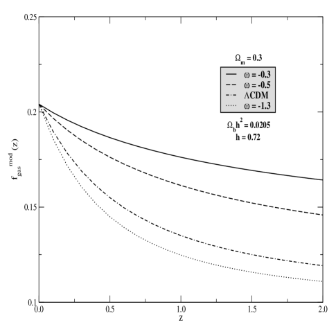
Figure 1: The model function $f_{\rm gas}^{\rm mod}$ (Eq. 8) as a function of the redshift for selected values of $\omega$ and fixed values of $\Omega_{\rm{m}}=0.3$, $\Omega_{\rm b}h^{2}=0.0205$ and $h=0.72$.

III Constraints from X-ray gas mass fraction

In our analysis we consider the Chandra data analysed in recent papers by Allen et al.allen ; allen1 and Schmidt et al.schim . The specific data set consists of six clusters distributed over a wide range of redshifts ($0.1<z<0.5$). The clusters studied are all regular, relatively relaxed systems for which independent confirmation of the matter density parameter results is available from gravitational lensing studies. As discussed in Ref. allen1 , the systematic uncertainties are $\lesssim 10\%$ (i.e. typically smaller than the statistical uncertainties). The X-ray gas mass fraction ($f_{\rm gas}$) values were determined for a canonical radius $r_{2500}$, which is defined as the radius within which the mean mass density is 2500 times the critical density of the Universe at the redshift of the cluster. Two data sets were generated from these data. One in which the SCDM model with $H_{o}=50{\rm{Km.s^{-1}.Mpc^{-1}}}$ is used as the default cosmology and the other one in which the default cosmology is the $\Lambda$CDM scenario with $H_{o}=70{\rm{Km.s^{-1}.Mpc^{-1}}}$, $\Omega_{\rm{m}}=0.3$ and $\Omega_{\Lambda}=0.7$. In what follows we constrain the basic cosmological parameters using the SCDM scenario as the default cosmology.

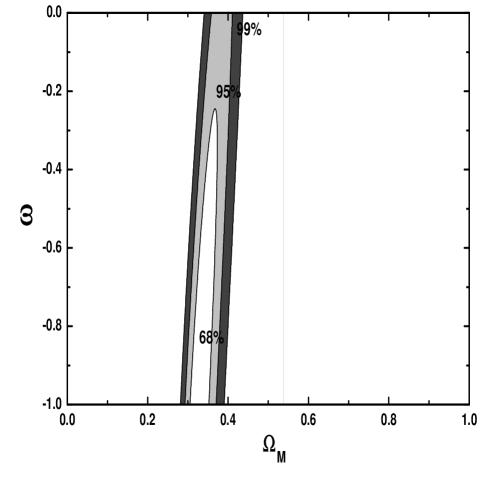
Figure 2: Confidence regions in the $\Omega_{\rm{m}}-\omega$ plane by assuming the SCDM model as the default cosmology. The regions in the graph correspond to 68%, 95% and 99% likelihood contours for flat quintessence scenarios.

By assuming that the baryonic mass fraction in galaxy clusters provides a fair sample of the distribution of baryons at large scale, the matter content of the universe can be expressed as white ; hogan :

$$\Omega_{\rm m}=\frac{\Omega_{\rm b}}{f_{\rm gas}(1+0.19h^{3/2})},$$ (7)

where $\Omega_{\rm b}$ stands for the baryonic mass density parameter. Since $f_{\rm gas}\propto D_{\rm{A}}^{3/2}$ sasa , the model function is defined by

$$f_{\rm gas}^{\rm mod}(z_{\rm i})=\frac{\Omega_{\rm b}}{\left(1+0.19{h}^{3/2}\right)\Omega_{\rm m}}\left[2h\,\frac{D_{\rm A}^{\rm{SCDM}}(z_{\rm i})}{D_{\rm A}^{\rm{DE}}(z_{\rm i})}\right]^{1.5},$$ (8)

where the term $(2h)^{3/2}$ represents the change in the Hubble parameter between the default cosmology and quintessence scenarios while the ratio ${D_{\rm A}^{\rm{SCDM}}(z_{\rm i})}/{D_{\rm A}^{\rm{DE}}(z_{\rm i})}$ accounts for deviations in the geometry of the universe from the SCDM model. Figure 1 shows the behavior of $f_{\rm gas}^{\rm mod}$ as a function of the redshift for some selected values of $\omega$ having the values of $\Omega_{\rm b}$ and $h$ fixed. The value of $\Omega_{\rm m}$ is fixed at $0.3$ as suggested by dynamical estimates on scales up to about $2h^{-1}$ Mpc calb . For the sake of comparison, the current favored cosmological model, namely, a flat scenario with $70\%$ of the critical energy density dominated by a cosmological constant ($\Lambda$CDM) is also shown.

In order to determine the cosmological parameters $\Omega_{\rm{m}}$ and $\omega$ we use a $\chi^{2}$ minimization for the range of $\Omega_{\rm{m}}$ and $\omega$ spanning the interval [0,1] in steps of 0.02

$$\chi^{2} = \sum_{i=1}^{6}\frac{\left[f_{\rm gas}^{\rm mod}(z_{\rm i})-f_{\rm gas,\,i}\right]^{2}}{\sigma_{f_{\rm gas,\,i}}^{2}}$$ (9)

where $\sigma_{f_{\rm gas,\,i}}$ are the symmetric root-mean-square errors for the SCDM data. The $68.3\%$ and $95.4\%$ confidence levels are defined by the conventional two-parameters $\chi^{2}$ levels 2.30 and 6.17, respectively.

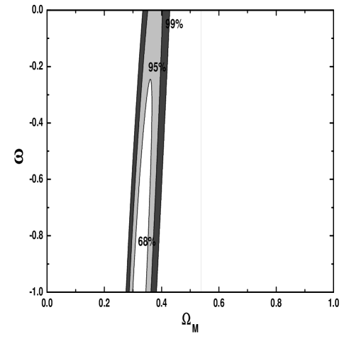
Figure 3: The same as in Fig. 2 by assuming the Gaussian priors $h=0.72\pm 0.08$ and $\Omega_{\rm b}h^{2}=0.0205\pm 0.0018$.

In Fig. 2, by fixing the values of $\Omega_{\rm b}$ (0.0205) and $h$ (0.72), we show contours of constant likelihood (95% and 68%) in the $\Omega_{\rm m}$-$\omega$ plane. Note that the allowed range for both $\Omega_{\rm m}$ and $\omega$ is reasonably large, showing the impossibility of placing restrictive limits on these quintessence scenarios from the considered X-ray gas mass fraction data. The best-fit model for these data occurs for $\Omega_{\rm m}=0.33$ and $\omega=-1.0$ with $\chi^{2}=1.98$. Such limits become slightly more restrictive if we assume some a priori knowledge of the value of the product $\Omega_{\rm b}h^{2}=0.0205\pm 0.0018$ omera and of the value of the Hubble parameter $h=0.72\pm 0.08$ freedman . To illustrate these new results, in Fig. 3 we show the confidence regions in the $\Omega_{\rm m}$-$\omega$ plane by assuming such priors. In this case, the best-fit model occurs for $\Omega_{\rm m}=0.32$, $\omega=-1$ and $\chi^{2}_{\rm min}=1.95$ with the 1-$\sigma$ limits on $\omega$ and $\Omega_{\rm m}$ given, respectively, by

$$\omega\leq-0.555,$$

and

$$\Omega_{\rm{m}}=0.320^{+0.027}_{-0.014}.$$

For the sake of completeness, we also verified that by fixing $\omega=-1$ and extending the analysis for arbitrary geometries the results of allen1 are fully recovered.

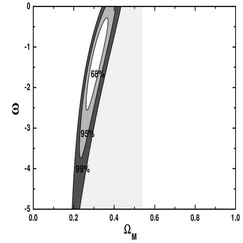
Figure 4: Constraints on the $\Omega_{\rm{m}}-\omega$ plane for extended quintessence. The regions in the graph correspond to 68%, 95% and 99% confidence limits. As in Fig. 3, Gaussian priors on the values of $\Omega_{\rm{b}}h^{2}$ and $h$ were assumed.

So far we have assumed that the dark energy equation of state is constrained to be $\omega\geq-1$. However, as has been observed recently a dark component with $\omega<-1$ appears to provide a better fit to SNe Ia observations than do $\Lambda$CDM scenarios ($\omega=-1$) leq1 . In fact, although having some unusual properties, this “phantom” behavior is predicted by several scenarios as, for example, kinetically driven models chiba1 and some versions of brane world cosmologies sahni (see also mcI and references therein). In this concern, a natural question at this point is: how does this extension of the parameter space to $\omega<-1$ modify the previous results? To answer this question in Fig. 4 we show the 68% and 95% confidence regions in the “extended” $\Omega_{\rm{m}}-\omega$ plane by assuming the same a priori knowledge of the product $\Omega_{\rm b}h^{2}$ and of the value of the Hubble parameter as done earlier. From this analysis, we find $\Omega_{\rm m}=0.312^{+0.037}_{-0.034}$, $\omega=-1.29^{+0.686}_{-0.792}$ and $\chi^{2}_{\rm min}=1.77$ both results at 1-$\sigma$ level. By assuming no a priori knowledge on $\Omega_{\rm b}h^{2}$ and $h$ we obtain $\omega=-1.28^{+0.682}_{-0.809}$ while the value of $\Omega_{\rm{m}}$ remains approximately the same. These limits should be compared with the ones obtained by Hannestad & Mörtsell hann by combining CMB + Large Scale Structure (LSS) + SNe Ia data. At 95.4% c.l. they found $-2.68<\omega<-0.78$.

Table 1: Limits to $\Omega_{\rm{m}}$ and $\omega$

Method	Reference	$\Omega_{\rm{m}}$	$\omega$
CMB + SNe Ia:…..	turner	$\simeq 0.3$	$\simeq-0.6$
	efs	$\sim$	$<-0.6$
SNe Ia………………..	garn	$\sim$	$<-0.55$
SNe Ia + GL……….	waga	$0.24$	$<-0.7$
GL……………………..	class	$\sim$	$-0.55$
SNe Ia + LSS………	perl	$\sim$	$<-0.6$
Various……………….	wang	$0.2-0.5$	$<-0.6$
OHRO’s………………	alcaniz1	0.3	$\leq-0.27$
CMB…………………..	balbi	0.3	$<-0.5$
	cora	$\sim$	$<-0.96$
$\Delta\theta$……………………..	jain	0.2-0.4	$\leq-0.5$
$\theta(z)$…………………….	jsa	0.2	$\simeq-1.0$
CMB + SNe + LSS.	bean	0.3	$<-0.85$
CMB + SNe + LSS.	hann	$\sim$	$<-0.71$
CMB + SNe + LSS.	hann	$\sim$	$>-2.68$
SNe Iaa……………….	hann	0.45	$-1.9$
SNe + X-ray Clusters a..	schu	$\simeq 0.29$	$-0.95$
X-ray Clusters…….	This Paper	$\simeq 0.32$	$\leq-0.5$
X-ray Clusters a…….	This Paper	$\simeq 0.31$	$-1.29$

At this point we compare our results with other recent determinations of $\omega$ derived from independent methods. For example, for the usual quintessence (i.e., $\omega\geq-1$), Garnavich et al. garn used the SNe Ia data from the High-$z$ Supernova Search Team to find $\omega<-0.55$ ($95\%$ c.l.) for flat models whatever the value of $\Omega_{\rm{m}}$ whereas for arbitrary geometry they obtained $\omega<-0.6$ ($95\%$ c.l.). Such results agree with the constraints obtained from a wide variety of different phenomena, using the “concordance cosmic” method wang . In this case, the combined maximum likelihood analysis suggests $\omega\leq-0.6$, which rules out an unknown component like topological defects (domain walls and string) for which $\omega=-\frac{n}{3}$, being $n$ the dimension of the defect. Recently, Lima and Alcaniz jsa investigated the angular size - redshift diagram ($\theta(z)$) in quintessence models by using the Gurvits’ published data set gurv . Their analysis sugests $-1\leq\omega\leq-0.5$ whereas Corasaniti and Copeland cora found, by using SNe Ia data and measurements of the position of the acoustic peaks in the CMB spectrum, $-1\leq\omega\leq-0.93$ at $2\sigma$. More recently, Jain et al. jain used image separation distribution function ($\Delta\theta$) of lensed quasars to obtain $-0.8\leq\omega\leq-0.4$, for the observed range of $\Omega_{m}\sim 0.2-0.4$ while Chae et al. class used gravitational lens (GL) statistics based on the final Cosmic Lens All Sky Survey (CLASS) data to find $\omega<-0.55^{+0.18}_{-0.11}$ (68% c.l.). Bean and Melchiorri bean obtained $\omega<-0.85$ from CMB + SNe Ia + LSS data, which provides no significant evidence for quintessential behaviour different from that of a cosmological constant. A similar conclusion was also obtained by Schuecker et al. schu from an analysis involving the REFLEX X-ray cluster and SNe Ia data in which the condition $\omega\geq-1$ was relaxed. A more extensive list of recent determinations of the quintessence parameter $\omega$ is presented in Table I.

IV Conclusion

The determination of cosmological parameters is a central goal of modern cosmology. We live in a special moment where the emergence of a new “standard cosmology” driven by some form of dark energy seems to be inevitable. The uncomfortable situation for some comes from the fact that the emerging model is somewhat more complicated physically speaking, while for others it is exciting because although preserving some aspects of the basic scenario a new invisible actor which has not been predicted by particle physics is coming into play.

Using the reasonable ansatz of constant gas mass fraction at large scale, we placed new limits on the $\Omega_{\rm m}$ and $\omega$ parameters for a flat dark energy model. The galaxy cluster data used corresponds to regular, relaxed systems whose $f_{\rm gas}(r)$ profiles are essentially flat around $r_{2500}$, the mass results were confirmed from gravitational lensing studies and the residual systematic uncertainties in the $f_{\rm gas}$ values are small allen1 . Naturally, the analysis presented here also reinforces the interest in searching for X-ray data both for less relaxed clusters, and perhaps more important, at higher redshifts. Hopefully, our constraints will be more stringent when further Chandra, XMM-Newton and more accurate gravitational lensing data for clusters become available near future. In this concern, we recall that X-ray data from galaxy clusters at high redshifts and the corresponding constraints for $\Omega_{m}$ will play a key hole in the coming years because their relative abundance (and consequently the value of $\Omega_{m}$ itself) may also independently be checked trough the Sunyaev-Zeldovich effectC2003 .

As we have seen, the X-ray data at present also favor eternal expansion as the fate of the Universe in accordance with SNe Ia dataperlmutter . Our estimates of $\Omega_{\rm m}$ and $\omega$ are compatible with the results obtained from many independent methods (see Table I). We emphasize that a combination of these X-ray data with different methods is very welcome not only because of the gain in precision but also because most of cosmological tests are endowed with a high degree of degeneracy and may constrain rather well only specific combinations of cosmological parameters but not each parameter individually. The basic results combining different methods will appear in a forthcoming communication next .

- (1) S. Perlmutter et al., Nature, 391, 51 (1998); S. Perlmutter et al., Astrophys. J. 517, 565 (1999); A. Riess et al., Astron. J. 116, 1009 (1998).
- (2) M. Ozer and O. Taha, Nucl. Phys. B287, 776 (1987); K. Freese, F. C. Adams, J. A. Frieman and E. Mottola, Nucl. Phys. B287, 797 (1987); J. C. Carvalho, J. A. S. Lima and I. Waga, Phys. Rev. D46 2404 (1992); F. M. Overduin and F. I. Cooperstock, Phys. Rev. D58, 043506 (1998); J. V. Cunha, J. A. S. Lima and J. S. Alcaniz, Phys. Rev. D66, 023520 (2002); J. S. Alcaniz and J. M. F. Maia, Phys. Rev. D67, 043502 (2003).
- (3) B. Ratra and P. J. E. Peebles, Phys. Rev. D37, 3406 (1988); J. A. Frieman, C. T. Hill, A. Stebbins and I. Waga, Phys. Rev. Lett. 75, 2077 (1995); R. R. Caldwell, R. Dave and P. J. Steinhardt, Phys. Rev. Lett. 80, 1582 (1998); T. D. Saini, S. Raychaudhury, V. Sahni and A. A. Starobinsky, Phys. Rev. Lett. 85, 1162 (2000); R. R. Caldwell, Braz. J. Phys. 30, 215 (2000).
- (4) M. S. Turner and M. White, Phys. Rev. D56, R4439 (1997).
- (5) T. Chiba, N. Sugiyama and T. Nakamura, Mon. Not. Roy. Astron. Soc. 289, L5 (1997); J. S. Alcaniz and J. A. S. Lima, Astrophys. J. 550, L133 (2001); J. Kujat, A. M. Linn, R. J. Scherrer and D. H. Weinberg, Astrophys. J. 572, 1 (2002); D. Jain, A. Dev, N. Panchapakesan, S. Mahajan, V. B. Bhatia, astro-ph/0105551.
- (6) A. Kamenshchik, U. Moschella and V. Pasquier, Phys. Lett. B511, 265 (2001); M. C. Bento, O Bertolami and A. A. Sen, Phys. Rev. D66, 043507 (2002); A. Dev, D. Jain and J. S. Alcaniz, Phys. Rev. D67, 023515 (2003); M. C. Bento, O. Bertolami and A. A. Sen, astro-ph/0210468; J. S. Alcaniz, D. Jain and A. Dev., Phys. Rev. D67, 043514 (2003). astro-ph/0210476; D. Carturan and F. Finelli, astro-ph/0211626; H. Sandvik, M. Tegmark, M. Zaldarriaga and I. Waga, astro-ph/0212114; U. Alam, V. Sahni, T. D. Saini and A. A. Starobinsky, astro-ph/0303009; R. Colistete Jr, J. C. Fabris, S.V.B. Gon alves and P.E. de Souza, astro-ph/0303338
- (7) G. Dvali, G. Gabadadze and M. Porrati, Phys. Lett. B485, 208 (2000); C. Deffayet, Phys. Lett. B502, 199 (2001); J. S. Alcaniz, Phys.Rev. D65, 123514 (2002). astro-ph/0202492; J. S. Alcaniz, D. Jain and A. Dev, Phys. Rev. D66, 067301 (2002); D. Jain, A. Dev and J. S. Alcaniz, Phys. Rev. D66, 083511 (2002)
- (8) J. A. S. Lima and J. S. Alcaniz, Astron. Astrophys. 348, 1 (1999); J. S. Alcaniz and J. A. S. Lima, Astron. Astrophys. 349, 729 (1999); P. Chimento, A. S. Jakubi and N. A. Zuccala, Phys. Rev. D63, 103508 (2001); W. Zimdahl, D. J. Schwarz, A. B. Balakin and Diego Pavón, Phys. Rev. D64, 063501 (2001); M. P. Freaza, R. S. de Souza and I. Waga, Phys. Rev. D66, 103502 (2002); K. Freese and M. Lewis, Phys. Lett. B540, 1 (2002); Z. Zhu and M. Fujimoto, Astrophys. J. 581, 1 (2002).
- (9) G. Efstathiou, Mon. Not. Roy. Astron. Soc. 310, 842 (1999).
- (10) R. R. Caldwell, Phys. Lett. B545, 23 (2002).
- (11) S. Sasaki, PASJ, 48, L119 (1996).
- (12) U. Pen, New Astron. 2, 309 (1997).
- (13) S. W. Allen, S. Ettori, A. C. Fabian, MNRAS, 324, 877 (2002)
- (14) S. W. Allen, R. W. Schmidt, A. C. Fabian, MNRAS, 334, L11 (2002).
- (15) S. Ettori, P. Tozzi and P. Rosati, Astron. Astrophys. 398, 879 (2003).
- (16) P. M. Garnavich et al., Astrophys. J. 509, 74 (1998).
- (17) K.-H. Chae et al., Phys. Rev. Lett. 89, 151301 (2002).
- (18) J. A. S. Lima and J. S. Alcaniz, Mon. Not. Roy. Astron. Soc. 317, 893 (2000); J. S. Alcaniz, J. A. S. Lima and J.V. Cunha, Mon. Not. Roy. Astron. Soc. (2003), in press. See also astro-ph/0301226.
- (19) R.W. Schmidt, S.W. Allen, A.C. Fabian, MNRAS, 327, 1057 (2001).
- (20) S. D. M. White, J. F. Navarro, A. E. Evrard, C. S. Frenk, Nature, 366, 429 (1993).
- (21) M. Fukugita, C. J. Hogan, P.J.E Peebles, Astrophys. J. , 503, 518 (1998).
- (22) R. G. Calberg et al., Astrophys. J. 462, 32 (1996); A. Dekel, D. Burstein and S. White S., In Critical Dialogues in Cosmology, edited by N. Turok World Scientific, Singapore (1997).
- (23) J.M. O’Meara, D. Tytler, D. Kirkman, N. Suzuki, J. X. Prochaska, D. Lubin, A. M. Wolfe, Astrophys. J. , 552, 718 (2001).
- (24) W. Freedman et al., Astrophys. J. , 553, 47 (2001).
- (25) T. Chiba, T. Okabe and M. Yamaguchi, Phys. Rev. D 62, 023511 (2000).
- (26) V. Sahni and Y. Shtanov, astro-ph/0202346.
- (27) B. McInnes, astro-ph/0210321; S. M. Carroll, M. Hoffman and M. Trodden, astro-ph/0301273
- (28) S. Hannestad and E. Mörtsell, Phys. Rev D 66, 063508 (2002)
- (29) L. Wang, R. R. caldwell, J. P. Ostriker & P. J. Steinhardt, Astrophys. J. 530, 17 (2000).
- (30) J. A. S. Lima and J. S. Alcaniz, Astrophys. J. 566, 15 (2002).
- (31) L. I. Gurvits, K. I. Kellermann and S. Frey, A&A 342, 378 (1999).
- (32) P. S. Corasaniti and E. J. Copeland, Phys. Rev. D65, 043004 (2002).
- (33) D. Jain, A. Dev, N. Panchapakesan, S. Mahajan, V. B. Bhatia, astro-ph/0105551.
- (34) R. Bean and A. Melchiorri, Phys. Rev. D65, 041302(R) (2002).
- (35) P. Schuecker, R. R. Caldwell, H. Bohringer, C. A. Collins and Luigi Guzzo, astro-ph/0211480.
- (36) I. Waga and A. P. M. R. Miceli, Phys. Rev 59, 103507.
- (37) S. Perlmutter, M. S. Turner and M. White, Phys. Rev. Lett. 83, 670 (1999).
- (38) A. Balbi, C. Baccigalupi, S. Matarrese, F. Perrota and N. Vitorio, Astrophys. J. 547, L89 (2001).
- (39) J. E. Carlstrom, G. P. Holder and E. D. Reese, Ann. Rev. Astronom. Astrophys., (2003). In press.
- (40) J. V. Cunha, J. S. Alcaniz and J. A. S. Lima, in preparation.