Explosive reconnection in magnetars

Abstract

X-ray activity of Anomalous X-ray Pulsars and Soft Gamma-Ray Repeaters may result from the heating of their magnetic corona by direct currents dissipated by magnetic reconnection. We investigate the possibility that X-ray flares and bursts observed from AXPs and SGRs result from magnetospheric reconnection events initiated by development of tearing mode in magnetically-dominated relativistic plasma. We formulate equations of resistive force-free electrodynamics, discuss its relation to ideal electrodynamics, and give examples of both ideal and resistive equilibria. Resistive force-free current layers are unstable toward the development of small-scale current sheets where resistive effects become important. Thin current sheets are found to be unstable due to the development of resistive force-free tearing mode. The growth rate of tearing mode is intermediate between the short Alfvén time scale $\tau_{A}$ and a long resistive time scale $\tau_{R}$: $\Gamma\sim 1/(\tau_{R}\tau_{A})^{1/2}$, similar to the case of non-relativistic non-force-free plasma. We propose that growth of tearing mode is related to the typical rise time of flares, $\sim 10$ msec. Finally, we discuss how reconnection may explain other magnetar phenomena and ways to test the model.

1 Introduction

Two closely related classes of young neutron stars – Anomalous X-ray Pulsars (AXPs) and the Soft Gamma-ray Repeaters (SGRs) – both show X-ray flares and, once localized, quiescent X-ray emission (Kouveliotou et al. 1998, Gavriil et al. 2002; for recent reviews see Mereghetti 2000, Thompson 2001). The energy powering the X-ray luminosity in these sources is supplied by the dissipation of super-strong magnetic fields, $B>10^{15}$G (Thompson & Duncan 1996). Hence the two classes are commonly referred to as magnetars. Magnetic fields are formed through a dynamo action during supernova collapse (Duncan & Thompson 1992, Thompson & Murray 2001).

A number of evidence suggest that processes that lead to the production of X-ray flares (and possibly of the persistent emission) on magnetars is similar to those operating in Solar corona (see also Section 6; for alternative model addressing persistent emission see Heyl & Hernquist 1998). The bursting activity of SGRs is strongly intermittent (good statistics for the AXPs’ bursting properties does not exists yet). The studies of statistics of SGR bursts from SGR 1900+14 (Gögüs et al. 1999) have found a power law dependence of the number of flares on their energy, $dN/dE\sim E^{\alpha}$, with $\alpha=1.66$; this is similar to solar flares, where $\alpha=1.5-1.7$ (Aschwanden et al. 2001). The distribution of time intervals between successive bursts from SGR 1900+14 is consistent with a log-normal distribution, also similar to the Sun (Gögüs et al. 1999). In addition, Woods et al. (2001) have argued that the magnetic field of the neutron star in SGR 1900+14 was significantly altered (perhaps globally) during the giant flare. Given these similarities, a suggestion that magnetar bursts originate in the current-carrying magnetospheres is only natural.

Thompson, Lyutikov and Kulkarni (2002) have investigated the global structure of neutron star magnetospheres threaded by large-scale electrical currents. In the magnetar model for the Soft Gamma Repeaters and Anomalous X-ray Pulsars, these currents are maintained by magnetic stresses acting deep inside the star, which may generate both sudden crustal fractures and more gradual plastic deformations of the rigid crust. They showed that dissipation of the internal (to the neutron star) twisted magnetic field may be done efficiently in much worse conducting magnetosphere where currents are pushed out by electro-magnetic torques. In addition, a significant optical depth to resonant cyclotron scattering is generated by the current carriers. Resonant scattering in the magnetosphere generates non-thermal component through Compton effect and modifies the pulse profile.

Several possible processes can lead to an explosive release of magnetic energy in magnetosphere (Thompson & Duncan 1995, Thompson et al. 2002). First, a sudden twist may be implanted into the magnetosphere due to unwinding of the internal magnetic field. This process is accompanied by a large-scale displacement of the crust – ”gated” by the crust fracture properties. This process is likely to occur in a more brittle (as opposed to plastic) crusts. Alternatively, in close analogy with Solar flares, a slow, plastic motion of the crust implants a twist (current) in the magnetosphere on a long time scale. At some point a global system of magnetospheric currents and sheared magnetic fields loses equilibrium and produces a flare. This mechanism has the advantage that the energy stored in the external twist need not be limited by the tensile strength of the crust, but instead by the total external magnetic field energy. Both these mechanisms advertise that the magnetic energy is released in the strongly magnetized plasma through some kind of reconnection. In this paper we investigate the underlying electro-magnetic processes responsible for this dissipation. The two mechanisms for the production of flares – crust quake and loss of magnetic equilibrium – are expected to have many similarities since they both involve dissipation of magnetic energy in the magnetosphere. Thompson et al. (2002) and Lyutikov (2002) have discussed how these two possibilities may be distinguished observationally (see also Section 6).

In our opinion the latter mechanism of flare production (loss of magnetic equilibrium) is more promising. Thus, we imagine that the magnetosphere of magnetars are similar to the solar corona: large multipoles contribute considerably to the total surface magnetic fields; new current-carrying magnetic flux tubes rise almost continuously into the magnetosphere gated by rotational deformations of the neutron star crust; as a result, magnetosphere consists of a complicated network of interacting current-carrying magnetic flux tubes; coronal fields respond to slow injection of magnetic flux and currents by evolving through a series of quasi-static equilibria, which at some point become unstable to resistive reconnection; during relaxation some of the magnetic energy associated with the current is dissipated; at a given time magnetosphere may have several active regions, where the flux emergence is especially active; dissipation of currents occurs on a wide variety of spatial and temporal scales in a very intermittent fashion, with occasional giant flares which involve the restructuring of the whole magnetosphere. Overall, heating of the corona and production of flares is done by direct currents, which are dissipated by magnetic reconnection (e.g. Browning & Priest 1986).

One of the arguments raised against reconnection is that the typical time scales for the burst on-set, $\sim 10$ msec, is much longer than the Alfvén travel time through magnetosphere, which is of the order of the light travel time, $\sim 30\,\mu$sec (Thompson, private communication). In this paper we explore a possibility that the flare on-set is due to the development of a tearing mode in the resistive magnetically-dominated magnetosphere and show that the typical growth of the tearing mode occurs on a time-scale intermediate between the very short Alfvén time scale and a long resistive time-scale. Tearing mode is one of the principle unstable resistive modes, which plays the main role in various TOKAMAK discharges like sawtooth oscillations and major disruptions (e.g. Kadomtsev 1975). Tearing mode is also the principle model for the unsteady reconnection in Solar flares (e.g. Shivamoggi 1985, Aschwanden 2002) and Earth magnetotail (e.g. Galeev et al. 1978).

Reconnection in relativistic magnetically-dominated plasma may be qualitatively different from the non-relativistic analogue. In force-free plasma currents are allowed to flow only along the magnetic field in the plasma rest frame. It is not obvious that any reconnection may occur at all, since in conventional models (e.g. , Sweet-Parker), resistive currents flow mostly across magnetic field. One example of a qualitative difference of force-free and non-force-free fields is a X-type point. One cannot construct a non-trivial (current-carrying) X-type point configuration of a force-free field. Another important modification concerns Ohm’s law. In the force-free limit Ohm’s law simplifies considerably since both the inertia of both signs of changes can be neglected and there are no Hall terms, which arise due to different masses of charge carries . This bears important consequences for the models of reconnection in relativistic magnetically dominated plasmas. In non-relativistic plasmas inertial terms in Ohm’s law have been invoked to produce what came to be known as collisionless reconnection. Typically collisionless reconnection effects are related to ion inertial or cyclotron scales. In force-free plasmas (which may be dominated by pairs) no such effects arise.

In addition, the conditions in magnetospheres of neutrons stars, and especially magnetars, are different from the better understood conditions in Solar chromosphere in several other ways that are likely to influence reconnection. First, radiative cyclotron decays times are extremely short thus making particle distribution one-dimensional and forcing the currents to flow exclusively along the field lines. Secondly, the typical collisional resistivities, which are far too small to explain the short dynamical time scales of reconnection of the Sun, are even more suppressed by super-strong magnetic fields (e.g. for $k_{B}T\ll\hbar\omega_{B}$ the suppression is by a factor $\sim(k_{B}T/\hbar\omega_{B})^{2}$).

In spite of the obvious limitations of the resistive reconnection models, in particular formally long time scales, resistive diffusion is known to be able to drive instabilities with time scales much shorter than the resistive time scale $\tau_{R}\sim L^{2}/\eta$. This is done through a formation of a very narrow current sheet where both the time scales for diffusion may be short and, in addition, resistivity may be enhances due to development of plasma turbulence (anomalous resistivity). The resulting current sheet tend to be unstable to transverse, ${\bf k}\cdot{\bf B}=0$, perturbations. This resistive instability is called a tearing mode.

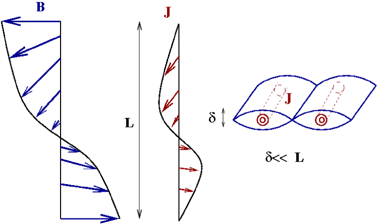
Figure 3: Development of a tearing mode. Initial configuration consists of a current layer in which magnetic field rotates by $\pi$ radians. Current is flowing along magnetic field. A thin current sheet forms due to development of tearing mode. Magnetic islands form inside the resistive current sheet.

Tearing mode is quite complicated (Furth et al. 1963, White 1983, Fig. 3). The basic physical processes leading to development of tearing mode are the following. A current sheet may be represented as a set of elementary current filaments. Since current filaments attract each other the current sheet is unstable against pairing of current filaments. For sufficiently narrow current sheets the energy released by pairing of currents is more than the energy spent to maintain perturbed magnetic field - tearing mode has negative energy, so that its dissipation should increase its amplitude leading to dissipation. Magnetic islands form in plasma as a result of the development of tearing mode. Typical time scale for the development of the tearing mode is intermediate between a short Alfvén and long resistive time scale.

2 Resistive force-free electrodynamics

Under force-free approximation it is assumed that the plasma dynamics is completely controlled by magnetic field. The validity of this approximation requires $b^{2}\gg\rho c^{2}$, where $b$ and $\rho$ are plasma rest-frame magnetic field and density. It is assumed that the plasma provides currents and charge densities required by the dynamics of electro-magnetic fields, but these current carry no inertia.

In addition to being magnetically-dominated, microscopic plasma processes, like particle collisions or plasma turbulence, may contribute to resistivity and thus make plasma non-ideal. Resistivity will result in the decay of currents supporting the magnetic field; this, in tern, will influence the plasma dynamics. We wish to explore how the decay of inertialess currents will affect the dynamics of the system. We assume that plasma resistivity can be represented by phenomenological parameter $\eta$. To calculate $\eta$ from microscopical principles one needs to take the particle dynamics into account and thus go beyond the inertialess approximation. The answer will depend on the types of current-carrying particle (e.g. electron-ion or pair plasma) and on the dominant type of scattering (e.g. particle-particle, particle-wave or particle-wave-particle). We wish to avoid this complication by introducing a macroscopic parameter $\eta$. We also assume that the dissipated energy of the magnetic field leaves the system, e.g. in a form of radiation. If this was not the case, the particle pressure would build up to equipartition breaking the force-free assumption.

Strictly speaking, inclusion of resistivity violates the force-free condition since non-zero resistance implies that there is extra force acting on charge carries. Still, in strongly magnetized plasmas the resistive forces act only along the direction of the magnetic field, while the dynamics transverse to the magnetic field remains unaffected, given by the force-free conditions (12). What distinguishes resistive and ideal cases is the way the current is related to the field (Ohm’s law). It is in this sense that we will use the term resistive force-free electro-dynamics.

The procedure described above is not entirely consistent in case of relativistic plasmas. The reason is that in an ideal force-free plasma the velocity along the field is not defined. Since plasma resistivity must be defined in the plasma rest-frame this creates a principal ambiguity. Note, that in case of non-relativistic force-free plasma such ambiguity does not appear: it is possible to write a self-consistent system of equations describing evolution of non-relativistic resistive force-free plasma (Chandrasekhar & Kendall 1957, Low 1973). In the non-relativistic plasma evolution of resistive force-free fields proceeds in a self-similar ways: magnetic fields keep their configuration while changing in magnitude. In a process of doing so small electric fields and charge densities develop, whose dynamical contribution is neglected in the non-relativistic case. In relativistic case we cannot neglect these effects so that evolution force-free resistive fields becomes much more complicated.

2.1 Ohm’s law in magnetically-dominated plasma

Relativistic form of Ohm’s law in magnetized plasma may be formally written assuming that in the plasma rest frame the current is proportional to the electric field. Several attempts have been made to derive Ohm’s law in relativistic plasma; none seem completely satisfactory so far. Blackman and Field (1993) assumed that there exists a frame where charge density, momentum density and velocity flux density are all zero, but in a general case the plasma may be charged in its rest frame (defined, for example, as a frame where momentum density is zero). Gedalin (1996) wrote expressly covariant form of the relativistic Ohm’s law in isotropic plasma. In strong magnetic field we expect that transverse and parallel (with respect to magnetic field) conductivities are different, so that conductivity becomes a tensor:

$$F^{ik}U_{k}=\eta^{ik}\left(\delta_{k}^{l}-U_{k}U^{l}\right)j_{l}$$ (1)

where $\eta^{ik}$ is a conductivity tensor. To find an expression for $\eta^{ik}$ we need to consider particle dynamics taking into account particle-particle interaction. Derivation of a general expression for $\eta^{ik}$ is a project worth a separate paper. Here we give simplified expressions for $\eta^{ik}$ in case of strongly magnetized plasma.

To derive Ohm’s law in force-free plasma, which assumes a one-fluid description, we need to define the plasma rest-frame. In relativistic plasma the choice of plasma rest-frame is not unique (e.g. de Groot et al. 1980). In a force-free plasma the ambiguity of the rest frame is partially removed: though the motion along the magnetic field still remains undefined, the motion of particles across the magnetic field consists only of an electric drift

$${\bf v}_{\perp}={{\bf E}_{\perp}\times{\bf B}\over B^{2}},$$ (2)

which allows one to introduce a plasma frame (up to a boost along the field), as a frame where drift velocity vanishes. Since both species drift with the same velocity, there is no relative motion of particles across the field and thus there is no resistivity across the magnetic field (the current across the field is due to exclusively different charge densities of two species). An alternative way of reasoning supporting this conclusion is that in force-free plasma there is no current across the field in the plasma rest-frame, where resistivity should be defined.

Thus, under force-free approximation the resistive effects affect only the motion along the field. To derive the corresponding Ohm’s law we introduce a four-dimensional magnetic field vector

$$b_{i}=\ast F_{ik}U^{k}$$ (3)

where $\ast F_{ik}$ is a dual electro-magnetic tensor. If ${\bf B}$ denotes the plasma rest frame magnetic field, then $B_{i}=\{0,{\bf B}\}$ and

$$b_{i}=\gamma\{({\bf v}\cdot{\bf B}),{\bf B}\}$$ (4)

Convolving eq. (1) with $b_{i}$ we find

$$F^{ik}U_{k}\ast F_{il}U^{l}=\eta^{ik}b_{i}\left(\delta_{k}^{l}-U_{k}U^{l}\right)j_{l}$$ (5)

Since we expect that in the strongly magnetized plasma resistivity is important only along the field, we assume

$$\eta^{ik}=\eta{b^{i}b^{k}\over b^{2}}$$ (6)

We find then

$$F^{ik}U_{k}\ast F_{il}U^{l}=\eta(jb)=\eta\ast F_{il}U^{l}j^{i}$$ (7)

since $(bU)=0$. Equation (7) gives Ohm’s law in force-free plasma. In 3-D notations this gives

$$\gamma^{2}\left(({\bf E}\cdot{\bf v})({\bf B}\cdot{\bf v})-({\bf E}+{\bf v}\times{\bf B})\cdot({\bf B}+{\bf v}\times{\bf E})\right)=\eta\gamma\left(j_{0}({\bf B}\cdot{\bf v})-({\bf J}\cdot{\bf B})\right)$$ (8)

Next we separate electric fields and velocity into components along and across the magnetic field, ${\bf E}={\bf E}_{\parallel}+{\bf E}_{\perp}$, ${\bf v}={\bf v}_{\parallel}+{\bf v}_{\perp}$ with ${\bf v}_{\perp}={\bf E}_{\perp}\times{\bf B}/B^{2}$. Then eq. (8) simplifies

$$E_{\parallel}\left(v_{\parallel}^{2}-1\right)={\eta\over\gamma}\left(j_{0}v_{\parallel}-J_{\parallel})\right)$$ (9)

Since the velocity along the field cannot be specified within the framework of force-free plasma we chose $v_{\parallel}=0$. The ambiguity for the choice of $v_{\parallel}$ stems from the fact that the force-free approximation cannot in principle describe the plasma dynamics along the magnetic fields – however strong the field is, it does not affect particle motion align the field, so that one must use full MHD equations. For example, in a frame-work of two-fluid hydrodynamics there are two equations of motion describing the dynamics of each species along the field. The difference of these equations gives the generalized Ohm’s law. The sum gives the equation of bulk motion of plasma due to the influence of external fields. Since we neglect the Poynting flux associated with the bulk motion this equation is neglected. Then the choice of parallel velocity becomes just a choice of coordinate system.

In spite of limitations concerning the parallel dynamics of plasma there is a number of relevant problems where one can neglect the plasma dynamics along the field either because the variation in that direction are small or because of a symmetry of the system (e.g. if magnetic field is directed along a cyclic variable).

Setting $v_{\parallel}=0$ in (9) we find

$$({\bf E}\cdot{\bf B})={\eta\over\gamma}({\bf J}\cdot{\bf B})$$ (10)

The factor $\gamma=1/\sqrt{1-({\bf E}\times{\bf B}/B^{2})^{2}}$ comes from the Lorenz transformation of the electric field to the plasma rest frame ($J_{\parallel}$ is invariant under Lorentz transformation along the direction orthogonal to magnetic field). Reinstating the transverse current, we find Ohm’s law in relativistic force-free electro-dynamics

$${\bf J}={{\rm\,div\,}{\bf E}({\bf E}\times{\bf B})\over B^{2}}+{1\over\eta\sqrt{1-\left({({\bf E}\times{\bf B})\over B^{2}}\right)^{2}}}{({{\bf E}\cdot{\bf B}}){\bf B}\over B^{2}}$$ (11)

Taking a vector product with ${\bf B}$ in Ohm’s law we find a cross-field dynamical equation

$${\bf J}\times{\bf B}+{\rm\,div\,}{\bf E}\left({\bf E}-{({\bf E}\cdot{\bf B})\over B^{2}}{\bf B}\right)\equiv{\bf J}\times{\bf B}+{\bf E}_{\perp}{\rm\,div\,}{\bf E}=0$$ (12)

This generalizes the force-free condition for resistive plasma.

2.2 Equations of resistive force-free electro-dynamics

The resistive force-free electrodynamics may be derived from RMHD in the limit of vanishing plasma inertia $w,\,p,\,\rho\rightarrow 0$ and by reinstating electric field

$${\bf E}={\bf E}_{\parallel}+{\bf E}_{\perp}={({\bf E}\cdot{\bf B}){\bf B}\over B^{2}}-{\bf v}\times{\bf B}.$$ (13)

In a force-free formulation the plasma velocity is defined only up to an arbitrary Lorenz boost along the magnetic field direction. The velocity across the magnetic field is just the electro-magnetic drift velocity ${\bf E}\times{\bf B}/B^{2}$. The dynamical equations are Maxwell equations and Ohm’s law (11)

$$\dot{{\bf B}}=-{\rm curl\,}{\bf E}\mbox{}$$

$$\dot{{\bf E}}={\rm curl\,}{\bf B}-{\bf J}$$ (14)

(we use a system of units with the speed of light set to unity; we also incorporate the coefficient $4\pi$ into definitions of currents and charge densities).

Resistive force-free electrodynamics is more complicated than its non-relativistic analogue. In the non-relativistic case currents can be expressed from the second Maxwell equation and electric field can be eliminated from Ohm’s law. In relativistic case this is impossible - the best that we can do is to eliminate the current from Ohm’s law and solve Maxwell equations for a ${\bf B}$ and ${\bf E}$ (this is a system of 5 equations since the constraint ${\rm\,div\,}{\bf B}=0$ must be satisfied at all times). Resistive force-free electrodynamics is also more complicated than the ideal one. In ideal force-free electrodynamics the condition ${\bf E}\cdot{\bf B}=0$ reduced a number of equations to 4 (Komissarov 2002, Lyutikov & Blandford 2003). In addition, in ideal case the second electro-magnetic invariant is always larger than 0, $B^{2}-E^{2}>0$, which implies that there is a reference frame where electric field is equal to 0. In case of resistive electrodynamics $B^{2}-E^{2}$ may be smaller than zero, which implies an electric field in the plasma rest frame.

The form of Ohm’s law (11) may not be appropriate for some applications: for example, the transition to the ideal case ($\eta\rightarrow 0$) leave us with no conditions on the current. To make the transitions from the resistive to the ideal case clearer we combine Maxwell equations by taking scalar products with ${\bf B}$ and ${\bf E}$

$$({\bf J}\cdot{\bf B})=({\bf B}\cdot\nabla\times{\bf B}-{\bf E}\cdot\nabla\times{\bf E}){\bf B}-\partial_{t}\left({\bf E}\cdot{\bf B}\right)$$ (15)

The term ${\bf B}\cdot\nabla\times{\bf B}$ is called current helicity, the corresponding term involving electric fields does not have a name (it does not appear in non-relativistic analysis).

Using the Ohm’s law (11) we can eliminate $\left({\bf E}\cdot{\bf B}\right)$ from (15)

$$({\bf J}\cdot{\bf B})+\partial_{t}\left(\eta\sqrt{1-\left(({\bf E}\times{\bf B})/B^{2}\right)^{2}}({\bf J}\cdot{\bf B})\right)=({\bf B}\cdot\nabla\times{\bf B}-{\bf E}\cdot\nabla\times{\bf E}){\bf B}$$ (16)

which gives an alternative form of Ohm’s law. This form has an advantage that, unlike eq. (11), it clearly shows how to make a transition to the ideal case.

Given Ohm’s law (11) we can write down the basic law of energy and momentum conservation in resistive force-free electro-dynamics:

$${1\over 2}\partial_{t}(B^{2}+E^{2})={\rm\,div\,}{\bf E}\times{\bf B}-{1\over\eta\sqrt{1-\left({({\bf E}\times{\bf B})\over B^{2}}\right)^{2}}}{({{\bf E}\cdot{\bf B}})^{2}\over B^{2}}\mbox{}$$

$$\partial_{t}({\bf E}\times{\bf B})={\rm curl\,}{\bf B}\times{\bf B}-{\rm curl\,}{\bf E}\times{\bf E}-{\bf J}\times{\bf B}=\mbox{}$$

$${\rm curl\,}{\bf B}\times{\bf B}-{\rm curl\,}{\bf E}\times{\bf E}+{\rm\,div\,}{\bf E}\left({\bf E}-{({\bf E}\cdot{\bf B})\over B^{2}}{\bf B}\right)$$ (17)

In ideal plasma, $\eta=0$, Ohm’s law gives ${\bf E}\cdot{\bf B}=0$. This condition plus the Maxwell equations (14) are then sufficient to express the current in terms of fields,

$${\bf J}={({\bf E}\times{\bf B})\nabla\cdot{\bf E}+({\bf B}\cdot\nabla\times{\bf B}-{\bf E}\cdot\nabla\times{\bf E}){\bf B}\over B^{2}}$$ (18)

while eq. (12) gives

$${\bf J}\times{\bf B}+{\bf E}{\rm\,div\,}{\bf E}=0$$ (19)

Equations (14) and (18) (or (19)) are then the equations of ideal force-free electrodynamics (Uchida 1997, Gruzinov 1999, Komissarov 2002, Lyutikov & Blandford 2003).

2.3 Applicability of force-free approximation

Force-free electro-dynamics assumes that inertia of plasma is negligible. This approximation is bound to break down for very large effective plasma velocities, when electric field becomes too close in value to magnetic field, $E\rightarrow B$. The condition that inertia is negligible is equivalent to the condition that the effective plasma four-velocity, $u\sim E/(B\sqrt{1-(E/B)^{2}})$, is smaller that the Alfvén four-velocity in plasma. Assume that in the plasma rest frame the ratio of magnetic energy density to plasma energy density (which may include both rest mass energy density and internal energy) is $\sigma$. In a strongly magnetized plasma $\sigma\gg 1$ (in a force-free plasma $\sigma$ is assumed to be infinite). Then the Alfvén wave phase velocity and the corresponding Lorentz factor are (e.g. Kennel & Coroniti 1984, Lyutikov & Blandford 2003)

$$u_{A}^{2}={\sigma}$$ (20)

This puts an upper limit on the value of electric fields consistent with force-free approximation

$${B^{2}-E^{2}\over E^{2}}\gg{1\over\sigma}$$ (21)

3 Relativistic Current Sheets

3.1 Ideal Force-free Current Sheets

Since we are interested in the stability of weakly resistive configurations, we first consider steady state planar solution of the ideal force-free electrodynamics (eqns. (14) and (18)). Assume that magnetic field lays in the $x-y$ plane, $B_{z}=0$, and that all quantities dependent only on $z$. Then from the first Maxwell equation we find that $E_{x},\,E_{y}\sim{\rm const}$. The $x$ and $z$ components of the ${\rm curl\,}{\bf B}={\bf J}$ equation then give ($y$ component is the same as $x$)

$$\partial_{z}\left(B_{x}^{2}+B_{y}^{2}-E_{z}^{2}\right)=0\mbox{}$$

$$\left(B_{y}E_{x}-B_{x}E_{y}\right)\partial_{z}E_{z}=0$$ (22)

In addition, for ideal plasma condition ${\bf E}\cdot{\bf B}=0$ requires

$$B_{x}E_{x}+B_{y}E_{y}=0$$ (23)

Below we discuss several possible solutions of these equations. The two main types of current sheet equilibrium are the current sheets (when the electric field is zero and there is no motion of plasma) and shear layer, where non-zero electric fields lead to plasma motion in the plane of the current sheet or into it, creating magnetic and velocity-sheared configurations.

1. Crossed constant electric and magnetic fields. We assume that the components of the electric field in the plane of the sheets are non-zero, $E_{x}E_{y}\neq 0$ and, in addition, $E_{z}\sim{\rm const}$. This case corresponds to plasma in constant electric and magnetic fields moving with velocities

   $${\bf V}=\left\{{E_{z}\over B_{0}\sqrt{1+E_{y}^{2}/E_{x}^{2}}},-{E_{y}E_{z}\over B_{0}E_{x}\sqrt{1+E_{y}^{2}/E_{x}^{2}}},{E_{x}^{2}-E_{y}^{2}\over B_{0}E_{x}\sqrt{1+E_{y}^{2}/E_{x}^{2}}}\right\}$$ (24)

   (in Cartesian coordinates $x,y,z$). By Lorentz transformation electric fields can be completely eliminated, so that in the plasma rest frame ${\bf E}=0$.

2. Sheared force-free layer. Assuming $E_{x}=E_{y}=0$, $E_{z}\neq 0$ we find

   $$B_{x}^{2}+B_{y}^{2}-E_{z}^{2}=B_{0}^{2}$$ (25)

   where $B_{0}$ is some constant. There are two interesting types of equilibrium here. First is a sheared $B_{x}$ field in a constant guiding field $B_{y}=B_{0}/U_{0}$ ($U_{0}$ is some constant).

   $${\bf B}=B_{0}\left\{\tanh z/L,{1\over U_{0}},0\right\}\mbox{}$$

   $${\bf E}=B_{0}\left\{0,0,\tanh z/L\right\}\mbox{}$$

   $${\bf J}={B_{0}\over L}\left\{0,{\rm\,sech\,}^{2}z/L,0\right\}\mbox{}$$

   $$\rho_{e}=-{B_{0}\over L}{\rm\,sech\,}z/L\tanh z/L\mbox{}$$

   $${\bf V}=\left\{{U_{0}\tanh z/L\over 1+U_{0}^{2}\tanh^{2}z/L},-{U_{0}^{2}\tanh^{2}z/L\over 1+U_{0}^{2}\tanh^{2}z/L},0\right\}\mbox{}$$

   $$v^{2}={U_{0}^{2}\tanh^{2}z/L\over 1+U_{0}^{2}\tanh^{2}z/L},\,\gamma^{2}=1+U_{0}^{2}\tanh^{2}z/L\mbox{}$$

   $${\bf P}=B_{0}^{2}\left\{{1\over U_{0}}\tanh z/L,\tanh^{2}z/L\right\}$$ (26)

   where $L$ is a characteristic width of the layer, ${\bf P}$ is a Poynting flux. Thus, there is a Poynting flux of electro-magnetic energy along the current layer. At the different side of the current layer $P_{y}$ changes sing, while $P_{x}$ remains the same. (Fig. 1). The layer is sheared both in $x$ and $y$ direction. On the different sides of the current layer the plasma is streaming in opposite direction along the $x$, with a four velocity at infinity reaching $u_{x}=\pm U_{0}/\sqrt{1+U_{0}^{2}}$, while along the $y$ direction the plasma is streaming in the same direction on both sides of the layer, reaching at infinity $u_{y}=-U_{0}^{2}/\sqrt{1+U_{0}^{2}}$.

   Another possible type of layer is a sheared and rotating magnetic field, (Blandford, private communication)

   $${\bf B}=B_{0}\left\{\tanh z/L,\sqrt{2}{\rm\,sech\,}z/L,0\right\}\mbox{}$$

   $${\bf E}=B_{0}\left\{0,0,{\rm\,sech\,}z/L\right\}\mbox{}$$

   $${\bf J}={B_{0}\over L}\left\{\sqrt{2}{\rm\,sech\,}z/L\tanh z/L,{\rm\,sech\,}^{2}z/L,0\right\}\mbox{}$$

   $$\rho_{e}=-{B_{0}\over L}{\rm\,sech\,}z/L\tanh z/L\mbox{}$$

   $${\bf V}=\left\{-{\sqrt{2}\over 1+\cosh^{2}z/L},{\sinh z/L\over 1+\cosh^{2}z/L},0\right\}\mbox{}$$

   $$v^{2}={1\over 1+\cosh^{2}z/L},\,\gamma^{2}=1+{\rm\,sech\,}^{2}z/L\mbox{}$$

   $${\bf P}=\left\{-\sqrt{2}{\rm\,sech\,}^{2}z/L,{\rm\,sech\,}z/L\tanh z/L,0\right\}$$ (27)

   (Fig. 2).

3. Magnetic rotation discontinuity ${\bf E}=0$. In this case we find $B^{2}=B_{0}^{2}$, so that magnetic field rotates keeping its absolute value constant (Fig. 3). This case will be our primary interest.

Finally we note, that since ideal electro-dynamics supports only two types of waves (luminal fast modes and subluminal Alfvén modes), the current sheets discussed above are nothing else but Alfvén waves considered in some preferred frame of reference (Komissarov 2002). Then the instability considered below are related to the instabilities of 1-D dissipative Alfvén waves (we thank S. Komissarov for pointing this out).

3.2 Resistive Force-free Current Sheets

In a strongly resistive media one may seek stationary solutions of the equation of resistive electro-dynamics (14, 11), assuming that resistive terms are important everywhere (in a way similar to important works of Low (1973) for non-relativistic plasma). Assuming a sheared magnetic field field configuration with $E_{z}=0$ we find

$$B_{y}^{\prime}=-{1\over\eta}{B_{x}({\bf E}\cdot{\bf B})\over\sqrt{B^{2}-(E_{y}B_{x}-B_{y}E_{x})^{2}}}\mbox{}$$

$$B_{x}^{\prime}={1\over\eta}{B_{y}({\bf E}\cdot{\bf B})\over\sqrt{B^{2}-(E_{y}B_{x}-B_{y}E_{x})^{2}}}$$ (28)

From which it follows that $B^{2}={\rm const}$. Assuming $B_{x}=\cos\phi(z),B_{y}=\sin\phi(z)$ and setting without loss of generality $E_{y}=0$ we find equation for $\phi$:

$$\partial_{z}\phi=-{1\over\eta}{E_{x}\cos\phi\over\sqrt{1-E_{x}^{2}\sin^{2}\phi}}$$ (29)

Which can be integrated to give an implicit dependent $\phi(z)$:

$${E_{x}z\over B_{0}\eta}=-{E_{x}\over B_{0}}{\rm arcsin}({E_{x}\over B_{0}}\sin\phi)-{\sqrt{1-(E_{x}/B_{0})^{2}}\over 2}\ln{\cal A}\mbox{}$$

$${\cal A}=\left({1\over\cos^{2}\phi}\left(1+\left(1-2\left({E_{x}\over B_{0}}\right)^{2}\right)\sin^{2}\phi+2\sqrt{1-\left({E_{x}\over B_{0}}\right)^{2}}\sin\phi\sqrt{1-\left({E_{x}\over B_{0}}\right)^{2}\sin^{2}\phi}\right)\right)$$ (30)

It describes a inflow of plasma into resistive current layer. For small $(E_{x}/B_{0})\rightarrow 0$ this gives

$$\phi=-\tanh{E_{x}z\over B_{0}\eta}$$ (31)

which corresponds to the Low (1973) solution

$$B_{x}=B_{0}{\rm\,sech\,}{E_{x}\over B_{0}}{z\over\eta}\mbox{}$$

$$B_{y}=-B_{0}\tanh{E_{x}\over B_{0}}{z\over\eta}\mbox{}$$

$$v_{z}=-{E_{x}\over B_{0}}\tanh{E_{x}\over B_{0}}{z\over\eta}$$ (32)

Application of this solution to astrophysical plasmas suffers from the same problem as the original Low’s solution: the diffusion time scales are much longer than the time scales of interest. We suspect (though did not show it) that the relativistic solutions (30) is unstable to small perturbations which would lead to electric current singularity. This brings us to the main part of the paper - development of resistive current sheets in a relativistic force-free plasma.

4 Tearing mode stability of rotational discontinuities

A standard method in describing the evolution of tearing mode is similar to the boundary layer problem . It involves a separation of a current layer into a ”bulk”, where derivatives are small and resistivity is not important, and a narrow ”boundary layer” where derivatives and resistivity may be large. Two different approximations are done in each layer - ideal and weakly varying plasma in the bulk and a narrow resistive sublayer (Fig. 3). Two solutions should be matched continuously.

In this section we investigate a resistive stability of a relativistic current layer. We assume that initially the electric field is zero, so that the magnetic field while remaining constant in magnitude rotates over some angle (Section 3.1), which we chose to be $\pi$ radians for simplicity.

Assume that a current layer has a width $L$. Since $B^{2}=const$, a possible form of the unperturbed magnetic field is

$$B_{0,x}=B_{0}{z\over L}\mbox{}$$

$$B_{0,y}=B_{0}\sqrt{1-\left({z\over L}\right)^{2}}$$ (33)

Next we investigate stability of such current layer to small perturbations.

4.1 Stability of resistive force-free current sheet

In this main section of the paper we investigate the stability properties of a planar resistive current sheet. We assume that in the bulks of the plasma resistivity is small, so that initial configuration is described by an ideal current sheet in which magnetic field remains planar ($B_{z}=0$) and rotates over some angle $B^{2}=B_{0}^{2}$, while electric field is zero $E=0$. Formally we should start with resistive solution (30) with has non-zero velocity of plasma into the current layer, but for large scale current that resistive inflow velocity is negligible.

Consider small fluctuations of the electro-magnetic fields and current

$${\bf B}={\bf B}_{0}+{\bf b}\mbox{}$$

$${\bf E}={\bf e}\mbox{}$$

$${\bf J}={\bf J}_{0}+{\bf j}$$ (34)

Assume that the perturbations vary as $\exp\{i(\omega t-k_{x}x-k_{y}y)\}$. Then eqns (14), (16) and (12) give

$$b_{z}\omega-({\bf k}\times{\bf e})_{z}=0\mbox{}$$

$$i({\bf k}\cdot{\bf b})-\partial_{z}({\bf k}\times{\bf e})_{z}=0\mbox{}$$

$$e_{z}k^{2}+\omega({\bf k}\times{\bf b})_{z}\omega-i\partial_{z}({\bf k}\cdot{\bf e})=0\mbox{}$$

$$({\bf k}\cdot{\bf j})+i\omega({\bf k}\cdot{\bf e})+\partial_{z}({\bf k}\times{\bf b})_{z}=0\mbox{}$$

$$b_{z}k^{2}+i({\bf k}\times{\bf j})_{z}-\omega({\bf k}\times{\bf e})_{z}-i\partial_{z}({\bf k}\cdot{\bf b})=0\mbox{}$$

$$j_{z}+i(({\bf k}\times{\bf b})_{z}+\omega e_{z})=0\mbox{}$$

$$({\bf B}_{0}\cdot{\bf e})-\eta(({\bf B}_{0}\cdot{\bf j})-({\bf B}_{0}\cdot{\bf b})H)=0\mbox{}$$

$$j_{z}+b_{z}H=0$$ (35)

where $H=(B_{x}\partial_{z}B_{y}-B_{y}\partial_{z}B_{x})/B_{0}^{2}$ is a normalized current vorticity of the initial state and ${\bf k}=\{k_{x},k_{y},0\}$.

We can readily eliminate current, $({\bf k}\times{\bf j})_{z},\,({\bf k}\cdot{\bf j}),\,j_{z}$, as well as z-components of electric and magnetic field fluctuations $e_{z}$ and $b_{z}$. After some rearrangements the equations involving fluctuations of $x$- and $y-$ components of electric and magnetic fields become

$$i({\bf k}\cdot{\bf b})-\partial_{z}({\bf k}\times{\bf e})_{z}=0\mbox{}$$

$$i\omega({\bf k}\times{\bf b})_{z}\left(1-{\omega^{2}\over k^{2}}\right)-H\omega({\bf k}\times{\bf e})_{z}-{\omega^{2}\over k^{2}}\partial_{z}({\bf k}\cdot{\bf e})=0\mbox{}$$

$$({\bf B}_{0}\cdot{\bf e})-\eta\left(i({\bf k}\times{\bf B}_{0})_{z}({\bf k}\times{\bf e})_{z}-2\omega H({\bf B}_{0}\cdot{\bf b})-\omega\partial_{z}({\bf B}_{0}\times{\bf b})_{z}\right)=0\mbox{}$$

$$i({\bf k}\cdot{\bf B}_{0})({\bf k}\times{\bf e})_{z}-i\omega^{2}({\bf B}_{0}\times{\bf e})_{z}+\partial_{z}({\bf B}_{0}\cdot{\bf b})=0$$ (36)

From which we can eliminate magnetic fields

$$({\bf B}_{0}\cdot{\bf b})=-i\left({({\bf k}\cdot{\bf B}_{0})\partial_{z}({\bf k}\times{\bf e})_{z}\over k^{2}\omega}+{({\bf k}\times{\bf B}_{0})_{z}\left(Hk^{2}({\bf k}\times{\bf e})_{z}+\omega^{2}\partial_{z}({\bf k}\cdot{\bf e})\right)\over k^{2}\omega(k^{2}-\omega^{2})}\right)\mbox{}$$

$$({\bf B}_{0}\times{\bf b})_{z}=i\left({({\bf k}\times{\bf B}_{0})_{z}\partial_{z}({\bf k}\times{\bf e})_{z}\over k^{2}\omega}-{({\bf k}\cdot{\bf B}_{0})\left(H({\bf k}\times{\bf e})_{z}+\omega^{2}/k^{2}\partial_{z}({\bf k}\cdot{\bf e})\right)\over\omega(k^{2}-\omega^{2})}\right)$$ (37)

This, with corresponding equations for electric fields

$$({\bf B}_{0}\cdot{\bf e})-\eta\left(i({\bf k}\times{\bf B}_{0})_{z}({\bf k}\times{\bf e})_{z}-2H\omega({\bf B}_{0}\cdot{\bf b})-i\omega^{2}({\bf B}_{0}\cdot{\bf e})-\omega\partial_{z}({\bf B}_{0}\times{\bf b})_{z}\right)=0\mbox{}$$

$$i({\bf k}\cdot{\bf B}_{0})({\bf k}\times{\bf e})_{z}-i\omega^{2}({\bf B}_{0}\times{\bf e})_{z}+\partial_{z}({\bf B}_{0}\cdot{\bf b})=0$$ (38)

is where we stop the general approach.

4.2 Ideal current layer

In the bulk of the plasma we can neglect resistivity so that the dynamics of the current layer is governed by equations (14,18). In this section we investigate stability of an ideal force-free current sheet to small perturbation (see also Gruzinov 1999).

For ideal plasma $\eta=0$, we find

$$\partial_{z}\left(F\partial_{z}{e_{y}\over B_{x}\omega}\right)+{e_{y}\over B_{x}\omega}F(\omega^{2}-k^{2})=0$$ (39)

Or, returning to the definition of $b_{z}$

$$\partial_{z}\left(F\partial_{z}{b_{z}\over({\bf B}_{0}\cdot{\bf k})}\right)+{b_{z}\over({\bf B}_{0}\cdot{\bf k})}F(\omega^{2}-k^{2})=0$$ (40)

where $F=({\bf B}_{0}\cdot{\bf k})^{2}-\omega^{2}B_{0}^{2}$. Equation (40) describes stability properties of an ideal relativistic force-free current sheet. A quick examination shows that similar to the non-relativistic case points $({\bf B}_{0}\cdot{\bf k})=0$ is a special point of the equation. Fluctuation of the magnetic field $b_{z}$ diverge at these surfaces creating current sheets.

Consider fluctuations near the surfaces $({\bf B}_{0}\cdot{\bf k})=0$. Assume that $B_{x}$ becomes zero at $z=0$; then, neglecting variations in $y$ direction, $k_{y}\rightarrow 0$ and introducing displacement $\xi=b_{z}/B_{x}k_{x}$ we find

$$\left(B_{x}^{2}k_{x}^{2}-B_{0}^{2}\omega^{2}\right)\left(\xi(\omega^{2}-k_{x}^{2})+\partial_{z}^{2}\xi\right)+2B_{x}k_{x}^{2}\partial_{z}\xi\partial_{z}B_{x}$$ (41)

which can be further simplified

$$(\hat{k}_{x}^{2}-\hat{\omega}^{2})\left(\hat{B}_{x}^{2}\hat{k}_{x}^{2}-\hat{\omega}^{2}\right)\xi(Z)-\partial_{Z}^{2}\xi(Z)$$ (42)

where

$$\hat{k}_{x}=k_{x}L\mbox{}$$

$$\hat{\omega}=\omega L\mbox{}$$

$$\hat{B}_{x}={B_{x}\over B_{0}}\mbox{}$$

$$\hat{z}={z\over L}\mbox{}$$

$$Z=\int{1\over\hat{k}_{x}^{2}\hat{B}_{x}^{2}-\hat{\omega}^{2}}d\hat{z}$$ (43)

For example, for a linear $\hat{B}_{x}=\hat{z}$, we find $Z=-{\rm arctan}(\hat{k}_{x}\hat{z}/\hat{\omega})/(\hat{k}_{x}\hat{\omega})$. Then eq. (42) gives

$$\hat{\omega}^{4}(\hat{k}_{x}^{2}-\hat{\omega}^{2}){\rm\,sech\,}^{2}(\hat{k}_{x}\hat{\omega}Z)\xi-\partial_{Z}^{2}\xi(Z)=0$$ (44)

which has a form of a non-linear oscillator.

General solution of Eq. (44) is quite complicated. Its dependence on $\hat{\omega}$ shows that variations of the field have electro-magnetic structure (as oppose to purely magnetostatic variations in the non-relativistic case). We expect that typical growth rates will be small $\hat{\omega}\ll\hat{k}_{x}$, so that we can neglect the electro-magnetic corrections by setting $\hat{\omega}\rightarrow 0$. This will have to be checked a posteriori. This limit corresponds to non-relativistic approximation, so that the relations (45-48) coincide with the familiar relations for the non-relativistic tearing mode.

In the limit $\hat{\omega}\rightarrow 0$ eq. (41) gives for $\hat{B}_{x}=\hat{z}$ when $|\hat{z}|<1$ and $\hat{B}_{x}=1$ for $|\hat{z}|>1$

$$\xi=\left\{\begin{array}[]{cc}C_{1}{\cosh\hat{k}_{x}\hat{z}\over\hat{z}}+C_{2}{\sinh\hat{k}_{x}\hat{z}\over\hat{z}}&\mbox{ if $|\hat{z}|<1$ }\\ C_{0}\exp\{-\hat{k}_{x}|\hat{z}|\}&\mbox{ if $|\hat{z}|>1$}\end{array}\right.$$ (45)

where we have chosen a solution which is decaying as $|\hat{z}|\rightarrow\infty$. Matching the two solutions at $|\hat{z}|=1$ gives

$$C_{1}={C_{0}\over 2\hat{k}_{x}}\left(2\hat{k}_{x}-1+\exp\{-2\hat{k}_{x}\}\right)\mbox{}$$

$$C_{2}={C_{0}\over 2\hat{k}_{x}}\left(1-2\hat{k}_{x}+\exp\{-2\hat{k}_{x}\}\right)$$ (46)

Given a solution for $\xi$ we can find magnetic field fluctuation

$${b_{z}\over B_{0}}=\hat{B}_{x}\hat{k}_{x}\xi=\hat{k}_{x}\left(C_{1}\cosh\hat{k}_{x}\hat{z}+C_{2}\sinh\hat{k}_{x}\hat{z}\right)$$ (47)

Magnetic field is continuous at $\hat{z}=0$ but its derivative experiences a jump

$$\Delta\equiv\left[{\partial_{\hat{z}}b_{z}\over b_{z}}\right]={2C_{2}\hat{k}_{x}\over C_{1}}\approx{2\over\hat{k}_{x}}\mbox{, for $\hat{k}_{x}\ll 1$}$$ (48)

This means that there is current sheet forming at $\hat{z}=0$.

4.3 Structure of resistive sublayer

To study the structure of the resistive sublayer we make several approximations for equations (37-38). First, we neglect variations along the $y$-axis, $k_{y}\rightarrow 0$. We find then

$$e_{x}B_{x}+e_{y}B_{y}+{\eta\over\Gamma}\left(e_{y}\left(B_{y}(H^{2}+k_{x}^{2})+B_{x}\partial_{z}H\right)+2B_{x}H\partial_{z}e_{y}-B_{y}\partial_{z}^{2}e_{y}+\right.\mbox{}$$

$$\left.{\Gamma^{2}\over k_{x}^{2}+\Gamma^{2}}\left((B_{x}e_{x}+B_{y}e_{y})(k_{x}^{2}+\Gamma^{2})+(B_{y}H^{2}+B_{x}\partial_{z}H)e_{y}+H(B_{y}\partial_{z}e_{x}+B_{x}\partial_{z}e_{y})+B_{x}\partial_{z}^{2}e_{x}\right)\right)=0\mbox{}$$

$$e_{y}\left(B_{x}(k_{x}^{2}-H^{2})-B_{y}\partial_{z}H\right)-B_{x}\partial_{z}^{2}e_{y}+\mbox{}$$

$${\Gamma^{2}\over k_{x}^{2}+\Gamma^{2}}\left((e_{y}B_{x}-B_{y}e_{x})(k_{x}^{2}+\Gamma^{2})+e_{y}(B_{x}^{2}H^{2}+B_{y}\partial_{z}H)+H(B_{x}\partial_{z}e_{x}+B_{y}\partial_{z}e_{y})+B_{y}\partial_{z}^{2}e_{x}\right)=0$$ (49)

where $\Gamma=-i\omega$.

We expect that the width of the resistive layer, $\sim\epsilon L$ is much smaller than the width of the current layer $L$, $\epsilon\ll 1$. We then expand system (49) near $z\sim\epsilon$ by introducing $\zeta=\epsilon z/L$.

For $\epsilon\ll 1$ we find

$$e_{y}-e_{x}\zeta\epsilon-\hat{\eta}{\partial_{\zeta}^{2}e_{y}\over\epsilon^{2}}=0\mbox{}$$

$$\zeta\left(e_{y}\hat{k}_{x}^{2}\epsilon^{2}-{\partial_{\zeta}^{2}e_{y}}\right)+{\hat{\Gamma}^{2}\over\hat{k}_{x}^{2}}\left({\partial_{z}^{2}e_{x}\over\epsilon}-{\partial_{\zeta}(\zeta\partial_{\zeta}e_{y})\over\zeta}\right)=0$$ (50)

where $\hat{\eta}=\eta/(\Gamma L^{2})$, $\hat{\Gamma}=\Gamma L$, $\hat{k}_{x}=k_{x}L$ ($\hat{\Gamma}=\Gamma L/c$ in dimensional units) and we used $B_{x}\sim B_{0}z,B_{y}\sim B_{0},\partial_{z}H\sim-z/L^{2},H\sim-1/L$. We also assumed $\hat{\eta},\,\hat{\Gamma}\ll 1$ and neglected terms of higher orders in parameters $\hat{k}_{x},\hat{\eta},\hat{\Gamma}^{2}$.

Eliminating $e_{x}$ we find a fourth order equation for $e_{y}$ (in which we can also neglect $\zeta\epsilon\ll 1$ and $\hat{\Gamma}\ll\hat{k}_{x}$):

$$\zeta\hat{\Gamma}^{2}\hat{\eta}\left(\zeta\partial_{\zeta}^{4}e_{y}-2\partial_{\zeta}^{3}e_{y}\right)+\left(2\hat{\Gamma}^{2}\hat{\eta}-\zeta^{2}\epsilon^{2}(\hat{\Gamma}^{2}+\zeta^{2}\hat{k}_{x}^{2}\epsilon^{2})\right)\partial_{\zeta}^{2}e_{y}+4\zeta\hat{\Gamma}^{2}\epsilon^{2}\partial_{\zeta}e_{y}-\epsilon^{2}\left(2\hat{\Gamma}^{2}-\hat{k}_{x}^{4}\zeta^{4}\epsilon^{4}\right)=0$$ (51)

The typical scales appearing in eq. (51) are

$$\delta_{1}={\sqrt{\hat{\eta}}\over\epsilon}=\sqrt{{\eta\over\epsilon\Gamma L^{2}}}\mbox{}$$

$$\delta_{2}={\sqrt{\hat{\Gamma}}\hat{\eta}^{1/4}\over\sqrt{\hat{k}_{x}}\epsilon}=\sqrt{{\hat{\Gamma}\delta_{1}\over\epsilon\hat{k}_{x}}}={(\eta\Gamma/L^{3}c)^{1/4}\over\sqrt{k_{x}L}}\mbox{}$$

$$\delta_{3}={\sqrt{\hat{\Gamma}}\over\epsilon\hat{k}_{x}}={\sqrt{\Gamma/(Lc)}\over\epsilon k_{x}L}$$ (52)

$\delta_{1}$ is a resistive skin depth (the distance that the field diffuses in time $\Gamma^{-1}$), $\delta_{2}$ is a width of tearing sub-layer, $\delta_{3}\ll\delta_{1}$ does not seem to have a physical meaning.

For very small $\zeta\rightarrow 0$ eq (51) becomes

$$\partial_{\zeta}^{2}e_{y}-{\epsilon^{2}\over\hat{\eta}}e_{y}=0$$ (53)

which has a solution

$$e_{y}\sim\cosh{\zeta\epsilon\over\sqrt{\hat{\eta}}}$$ (54)

where we chose $e_{y}^{\prime}(\zeta=0)=0$. This solution is valid for $\zeta\ll\delta_{2}$. For the order-of-magnitude estimates we can assume that this solution is valid until $\zeta\sim\delta_{2}$. Setting $\delta_{2}=1$ we find the width of the resistive layer:

$$\delta/L=\epsilon=\sqrt{\hat{\Gamma}\over\hat{k}_{x}}\hat{\eta}=\sqrt{{\hat{\Gamma}\delta_{1}\over\hat{k}_{x}}}$$ (55)

(compare with Woods (1987), eq. 7.116).

Equating then $\Delta=e_{y}^{\prime}/e_{y}$ taken at $\zeta=1$ to external solution we find

$$\Delta={\epsilon^{2}\over\hat{\eta}}={\epsilon\over\hat{k}_{x}}$$ (56)

From which we find

$$\epsilon\sim{\hat{\eta}\over\hat{k}_{x}}$$ (57)

The growth rate then follows from eqns (55) and (57)

$$\Gamma\sim\left({\eta^{3}c^{2}\over k_{x}^{2}L^{10}}\right)^{1/5}={1\over k_{x}^{2}L^{2}}{1\over\tau_{R}^{3/5}\tau_{A}^{2/5}}$$ (58)

The growth rate increases with $1/\hat{k}_{x}$. The maximum rate may be found from the condition that the resistive time scale for a sublayer of width $\epsilon L$, is much smaller that the growth rate:

$$\Gamma\leq(k_{x}L)^{2/3}\left({\eta c^{2}\over L^{4}}\right)^{1/3}$$ (59)

Which gives

$$k_{x}L\sim\left({\eta\over Lc}\right)^{1/4}$$ (60)

and

$$\Gamma\sim\sqrt{\eta c\over L^{3}}\sim{1\over\sqrt{\tau_{R}\tau_{A}}}$$ (61)

This estimate formally coincides with the case of non-relativistic non-force-free plasma.

5 Application to magnetars

One of main shortcomings of the current approach is that resistivity $\eta$ was not calculated from the particle kinetics, but was introduced as a macroscopic property of plasma - a common approach in continuous mechanics. Resistivity in tenuous astrophysical plasmas is due to collective processes and not binary collision. It has to be excited by plasma currents and thus is likely to be a (non-linear) function of a current itself. This requires a kinetic treatment of plasma-wave interaction as well as a correct account of non-linear (or quasi-linear) feedback of plasma turbulence on the particle. Excitation of plasma turbulence by currents in force-free fields is confirmed by a number of electro-magnetic particle-in-cell simulations (e.g. Sakai et al. 2001). Qualitatively, when the drift velocity of a current exceeds the plasma thermal velocity, strong plasma turbulence is excited.

In spite of complicated microphysics which determines the resistivity we can make qualitative upper estimates on the value of resistivity $\eta$. At the early stages of the development of instability the plasma remains force-free, until a large amount of magnetic energy has been dissipated. Since under force-free assumption the particles are bound to move only along the field lines, this limits considerably a number of possible resonant wave-particle interactions that can lead to development of plasma turbulence. The two remaining options are the Langmuir turbulence, which in relativistic plasma develops on a typical scale of electron skip depth, $\delta_{e}\sim c/\omega_{p,e}$, and ion sound turbulence, which in relativistic plasma develops on an ion skip depth $\delta_{i}\sim c/\omega_{p,i}$ ($\omega_{p,e}$ and $\omega_{p,i}$ are the electron and ion plasma plasma frequencies). They are different by a square root of the ratio of electron to ion masses $\delta_{e}/\delta_{i}\sim(m_{e}/m_{i})^{1/2}$. Qualitatively, a fully developed turbulence with a typical velocity $c$ and typical scale $\delta$ would produce a resistivity

$$\eta\sim c\delta$$ (62)

Using this estimate in (61) we find

$$\Gamma\sim{c\over L}\left({\delta\over L}\right)^{1/2}$$ (63)

Note, that the growth rate of the tearing mode is proportional to $(m_{e}/m_{i})^{1/4}$, which is only a factor of few.

In current-carrying magnetospheres of magnetars the plasma frequency is (this estimate comes from he requirement that toroidal magnetic field created by currents does not exceed poloidal, Thompson et al. 2002)

$$\omega_{p}\sim\sqrt{\omega_{B}r/c}\sim 2\times 10^{9}\,{\rm rad/sec}$$ (64)

for $B\sim 5\times 10^{14}$ G and $r\sim 10^{7}$ cm.

Then

$$\delta\sim 10\,{\rm cm},\,\eta\sim 3\times 10^{11}{\rm cm^{2}/sec}$$ (65)

Resistive and Alfvén time scales are then

$$\tau_{R}\sim L^{2}/\eta=3\,L_{10^{6}}^{2}\,{\rm sec}\mbox{}$$

$$\tau_{A}\sim L/c=3\times 10^{-5}\,L_{10^{6}}\,{\rm sec}$$ (66)

where $L_{10^{6}}=L/10^{6}{\rm cm}$.

The tearing mode growth time is then

$$\tau_{t}\sim{1\over\Gamma}\sim 10^{-2}\,{\rm sec}\,L_{10^{6}}^{3/2}$$ (67)

For a given $L$ this is the lower estimate on $\tau_{t}$ since we used an upper estimate on $\eta$.

The growth time (67) is of the order of the observed rise time of the SGR X-ray flares, $\leq 10$ msec. For a given current sheet width $L$ eq. (67) gives a lower estimate and also in Since in the observed bursts the rise time is limited by the intensity of the burst - weaker bursts are expected to have shorter rise times (Gögüs 2002) - smaller burst should come from smaller current sheets.

6 Discussion

In this paper we have first formulated equations of resistive force-free electro-dynamics, which describes strongly magnetized dissipative relativistic plasmas. This is an important step towards understanding of plasma dynamics in extreme conditions (when energy density is dominated by magnetic field energy density) and may serve as a guiding rule for numerical investigations of a wide variety of electro-magnetically dominated astrophysical plasmas (since most numerical schemes are necessarily dissipative).

Next we have analyzed development of unsteady reconnection in a relativistic force-free plasma. We find that under assumptions of a force-free resistive plasma the development of a tearing mode proceeds qualitatively in a way similar to the non-relativistic case, when inertia of matter is not important. This is a bit surprising result, given that we solve a quite different system of equations. Several factors may explain this. First, the special relativistic corrections ( $1/\sqrt{1-({\bf E}\times{\bf B})^{2}/B^{2}}$ term in (11) did not enter our linearized analysis since we were considering pure magnetic equilibrium, without an equilibrium drift of particles. Thus, the solution for the bulk of the current layer virtually coincides with the non-relativistic case, since even in the non-relativistic case the motion in the bulk of the current layer is assumed to be inertia- and resistance-free, thus obeying ideal force-free equations. Secondly, in relativistic regime the important quantity that controls the dynamical response of a plasma to a given force is not inertia but energy density. In force-free plasmas the energy density is completely composed of magnetic field (one may say that magnetic field gives an effective inertia to plasma).

We find that the typical rise time of SGR flares, $\sim 10$ msec may be related to the development of unsteady reconnection via tearing mode in the strongly magnetized relativistic plasma of magnetar magnetospheres. To obtain this estimate we have assumed that the plasma resistivity is provided by relativistic Langmuir turbulence with a typical spatial scale of the order of the skin depth, $\sim c/\omega_{p}$, that the corresponding plasma density is found using the Thompson et al. (2002) model of current-carrying magnetosphere, and that the resistivity is given by the fully-developed relativistic Langmuir turbulence, $\eta\sim c^{2}\omega_{p}$.

The relation between the rise time of a flare and the total energy output cannot be simply predicted in this model. On one hand, growth rate is independent of the magnetic field and the value of the current in the layer. On the other hand, we expect that the resistivity $\eta$ is anomalous resistivity excited by currents and thus may correlate with current strength and the amount of energy stored in non-potential magnetic fields. In addition, very long burst with multiple components should result from numerous avalanche-type reconnection events, as reconnection at one point may triggers reconnection at other points (e.g. as in the SOC model of Li & Hamilton 1991).

Development of tearing mode is likely to be accompanied by acceleration of particles and production of high energy emission similar to the well studied acceleration in the Earth magnetotail (e.g. Coroniti and Kennel 1979). Qualitatively, acceleration may be done by electric fields directed along magnetic fields, or near magnetic null surfaces. At later stages of reconnection various mechanisms of particle acceleration (DC electric fields, stochastic acceleration, shock acceleration) may be operational (e.g. Aschwanden 2002).

An alternative possibility for production of flares on magnetars is that flares may result from a sudden change (unwinding) in the internal magnetic field. In this case, a twist is implanted into the magnetosphere. A large-scale displacement of the crust probably requires the formation of a propagating fracture, close to which the magnetic field is strongly sheared (Thompson & Duncan 1995, 2001; Woods et al. 2001a). For this scenario it is important that the critical crustal shear stress be relatively large, $\sim 0.1$. It is hard to estimate the critical stress for the neutron star crusts (critical stress cannot be calculated from first principles). Indirect evidence based on possible measurement of free precession (Cutler et al. 2002) show that critical stress is small, $\sim 10^{-5}$, favoring the plastic creep possibility.

Below we summarize the evidence that point to the magnetospheric origin of flares (see also Thompson et al. 2002).

• The pulse profile of SGR 1900$+$14 changed dramatically following the August 27 giant flare, simplifying to a single sinusoidal pulse from 4-5 sub-pulses (Woods et al. 2001a). In the reconnection model the post-flare magnetosphere is expected to have a simpler structure, as the pre-flare network of currents has been largely dissipated.

• The persistent spectrum of SGR 1900$+$14 softened measurably after the 27 August giant flare: the best-fit spectral index (pure power law) softened from -$1.89\pm 0.06$ to -$2.20\pm 0.05$ (Woods et al. 1999a). Since the spectral index is a measure of the current strength in the magnetosphere (Thompson et al. 2002), this points to weaker currents in the post-flare state, consistent with dissipation of currents during a flare.

• The typical rise-time of bursts, $\sim 0.01$ sec is consistent with the time-scale for the development of force-free tearing mode in the magnetosphere.

• SGR bursts come at random phases in the pulse profile Palmer (2000) - this is naturally explained if (even only one!) emission cite is located high in the magnetosphere, so that we see all the bursts (if the bursts were associated with a particular active region on the surface of the neutron star, one would expect a correlation with a phase);

• pulsed fraction increases in the tails of the strong bursts, keeping the pulse profile similar to the persistent emission (Woods et al. 2002) - this is easier explained if the energy release processes occurring high in the magnetosphere after the giant burst are connected to the same hot spot on the surface of the neutron star as the field which are active during the quiescent phase.

• smaller fluency SGR events, have harder spectra than the more intense ones (Gögüs et al. 2002) (this is also true for the spikes of multi-structured bursts); this is consistent with short events being due to reconnection, while longer events have a large contribution from the surface, heated by the precipitating particles.

We will also make several qualitative suggestions regarding the possible relation between AXPs and SGRs in a frame-work of magnetospheric model for energy dissipation. The prime question is why AXPs and SGRs look so different (AXPs emit mostly persistent emission, while SGRs are actively bursting) in spite of similar physical conditions. First, following the Parker’s paradigm for Solar flares, it is possible that the persistent emission of magnetars, as well as bursts, is powered by small scale reconnection events. The quasi-stable profiles are then due to multiple scattering of radiation in the magnetosphere at large radii $r\sim 10r_{S}$ (Thompson et al. 2002). At these radii the field is dominated by lower multipoles, which dissipate on longer time scales than the higher multipoles. Secondly, AXPs have stronger than SGRs measured magnetic fields and thus can support larger non-potential magnetic fields and larger currents flowing through magnetosphere. Larger currents create higher level of turbulence which contributes to larger resistivity. In a medium with larger resistivity the intermitency is less pronounced, so that dissipation of currents in AXPs is dominated by small scale reconnection events, while in SGRs bursts on average contribute as much energy as persistent emission.

There is a number of relevant problems to be solved. Primarily, there is a need for simulations to confirm the growth rates and to test the non-linear stages of the instability. This requires development of electro-magnetic codes. We are aware of the ongoing development of ideal electro-magnetic codes, but none have been completed so far (MacFadyen, private communication; Spitkovsky, private communication). Several exact equilibrium solutions presented in this work offer good tests for numerical schemes. Secondly, resistive instabilities of relativistic cylindrical plasmas need to be studied as well in connection with the possible role of reconnection in AGN and pulsar jets. One expects that in a cylindrical geometry the growth of resistive instabilities will be higher than in the planar case. Non-linear development of resistive instabilities is also of interest, but given a considerable complications involved in calculating non-linear stages of instabilities and obvious difficulties in relating the results to observations, it is not considered a promising approach (at least analytically) at the moment.

Figure 1: First type of electro-magnetic sheared layer – sheared $B_{x}$ field in a constant guiding field. At large $|z|\rightarrow\infty$ the medium is moving in opposite direction with total four-velocity $\pm U_{0}$; On the different sides of the current layer the plasma is streaming in opposite direction along the $x$, with a four velocity at infinity reaching $u_{x}=\pm U_{0}/\sqrt{1+U_{0}^{2}}$, while along the $y$ direction the plasma is streaming in the same direction on both sides of the layer, reaching at infinity $u_{y}=-U_{0}^{2}/\sqrt{1+U_{0}^{2}}$. The curves, plotted for $U_{0}=1$, correspond to (1) total Lorentz factor $\gamma$ , (2) total magnetic field $B^{2}=B_{x}^{2}+B_{y}^{2}$, (3) current $j_{y}$, (4) velocity along $y$ direction $v_{y}$, (5) velocity along $x$ direction $v_{x}$, (6) $B_{x}$.

Figure 2: Second type of electro-magnetic sheared layer – rotating and sheared magnetic field. The curves correspond to (1) total Lorentz factor $\gamma$ , (2) $B_{y}$, (3) current $j_{y}$, (4) velocity along $x$ direction $v_{x}$, (5) velocity along $y$ direction $v_{y}$, (6) $B_{x}$.

References

- (1) Aschwanden, M. J., 2002, Space Science Reviews, 101, 1
- (2) Aschwanden, M. J. and Poland, A. I. and Rabin, D. M., 2001, ARA&A, 39, 175
- (3) Blackman, E. G. and Field, G. B., 1993, Physical Review Letters, 71, 3481
- (4) Browning, P. K. and Priest, E. R., 1986, A&A, 159, 129
- (5) Chandrasekhar, S. and Kendall, P. C., 1957, ApJ, 126, 457
- (6) Coroniti, F. V. and Kennel, C. F., 1979, in AIP Conf. Proc. 56: Particle Acceleration Mechanisms in Astrophysics, 169
- (7) Cutler, C. Ushomirsky, G. Link, B., 2002, astro-ph/0210175
- (8) de Groot, S. R. van Leeuwen W. A. van Weert, Ch. G., 1980, Relativistic Kinetic Theory, North Holland Publishing Co., Amsterdam, New York, Oxford
- Duncan & Thompson (1992) Duncan, R.C. & Thompson, C., 1992, ApJ, 392, L9 (DT92)
- (10) Furth, H.P. Killeen, J. Rosenbluth, M.N., 1963, Phys. Fluids, 6, 459
- (11) Galeev, A. A., 1984, in Basic plasma physics, Galeev, A. A. and Sudan. R. N., Eds, North-Holland Pub., Amsterdam ; New York, v. 2, p. 305
- (12) Gavriil, F. P., Kaspi, V. M., Woods, P. M., (2002), submitted to Nature
- (13) Galeev, A. A. and Coroniti, F. V. and Ashour-Abdalla, M. , 1978, Geophys. Res. Lett., 5, 707
- (14) Gedalin, M., 1996, Physical Review Letters, 76, 3340
- (15) GöğüŞ , E. Woods, P. M. Kouveliotou, C. van Paradijs, J. Briggs, M. S. Duncan, R. C. Thompson, C., 1999, ApJ, 526, 93
- (16) Göğüş, E. Kouveliotou, C. Woods, P. M. Thompson, C. Duncan, R. C. Briggs, M. S., 2001, ApJ, 558, 228
- (17) Gögüs, E., 2002, Ph.D. Thesis, Unversity of Alabama
- (18) Gruzinov, A, 1999, astro-ph/9902288
- Heyl & Hernquist (1998) Heyl, J.S. & Hernquist, L. 1998, MNRAS, 297, L69
- (20) Kadomtsev, B. B., 1975, Soviet Journal of Plasma Physics, 1, 710
- (21) Komissarov, S. S., 2002, MNRAS, 336, 759
- Kouveliotou et al. (1998) Kouveliotou, C., et al. 1998, Nature, 393, 235
- (23) Low, B. C., 1973, ApJ, 181, 209
- (24) Lu, E. T. Hamilton, R. J., 1991, ApJ, 380, 89
- (25) Lyutikov, M., 2002, ApJ. Lett., 580, 65
- Mereghetti (2000) Mereghetti, S. 2000, in ‘The Neutron Star - Black Hole Connection’, ed. V. Connaughton, C. Kouveliotou, J. van Paradijs, & J. Ventura (Dordrecht: Reidel), in press (astro-ph/9911252)
- (27) Palmer, D. M., 2000, AIP Conf. Proc. 526: Gamma-ray Bursts, 5th Huntsville Symposium, 791
- (28) Priest, E. R. Forbes, T. G., 2002, A&A Rev., 10, 313
- (29) Sakai, J. I. and Sugiyama, D. and Haruki, T. and Bobrova, N. and Bulanov, S., 2001, Phys. Rev. E, 63, 46408
- (30) Shivamoggi, B. K., 1985, Ap&SS, 114, 15
- Thompson & Duncan (1995) Thompson, C. & Duncan, R.C., 1995, MNRAS, 275, 255 (TD95)
- Thompson & Duncan (1996) Thompson, C. & Duncan, R.C. 1996, ApJ, 473, 322
- Thompson (2001) Thompson, C. 2001, in Soft Gamma Repeaters: The Rome 2000 Mini-Workshop, ed. M. Feroci, S. Mereghetti, & L. Stella, in press (astro-ph/0110679)
- Thompson & Murray (2001) Thompson, C. & Murray, N.W. 2001, ApJ, 560, 000 (astro-ph/0105425)
- (35) Thompson, C. Lyutikov, M. Kulkarni, S. R., 2002, ApJ, 574, 332
- (36) Uchida, T., 1997, Phys. Rev. E, 56, 2181
- (37) White, R. B., 1986, Reviews of Modern Physics, 58, 183
- (38) Woods, L. C., 1987, Principles of Magnetoplasma Dynamics, Clarendon Press, Oxford
- (39) Woods, P. M. and Kouveliotou, C. and Göğüş, E. and Finger, M. H. and Swank, J. and Smith, D. A. and Hurley, K. and Thompson, C., 2001, ApJ, 552, 748
- (40) Woods, P., 2002, personal communication
- (41) Zelenyi, L. M. and Krasnoselskikh, V. V., 1979, AZh, 56, 819