Crab Pulsar Photometry and the Signature of Free Precession

Abstract

Optical photometry for the pulsar PSR0531+21 has been extended with new observations that strengthen evidence for a previously observed 60 seconds periodicity. This period is found to be increasing with time at approximately the same rate as the rotational period of the pulsar. The observed period and its time dependence fit a simple free precession model.

1 Introduction

More than seven years ago we began an investigation of the optical light curve of the Crab pulsar. We tentatively identified a peak in Fourier spectra of the light curve at a frequency $\approx 1/60\,$Hz (Čadež & Galičič c4 (1996) a, c5 (1996) b, c6 (1996) c). Later observations slightly enhanced the signal to noise ratio of the suggested peak. We suspected that it was the signature of free precession of the pulsar and thus in c7 (1997) proposed a simple model. We tested it by predicting the free precession frequency of the Earth and showed that it also reproduces well the measured ellipticities of the planets (Čadež et al c7 (1997)). The former test was based on the argument that the relative rigidity of the pulsar is at least as strong as that of the Earth. This allowed us to apply the same model to calculate the free precession frequency of pulsars. We found that the observed $1/60\,$Hz frequency is consistent with a $1.3\,$M_⊙ pulsar model based on the tensor interaction equation of state. As a further check we proposed to measure the slow-down rate of free precession. In the past years we gathered more data, building a set of more than 3.400 images, which cover more than 20 hours of photometry spanning a period of almost nine years. It is appropriate to confront these data with the proposed test.

2 Calibrations and data sets

Table 1: List of data sets giving the name of the run (as used in later references), the name of the telescope, the date of observation, the sampling rate (the exposure time to obtain the sample is generally shorter than the sampling rate) and the total duration of the run.

Name	Telescope	Date	S.Rate [s]	Dur. [s]
Oct.15.91	HST	Oct. 15. 91	4.0	1770
Dec.12.94	CE	Dec. 12. 94	22.7	3540
Dec.19.95	CE	Dec. 19. 95	26.7	5420
Dec.17.96	CE	Dec. 17. 96	22.1	2120
Feb.22.97	As	Feb. 22. 97	24.9	3760
Feb.26.97a	As	Feb. 26. 97	24.4	3780
Feb.26.97b	As	Feb. 26. 97	24.4	2930
Dec.6.97	As	Dec. 6. 97	26.7	2960
Dec.7.97a	As	Dec. 7. 97	26.7	2670
Dec.7.97b	As	Dec. 7. 97	26.7	4801
Dec.7.97c	As	Dec. 7. 97	26.7	3390
Jan.22.98	GH	Jan. 22. 98	25.4	9870
Jan.23.98	GH	Jan. 23. 98	22.4	4140
Jan.24.98	GH	Jan. 24. 98	23.8	9460
Jan.25.98	GH	Jan. 25. 98	26.1	4640
Oct.21.99	GH	Oct. 21. 99	19.9	8720

Our photometry was done in the stroboscopic mode. This type of photometry was introduced previously (Čadež & Galičič c6 (1996)) in order to increase the signal to noise ratio of measured pulsed emission from pulsars. The method is based on the fact that the arrival time and duration of pulses can be calculated quite precisely. Thus we introduced the stroboscope - a phase controlled shutter (rotating wheel), which passes light to the CCD detector only during the time intervals when the pulsar (main pulse) is “on”. Therefore, images obtained behind this shutter receive all light emitted by the pulsar, but the much brighter emission from the surrounding nebula, is reduced by the ratio of the expected main pulse duration to the pulse period (set to 0.1 by our stroboscope). In our case this noise reduction ratio is about a factor of 2. In stroboscopic photometry the timing is crucial, so we spent a considerable effort checking it. The whole stroboscopic setup together with the CCD has been periodically tested at the Hewlett-Packard calibration laboratory in Ljubljana, where an artificial pulsar has been pulsed by a cesium clock (Galičič c9 (1999)). All tests confirmed that the stroboscopic wheel correctly follows the frequency and phase of the input signal.

Figure 1: Light curves of the comparison star.

Figure 2: All pulsar light curves. The relative magnitude scale is at lower right.

Photometric data were taken with four different telescopes and exposure times between 4 and 15 seconds and sampling rates beween 4.0 and 26.7 seconds. The data are of a somewhat varying quality depending on the telescope and on respective observing conditions. In Table 1 we list the dates, telescopes, durations of observation and sampling rates of all runs. The abbreviations HST (Percival et al. c13 (1993)) CE, As and GH stand for Hubble space telescope, the 1.82 m telescope of the Asiago observatory, the 1.22 m telescope of the Asiago observatory and the 2.12m telescope of the Guillermo Haro observatory respectively.

In Fig. 1 and 2 we show the light curves of a field star, which is used for calibration and the contemporeneous light curves of the Crab pulsar. The photometry was done by using IRAF/DAOPHOT and previously DAOPHOT routines.

3 Data analysis and results

In order to search for a possible common modulation frequency in all Crab light curves, we construct a matrix with components $M_{jk}(\omega)$, which are Fourier transforms of cross-correlation functions between light curves, i.e.:

$$M_{jk}(\omega)=|F_{j}(\omega)F_{k}(\omega)|\leavevmode\nobreak\ \leavevmode\nobreak\ \leavevmode\nobreak\ ,$$ (1)

and $F_{k}(\omega)$ is the Fourier transform of the $k^{th}$ light curve:

$$F_{k}(\omega)={1\over\sqrt{2\pi T_{k}}}\sum_{l}m_{k}(t_{l})\leavevmode\nobreak\ e^{i\omega t_{l}}\leavevmode\nobreak\ {{t_{l+1}-t_{l-1}}\over 2}\leavevmode\nobreak\ \leavevmode\nobreak\ \leavevmode\nobreak\ .$$ (2)

Here $m_{k}(t_{l})$ is the magnitude as measured from the $l^{th}$ image of the k^th light curve taken at time $t_{l}$ (with respect to the beginning of the $k^{th}$ set) and $T_{k}=t_{l_{max}}-t_{l_{min}}$ is the total duration of the k^th set of measurements. $F_{k}(\omega)$ is considered as a continuous function defined first at discrete frequencies $\omega_{s}={2\pi\over T_{k}}s$, where s is an integer belonging to the interval $0\leq s\leq({l_{max}}-l_{min})/2$, and then extended so that $|F_{k}(\omega)|=|F_{k}(\omega_{s})|$ on the interval ${2\pi\over T_{k}}(s-{1\over 2})\leq\omega<{2\pi\over T_{k}}(s+{1\over 2})$.

We first test statistical properties of the $M_{jk}$ components on light curves of the field star, i.e. we test the hypothesis that all noise in the light curve is white Gaussian noise. If this hypothesis is correct, then (for each $\omega$) $M_{ij}$ ($i\neq j$) may be considered as a realization of a random process $\mu$ distributed according to:

$$W(\mu)={\mu\over\sigma^{4}}K_{0}\left({\mu\over\sigma^{2}}\right)\leavevmode\nobreak\ \leavevmode\nobreak\ \leavevmode\nobreak\ ,$$ (3)

and $M_{ii}$ belongs to a random process $\nu$ distributed according to

$$U(\nu)={1\over 2\sigma^{2}}e^{-\nu/(2\sigma^{2})}\leavevmode\nobreak\ \leavevmode\nobreak\ \leavevmode\nobreak\ ,$$ (4)

where $\sigma^{2}=\langle|F_{k}(\omega)|^{2}\rangle$ is the spectral density of noise in measuring the magnitude, $K_{0}(x)$ is the modified Bessel function (Galičič c9 (1999)) and $\langle\rangle$ indicates the average over frequencies (higher than 0.005Hz to exclude the 1/f noise at the low end). In order to detect a periodic component in the light curve we construct two quantities:

$$\overline{M}(\omega)={1\over N^{2}}\sum_{i=1}^{N}\sum_{j=1}^{N}M_{ij}(\omega)$$ (5)

and

$$\sigma_{M}(\omega)=\sqrt{{1\over N^{2}}\sum_{i=1}^{N}\sum_{j=1}^{N}M_{ij}^{2}(\omega)\leavevmode\nobreak\ -\leavevmode\nobreak\ {\overline{M}}^{2}(\omega)}\leavevmode\nobreak\ \leavevmode\nobreak\ \leavevmode\nobreak\ ,$$ (6)

which in case of white Gaussian noise average to:

$$\langle\overline{M}(\omega)\rangle={\pi N(N-1)+8N\over 2N(N+1)}\sigma^{2}$$ (7)

and:

$$\langle\sigma_{M}(\omega)\rangle={}$$

$${}{\sqrt{(16-\pi^{2})N^{2}+2(32+\pi^{2}-8\pi)N+(16\pi-16-\pi^{2})}\over 2(N+1)}\sigma^{2}{}.$$

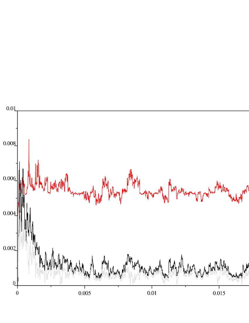
Figure 3: Field star: average cross-correlation function (middle curve), its sigma (lower grey curve) and the median ratio of the two (the upper curve) as the function of frequency ($\nu={\omega\over 2\pi}$). The LHS scale is in ${mag^{2}\over Hz}$ and relates to the bottom curves and the RHS scale relates to the ratio.

In Fig. 3 we plot $\overline{M}(\omega)$, $\sigma_{M}(\omega)$ and $\overline{M}(\omega)\over\sigma_{M}^{\prime}(\omega)$ calculated from the 12 light curves of the field star as plotted in Fig. 2. Here $\sigma_{M}^{\prime}(\omega)=\sigma_{M}(\omega)$ if $\sigma_{M}(\omega)>\langle\sigma_{M}(\omega)\rangle$ and $\sigma_{M}^{\prime}(\omega)=\langle\sigma_{M}(\omega)\rangle$ if $\sigma_{M}(\omega)\leq\langle\sigma_{M}(\omega)\rangle$. The average $\langle\overline{M}(\omega)\rangle$ = 0.00091${mag^{2}\over Hz}$ and $\langle\sigma_{M}(\omega)\rangle$ = 0.00054${mag^{2}\over Hz}$. Thus, from eq.7 we deduce $\sigma=0.023{mag\over\sqrt{Hz}}$ and eq.3 gives $\sigma=0.020{mag\over\sqrt{Hz}}$. Both numbers are consistent with each other and with average dispersion estimates from IRAF ($\sigma_{IRAF}=\sigma/\sqrt{\tau};\leavevmode\nobreak\ \tau={\it exposure\leavevmode\nobreak\ time}$). Therefore, we conclude that the test star data conform with the statistical assumptions described above.

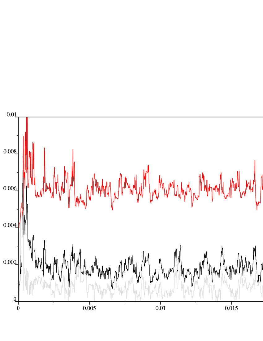
Figure 4: The average cross-correlation function, its sigma and the median ratio for pulsar data. Symbols used are the same as those in Fig. 3.

The result of a similar analysis for 16 Crab light curves is shown in Fig. 4. It is apparent that $\langle{\sigma_{M}}(\omega)\rangle$ is almost the same for the Crab and the test star; however the average $\langle\overline{M}(\omega)\rangle$ for the Crab is 1.5 times that of the test star. The process $M_{ij}(\omega)$ can, therefore, not be considered as white Gaussian noise, but it can be understood by assuming that it is the sum of a stationary “signal” $M^{0}_{ij}(\omega)$ and white Gaussian noise $M^{n}_{ij}(\omega)$ with the same spectral density as that of the test star. We considered the possibility that the “signal” is connected to a spurious phase modulation in stroboscope timing, but lab tests have set the upper limit for such a modulation some 100 times lower (Galičič c9 (1999)). We therefore conclude that the Crab pulsar light curve is intrinsically intensity modulated at the level of about 0.03$mag\over\sqrt{Hz}$. The signal to noise ratio of this modulation measure is presently too low to reveal more about its nature.

To test for the slow down of the purported free precession we recalibrate frequencies in $F_{k}(\omega)$ to the same date according to an assumed power law dependence of the free precession frequency with time, i.e. we introduce the recalibrated frequency $\tilde{\omega}=\omega({\nu_{ref}\over\nu_{k}})^{p}$, where $\nu_{ref}$ and $\nu_{k}$ are the rotation frequencies of the pulsar at the reference date (Jan.1.1996) and at the date when the k^th light curve was obtained. The above analysis has been repeated for different powers $p$ between 0 and 4. A 5.3 $\sigma$ peak stands out in $\overline{M}(\tilde{\omega})/\sigma_{M}^{\prime}(\tilde{\omega})$ and is found at $\tilde{\omega}={2\pi\over 59.93s}$ for $p$ around 1, as shown in Fig.5 and 6. Note that in the free precession model $p$ is expected to be 1 if the time for the pulsar to relax its internal stress is much longer than the total observation period ($\approx 9$years). It is expected to be 3, if this relaxation time is considerably shorter. Short relaxation times would point to externally driven precession.

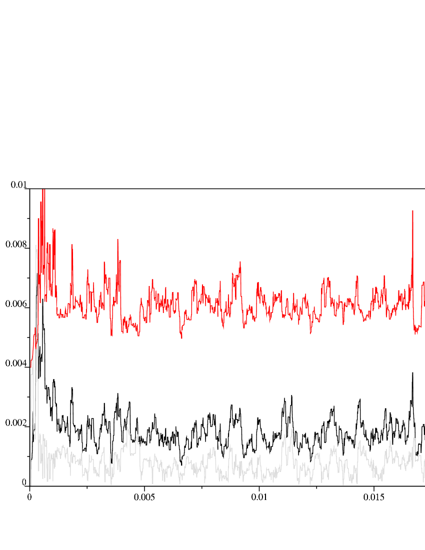
Figure 5: The average cross-correlation function ($\bar{M}(\tilde{\omega})$), its sigma ($\sigma_{M}(\tilde{\omega})$) and the median ratio $\left({{\bar{M}(\tilde{\omega})}\over{\sigma^{\prime}_{M}(\tilde{\omega})}}\right)$ for pulsar data as the function of the recalibrated frequency $\tilde{\nu}={\tilde{\omega}\over 2\pi}={\omega\over 2\pi}\left({\nu_{ref}\over\nu_{k}}\right)$, (i.e. $p=1$). Other symbols are the same as in Fig 3.

Figure 6: The peak $\overline{M}(\tilde{\omega})$ and $\overline{M}(\tilde{\omega})/\sigma^{\prime}(\tilde{\omega})$ as function of the power law index $p$

4 Discussion

The question whether pulsars free precess was raised soon after pulsars were identified as rotating neutron stars. However, more than twenty years later most astronomers would agree with Trimble and McFadden’s (c19 (1998)) somewhat humorous reference to our paper suggesting that Earth is the only known free precessing body in the Universe. We believe that pulsar free precession has evaded detection and/or identification for two main reasons. 1) Most researchers assume that neutron star matter is in a complex superfluid state, which provides an excuse to evade the question: what is the inertial eccentricity of a rotating neutron star? As a result, the range of predicted or “identified” free precession frequencies in the literature is almost without bounds, although Pines and Shaham (c16 (1974)) estimated that the Crab pulsar would wobble with a period $\simeq$ 5 minutes if it had a solid core. 2) As Alpar and Ögelman (c1 (1987)) correctly point out, free precession is a motion characteristic of rigid rotators. In a plastic rotator, free precessing motion is damped out by viscous losses - in pulsars this should happen on a time scale of years or thousands of years. Therefore, unless pulsars are exposed to reasonably large external torques, they are not expected to free precess. In our earlier paper (c7 (1997)) we tried a naive approach: starting with the observation that the Earth free precesses but taking into account the possibility that it may not be quite rigid with respect to free precession. We analysed the relation between the Earth’s inertial eccentricity, free precession frequency, rotation frequency and obliquity. We found that the Earth’s shape and that of other planets is quite similar to the equilibrium shape of rotating polytropes with no shear stress. The Earth’s free precession frequency can be fairly accurately calculated on the basis of these assumptions. We argue that a pulsar’s crust is relatively more rigid and thick than the Earth’s. Therefore, argument for planets can also be used to calculate a pulsar’s free precession frequency. For the fast Crab pulsar we found a free precession frequency on the order of $minutes^{-1}$ and in particular the theoretical value ${1\over 59.1sec}$ was found for a $1.3\,$M_⊙ pulsar model based on the tensor interaction equation of state. Surprisingly, the 35 day period of HerX-1 fits the same formula almost exactly. Our much larger dataset for the Crab pulsar strenghtens evidence for the 60 seconds period and also suggests that this period is increasing with time at almost the same rate as the rotation frequency of the pulsar. We also found that different combinations of smaller data sets consistently produce a peak at $\tilde{\omega}={2\pi\over 59.93s}$ (of course with a correspondingly smaller signal to noise ratio). In Fig. 7 we plot the Fourier amplitude of the signal in the expected frequency channel (assuming the frequency power law with $p=1$) as a function of time together with errorbars (calculated from 10 neighbouring amplitudes). Single data points are clearly very noisy, therefore, not much can be said about the time dependence - in particular the glitch of July 1996 (Jodrell Bank Crab Pulsar Monthly Ephemeris c11 ) did not leave a clear mark. The best linear fit to our data points gives an amplitude of $\Delta m(t)=(0.0045\pm 0.0006)-(0.00029\pm 0.00026)t$, where $t$ is expressed in years since 1996.0.

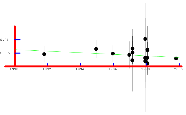
Figure 7: The spectral amplitude of the signal at the expected frequency

Does the pulsar free-precess? We presented all the evidence that we have and are inclined to believe that it does point to an affirmative answer. Open questions remain such as: 1) does the amplitude of the free precession really change with time? and 2) on what time scale does the pulsar relax its internal stress? Observation of pulsar free precession can teach us much about pulsar physics. As shown by Čadež, Galičič and Calvani c7 (1997), the free precession model can quite sensitively (if something is known about the state of internal stress) distinguish between different neutron matter equations of state. Observing the change in free precession amplitude and frequency can allow one to learn about external torques on the pulsar (jets may produce them) and also about exchange of angular momentum between the crust and the neutron superfluid. Many questions regarding the $1\over 60sec$ period remain open and, given the relevance of those questions to our understanding of pulsar physics and their interaction with neighbouring plasma, it would be important if other research groups could extend our analysis and observations.

5 Acknowledgements

We are grateful to many people who made these observations possible and who kept our sometimes dwindling spirits up. The Padua Observatory is among our staunchest supporters - in particular Massimo Calvani was supporting and stimulating our observations from the very beginning, Ulisse Munari granted us one of his nights at the 1.82m telescope and prof. Roberto Barbon was very helpful during our 1997 observations. We thank Boris Hrib for his help in the HP calibration lab and Jurij Kotar, Dick Manchester and David Nice for help with the TEMPO program. The support of the technical staff of the Guillermo Haro observatory at Cananea is kindly acknowledged. It is a pleasure also to thank Jack Sulentic for his help in making the text more readable. This program was supported in part by the Ministry of Science and Technology of the Republic of Slovenia.

References

- (1) Alpar, M. A., Ögelman, H. 1987, A&A, 185, 196
- (2) Alpar, M. A. 1989, in: Timing Neutron Stars, ed. E.P.J. van den Heuvel (Dordrecht: Kluwer Academic Publishers), 431
- (3) Carlini, A., Treves, A. 1989, AA, 215, 283-286
- (4) Čadež, A., Galičič, M. 1996a, A&A, 306, 443
- (5) Čadež, A., Galičič, M. 1996b, Is the Crab Pulsar Showing a 60-second Periodic Modulation?, in Science with the Hubble Space Telescope-II. (Benvenuti, P. ed.), Baltimore, STSCI, US Gov. Print. Office, p. 415
- (6) Čadež, A., Galičič, M. 1996c, A 60 Second Periodic Modulation in Crab Pulsar Optical Light-Curve, in Pulsars: Problems and Progress, (Johnston, S., Walker, M.A., Bailes M. eds.), ASP Conference Series, 105, 297
- (7) Čadež, A., Galičič, M., Calvani, M. 1997, A&A, 324, 1005
- (8) D’Alessandro, F., McCulloch, P. M. 1997, MNRAS, 292, 879-886
- (9) Galičič, M., 1999, Observations of Minute Time-Scales Modulation of Pulsar PSR0531+21 Optical Pulses, PhD Thesis, University of Ljubljana
- (10) Gradshteyn, I. S., Ryzhik, I. M. 1980, Table of Integrals, Series, and Products (San Diego: Academic Press)
-
(11)
Jodrell Bank Crab Pulsar Monthly Ephemeris,
http://www.jb.man.ac.uk/pulsar/crab.html - (12) Melatos, A. 2000, MNRAS, 313, 217-228
- (13) Percival, J. W. et al. 1993, ApJ, 407, 276-283
- (14) Pines, D., Shaham, J. 1974, Comm. on Mod. Phys., Part C, 6, 37
- (15) Pines, D., Shaham, J. 1973, Nat, 245, 77-81
- (16) Pines, D., Shaham, J. 1974, Nat, 248, 483-486
- (17) Shaham, J. 1977, ApJ, 214, 251-260
- (18) Shaham, J. 1986, ApJ, 310, 780-785
- (19) Trimble, V., McFadden, L. A. 1998, PASP, 110, 223-267
- (20) Ulmer, M.P. et al. 1994, ApJ, 432, 228-238