Is B1422+231 a Golden Lens?

Abstract

B1422+231 is a quadruply-imaged QSO with an exceptionally large lensing contribution from group galaxies other than main lensing galaxy. We detect diffuse X-rays from the galaxy group in archival Chandra observations; the inferred temperature is consistent with the published velocity dispersion. We then explore the range of possible mass maps that would be consistent with the observed image positions, radio fluxes, and ellipticities. Under plausible but not very restrictive assumptions about the lensing galaxy, predicted time delays involving the faint fourth image are fairly well constrained around $7h^{-1}\,\rm days$.

1 Introduction

One of the most attractive things about lensed quasars is the possibility of measuring the distance scale without any local calibrators. If the source is variable and the variation is observed in different images with time delays then a formula of the type

$$\langle\hbox{time delay}\rangle = h^{-1}z_{\rm L}(1+z_{\rm L})$$

$$\times \langle\hbox{1 month}\rangle\times\langle\hbox{image separation in arcsec}\rangle^{2}$$

$$\times \langle\hbox{lens-profile dependent factor}\rangle$$

(where $z_{\rm L}$ is the lens redshift) applies. This formula depends weakly on the source redshift (the time delay gets somewhat shorter if the source is not very much further than the lens) and on cosmology (for the same $h$ an Einstein-de Sitter cosmology gives long time delays, an open universe gives short time delays, with the currently favored flat $\Lambda$-cosmology being intermediate); but these dependencies are at the 10% level or less. The troublesome term is the lens-profile dependent factor, which is of order unity but for a given lens can be uncertain by a factor of two or more. So while the basic theory is well established (Refsdal, 1964), measuring $h$ from lensing is still problematic. Meanwhile the search for well-constrained lenses continues, and lensed-quasar aficionados speak of them as “golden lenses” (Williams and Schechter, 1997).

In this paper, we study a particularly interesting lens: B1422+231 was discovered in the JVAS survey (Patnaik et al., 1992) and consists of four images of a quasar at $z_{\rm S}\!=\!3.62$ lensed by an elliptical galaxy at $z_{\rm L}\!=\!0.334$ (Impey et al., 1996; Kochanek et al., 1998) with several nearby galaxies at the same redshift (Kundić et al., 1997; Tonry, 1998). It is especially interesting for four reasons. First, while external shear from other group galaxies is important in most four-image lenses, unlike other well-studied quads, B1422 is dominated by external shear. Second, the lensing-galaxy group can be detected directly from its X-ray emission. Third, VLBI imaging of the quasar core (Patnaik et al., 1999) gives information on not just the flux ratios but on the tensor magnification ratios. And fourth, a time delay between two images has been reported (Patnaik & Narasimha, 2001).

 

Table 1: Summary of data used for lens reconstruction (The image numbers are as shown in Fig. 1, the origin of coordinates being “G”).

image	$x$	$y$	axis ratio	PA	mag
1	$1.014$	$-0.168$	3–4	$16^{\circ}$	$15$
2	$0.291$	$0.900$	5–7	$53^{\circ}$	$30$
3	$0.680$	$0.580$	8–10	$43^{\circ}$	$-30$
4	$-0.271$	$-0.222$	1–2	$123^{\circ}$	$-1$

2 Summary of previous observations

2.1 Image configuration

Figure 1: Image configuration in B1422 (North is up, East is to the left). The filled circles labeled 1–4 mark the images, ordered by arrival time; 1 and 2 are minima, while 3 and 4 are saddle points. An unobservable fifth image would be a maximum at the center of the lensing galaxy (near ’G’). The curves are saddle-point contours in the arrival-time surface—see Blandford & Narayan (1986) for the significance of these. The precise location of the saddle-point contours in this figure are model-dependent, but the qualitative features are model-independent and generic for quads—see e.g., Figure 1 of Saha and Williams (2001).

 

The quad has three images with $V=16.5$ to $17$ nearly in a straight line, and a fourth image with $V=20$ on the other side of the galaxy (see Fig. 1). The maximum image separation is $1.3^{\prime\prime}$. Examining the image configuration and following the ideas of Blandford & Narayan (1986) on classification of images, we can work out some basic properties of the system.

First, although time delays are very uncertain, and predictions are model-dependent, the ordering of arrival times is easily inferable from the image positions and is model-independent. Thus the images can be labeled 1,2,3,4, by increasing light-travel time. Figure 1 does so. We will refer to individual images by these time-order labels.

Second, the image configuration is noticeably elongated along NE/SW. Such elongation generically indicates (Williams and Saha, 2000) that the lensing potential is significantly elongated along NW/SE. Since the main lensing galaxy is an elliptical, and cannot generate so much shear by itself, we must immediately suspect a large external shear.

2.2 External shear

Apart from qualitative evidence from the morphology, the importance of external shear in this case is further supported by the observations of galaxy group members, and a comparison with the PG1115 group. The two groups are rather similar (see Kundić et al. 1997 for comparison) including number of galaxies in the group, and the distance of the main lensing galaxy from the group’s center, about $15^{\prime\prime}$. But the apparent magnitude, and presumably the associated mass of $G$ in B1422 compared to magnitudes (and masses) of most of the other group members is small ($V_{G}=21.5$ vs. $V_{G2}=20.4$, $V_{G3}=20.0$, $V_{G4}=21.6$, $V_{G5}=20.3$), whereas in PG1115, $G$ is comparable in brightness to other group members ($R_{G}=20.2$ vs. $R_{G1}=19.0$, $R_{G2}=20.0$, $R_{G3}=20.5$). We conclude that external shear is more important in B1422 than in PG1115, and most other 4-image cases.

We can roughly estimate the magnitude of the shear. For a group or a cluster, the angular radius of the Einstein ring is

$$\theta_{\rm E}\sim 2\arcsec\times\frac{\langle\sigma_{v}^{2}\rangle}{\left(300\ {\rm km\;s}^{-1}\right)^{2}},$$

where $\sigma_{v}^{2}$ is the line-of-sight velocity dispersion of the cluster. The external shear due to this cluster (modeled as an isothermal sphere) is $\gamma\sim\theta_{E}/\theta$, where $\theta$ is the distance of the group center from the main lensing galaxy. Depending on whether $G3$ is included or excluded in the determination of the group’s velocity dispersion, $\sigma_{v}$ is $550\pm 50\,$km s^-1  or $240\pm 60\,$km s^-1. Folding in the uncertainty in the location of the group’s center, between $10^{\prime\prime}$ and $14^{\prime\prime}$, the maximum and minimum estimates of the external shear are $\gamma=0.67$ and $0.09$. Consistent with these bounds, other workers have fitted models that require $\gamma=0.25$ (Hogg & Blandford, 1994) and $\gamma\sim 0.1$ (Kormann, Schneider & Bartelmann, 1994). Using an elliptical potential model Witt & Mao (1997) derive a lower limit to the external shear of 0.11. Thus, by all accounts, the external shear plays a central role in B1422.

2.3 Magnification

The radio fluxes of the images 1,2,3 and 4 are in the ratio 16:30:33:1 at 8.4 GHz and similar at other radio frequencies (Patnaik et al., 1999; Ros et al., 2001), whereas the flux ratios in the optical and near-infrared are 8:13:16:1 (Yee & Bechtold, 1996; Lawrence et al., 1992). Reddening by the lensing galaxy is unlikely because the flux ratios do not change much between different optical wavebands. Microlensing due to stars is also unlikely because the flux ratio of images 2:3 stayed the same while both images changed in brightness (Srianand & Narasimha, private communication). This suggests that millilensing may be taking place, i.e., lensing by substructure of scale intermediate between individual stars and the whole galaxy (Mao & Schneider, 1998). If that is the case then radio fluxes are probing larger structure in the galaxy than the immediate neighborhood of the images.

Previous models, while agreeing about the direction of external shear, have been unable to to reproduce the observed flux ratios (Hogg & Blandford, 1994; Kormann, Schneider & Bartelmann, 1994; Keeton, Kochanek & Seljak, 1997; Witt & Mao, 1997).

VLBI maps by Patnaik et al. (1999) show different shapes and sizes for each image of the quasar core. It is tempting to identify the ellipticity and area of the core in each image with the relative tensor magnification; but the quoted area ratios of 1.34:1.47:1.34:1 are very different from the flux ratios, so such an identification would be incorrect. Evidently, the mapped core in image 4 corresponds to a larger area on the source than the mapped cores in images 1–3. Still, we would like to incorporate some information from these remarkable VLBI maps into our mass models. So in this paper we will adopt a compromise: we take the ellipticities of the mapped cores as the ellipticity corresponding to the magnification tensor, but we disregard the areas of the mapped cores and take the fluxes as corresponding to the scalar magnification. (How this works operationally is explained below, with equation 2.) The image and magnification data we use for modeling are collated in Table 1.

We remark that since the unlensed flux is unknown, the absolute magnifications are also unknown. This unknown factor is a manifestation of the mass disk degeneracy—see Saha (2000) and references therein.

3 Chandra X-ray observation of the group

Redshifts of six galaxies, including that of the lens, indicate that the lens is a member of a compact group whose line-of-sight velocity dispersion is 550 km/s and median projected radius $35\,h^{-1}$ kpc (Kundić et al., 1997). A Faraday rotation corresponding to a rotation measure of $280\pm 20$ rad m^-2 (Patnaik et al., 1999) between images 2 and 3 is much larger than expected from an elliptical galaxy and further supports the presence of a group around the lens.

Figure 2: Chandra ACIS-S observation of B1422+231. The X-ray observation is represented as logarithmic contours superposed on the HST H-band NICMOS image, kindly supplied by the CASTLES team. Images 2-3 and 1 are separately detected, and there is a hint of image 4 being detected as well. The pixel size of ACIS-S (0.49 arcsec) is not enough to resolve images 2 and 3. There is a slight astrometric offset between the HST and Chandra images, which we have made no attempt to correct for.

 

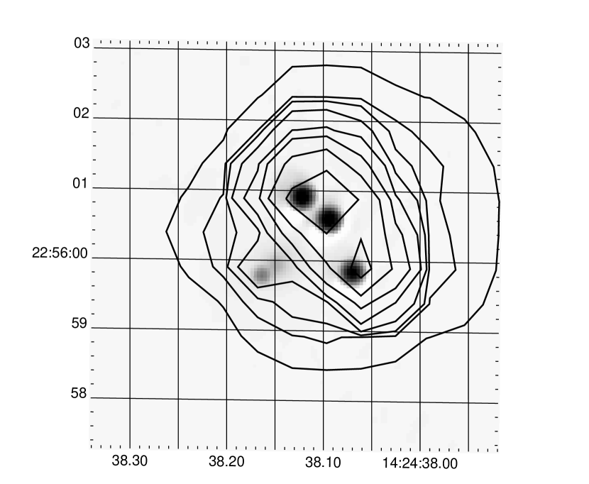
We show here the unambiguous detection of diffuse X-ray emission from hot gas belonging to this group in a Chandra observation. Previously, from a ROSAT HRI observation, Siebert and Brinkmann (1998) had found “no evidence of extended emission” over and above the $5^{\prime\prime}$ PSF of the HRI. Figure 2 shows the 28 ks Chandra ACIS-S observation represented as contours superposed on the HST image taken with the NICMOS (H-band) by the CASTLES team (Kochanek et al., 2000), where the four images, and well as the lens galaxy, are distinctly seen. There is clearly an astrometric offset between the HST and Chandra images, which we have made no attempt to correct for. However, we can safely assume that the two peaks in the X-ray distribution correspond to images 2 and 3 (brighter) and 1. The diffuse emission outside the source images is softer, and extends to a scale of about 3 arcsec, which corresponds to about $9\,h^{-1}$ kpc at the lens redshift $z=0.334$.

B1422 was observed with the ACIS-S instrument on board the Chandra observatory on 2000 June 1 for 28.8 ks, the data being collected on the back-illuminated S3 CCD. We applied the standard data processing techniques recommended by the Chandra X-Ray Center (CXC), including the recent task ACISABS, to correct for the absorption, predominantly at softer energies, caused by molecular contamination of the ACIS optical blocking filters. Since the exposure time is long enough, we reprocessed the data without randomizing the event positions, which improved the point-spread function. Periods of high background were filtered out, leaving 28.4 ks of usable data.

Figure 3: Chandra ACIS-S spectrum of B1422+231 of the diffuse emission from the lens, excluding photons from regions of radius 0.7 arcsec around each of the three QSO image regions. The best-fit model to the data in the range 0.5-6 keV (solid histogram) consists of a Raymond-Smith thermal bremsstrahlung plasma, and a power-law for the source quasar, keeping the normalization of both components free.

 

To separate the spectrum of the source quasar from that of the lensing galaxy group, we isolated circular areas of radius 0.7 arcsec around each of the three QSO images and extracted the spectrum of the quasar. The power-law fit (together with Galactic absorption) to it yielded a power-law of slope 1.41 with a reduced $\chi^{2}$ statistic of 0.9. There was no evidence of extra absorption at the redshift of the quasar. We then fixed the slope of the power law, and fitted a model of thermal bremsstrahlung plasma (Raymond-Smith) plus the quasar power-law spectrum to the rest of the X-ray emission, keeping the normalization of both components free, but fixing elemental abundance to 0.3 solar (reasonable for a group or cluster of galaxies). A fit to the data in the range 0.5-6 keV yielded a temperature of 0.71 keV for the group of galaxies, which translates into a velocity dispersion range of 150-450 km s^-1  (Helsdon & Ponman, 2000), consistent with the observed dispersion of 550, or 240km s^-1(depending on whether $G3$ is included or not). The fits were performed with the CXC software package SHERPA.

The $M-T_{X}$ relation (mass vs. x-ray temperature) for virialized isothermal systems of galaxies, for mass within a radius $0.3\,R_{\rm virial}$, gives a mass of $3.6\times 10^{12}\,M_{\odot}$ for the above temperature (Sanderson et al., 2003). The V-magnitude of the main lensing galaxy is $m_{V}=21.5$ (Kundić et al., 1997), which after correction for colour evolution (Bruzual, 2001) and $k$-correction (Frei & Gunn, 1994) yields a luminosity of $L_{B}=1.9\times 10^{10}\,h_{75}^{-2}\,L_{B,\odot}$ and a mass-to-light ratio of $M/L_{B}=190\,h_{75}$, far larger than that of a single galaxy. The bolometric X-ray flux of the diffuse emission is $L_{X}=2\times 10^{42}$ erg s^-1, which means $\log(L_{X}/L_{B})=32$, also much larger than typical values for galaxies (Helsdon et al., 2001). We therefore conclude that the diffuse emission detected by Chandra belongs to the group of galaxies the lens is a part of.

4 A simplified model

Significant external shear combined with the fortuitous positioning of the QSO source along the same line as the group and the center of the main lensing galaxy (this alignment is a robust feature in all models for this system) transforms the case of images 3 and 4 of B1422 into a one-dimensional problem. As we now show this makes the problem much better constrained than a generic 4(+1) image system.

Consider a simplified analytic model of an axisymmetric lens, with the QSO source, lens, group center, and the images all lying on the $x$-axis. Let the mass distribution in the main galaxy lens around the image-ring be given by a power law, $\rho\propto x^{-\alpha}$. Its contribution to the lensing potential is $\Phi_{\rm gal}\propto x^{2-\alpha}$, and the deflection angle is $d\Phi/dx=\pm Ax^{1-\alpha}$, where $+$ ($-$) stands for the image formed on the positive (negative) $x$-axis, and $A$ lumps together all the constants. The total lensing potential is

$$\Phi={A\over(2-\alpha)}x^{2-\alpha}+{\gamma\over 2}x^{2},$$

where we have discarded terms that are zero on the $x$-axis. The lens equation is

$$x_{I}(\gamma-1)\pm A{x_{I}}^{1-\alpha}+x_{S}=0.$$

If we define $f_{1}=x_{I}(\gamma-1)+x_{S}$ and $f_{2}=\mp A{x_{I}}^{1-\alpha}$ and plot them against lens plane coordinate $x$, then images are formed at the intersections. The four panels of Fig. 4 show models with four different combinations of ($\gamma$, $\alpha$): $(0.075,0.48)$, $(0.2,0.96)$, $(0.475,1.36)$, and $(0.725,1.9)$. All these models satisfy the locations of images 3 and 4, and the condition that image 4 arrives after 3. The vertical offset of $f_{1}$ is the source location, $x_{S}$, while external shear makes $f_{1}$ shallower. The difference in galacto-centric distances of images 3 and 4 is given by $|x_{3}+x_{4}|$.

Figure 4: B1422 simplified: one dimensional case showing the formation of images 3 and 4. Thick dashed lines represent $f_{1}=x_{I}(\gamma-1)+x_{S}$ and thick solid lines represent $f_{2}=\mp A{x_{I}}^{1-\alpha}$; they intersect at image locations. Four combinations of ($\gamma$, $\alpha$) are shown in the four panels, as labeled. The thin dotted lines show the axes, the diagonals, and image locations.

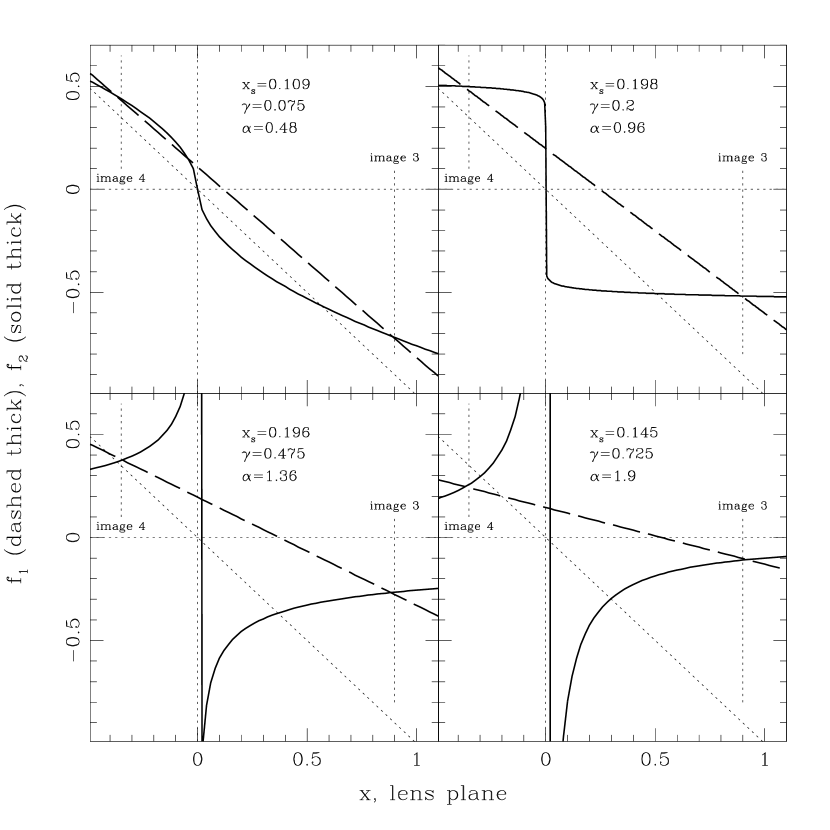
Figure 4 graphically demonstrates that in a system where images are formed at very different galacto-centric distances (like 3 and 4 in B1422) there is a limit to the shallowness of the galaxy’s density profile index, $\alpha$. It is clear from the figure that some non-zero $x_{S}$ is needed to produce large $|x_{3}+x_{4}|$. For shallow density profiles (such as the one in the upper left panel) $f_{2}$ tends to become the diagonal through the II and IV quadrant. This makes it very difficult to have $f_{2}$ intersect $f_{1}$ while keeping $|x_{3}+x_{4}|$ large. The lower limit on $\alpha$ is around $\sim 0.5$.

The figure also shows that $\alpha$ and $\gamma$ in B1422 are correlated: as profile slopes get steeper, shear must increase as well. For $\alpha>1$ (profile steeper than isothermal) $f_{2}$ become hyperbolic, and a substantial flattening of $f_{1}$ (i.e. large external shear) is required to produce large $|x_{3}+x_{4}|$. Note that large shear is necessary for this; a large $x_{S}$ by itself is not sufficient.

As long as profile is steeper than a minimum $\alpha$ value, one-dimensional lensing case does not prefer large $\gamma$, large $\alpha$ solutions over small $\gamma$, small $\alpha$: in Fig. 4 $(\gamma,\alpha)=(0.075,0.48)$ is as good a fit as $(0.725,1.9)$. However, when we consider two dimensions, images 1 and 2, set an upper limit on the external shear because too large a shear will tend to place images 1, 2 and 3 in a straight line, perpendicular to the direction towards external shear. Since observed images 1,2 and 3 are not in a straight line, the shear is constrained from above. Furthermore, if the tensor magnification information is included in modeling (as is done in Section 5) the relative orientation of these for images 1 and 2 also reduced the amplitude of possible shear.

We can intuitively understand the effect of external shear on the time delays $\Delta t$ as follows. If the shear source is far from the image region, the shear can be represented by constant external shear, which provides linear deflection angles at the images. It corresponds to tilting the side of the arrival-time surface closest to the source of the shear upwards, which moves the zero points in $\Delta t$ away from the shear source. Images lying on the line through the shear source, QSO source and the main galaxy are most affected by this tilting (images 3 and 4 in B1422), while those lying perpendicular to that line are least affected (1 and 2). Thus images 3 and 4 give a well constrained $\Delta t$, precisely because they are most sensitive to external shear.

To sum up, the fortuitous geometry of B1422 and large external shear imply a relation between profile slope and shear magnitude, and impose a limit on the shallowness of the profile slope of $\alpha\sim 0.5$, or a lower limit on shear of $\gamma\sim 0.1$, consistent with the shear estimates based on the physical properties of the group (Section 2.2). In addition, images 1 and 2 impose a limit on the steepness of the profile slope (through an upper limit on shear). As a result, $\Delta t_{34}$ should be well constrained.

5 Pixelated models

We now consider more detailed models of galaxy mass distribution in the lens plane.

Given the difficulties caused to previous models of B1422 by the observed flux ratios, and especially since we now need to fit tensor magnifications, it is clear that more general models than those are necessary. Moreover, to properly estimate uncertainties, it is necessary to explore not just a few models but large ensembles of them. The pixelated lens reconstruction method, as developed in Saha & Williams (1997) and Williams and Saha (2000), was designed for this purpose. The idea is to model the lens as a sum of mass tiles or pixels, with two kinds of constraints: the “primary constraints” are that the lensing data should be fitted exactly; “secondary constraints” require the mass distribution to be centrally concentrated, not excessively elongated, and optionally inversion-symmetric. Here we follow the method of generating ensembles of models as detailed in the latter paper, but with two minor modifications necessitated by the type of data.

The first modification is needed because the time delay measurements are currently very uncertain. So instead of including them, we run the reconstruction code with one time delay ($\Delta t_{34}$, say) set to a fiducial value $d_{\rm fid}$. The code then generates an ensemble of models, each model having its own $h$ and its own set of $\Delta t_{ij}$. Because of the scaling properties of the lensing problem, the only dependence of the results on $d_{\rm fid}$ will be that all the model $h^{-1}$ and $\Delta t_{ij}$ will be proportional to it. Hence $h\Delta t_{ij}$ will be independent of $d_{\rm fid}$.

A second modification is needed to incorporate tensor magnifications. To do this, we first reconstruct the magnification matrix M at each image position from the data in Table 1. We have

$${\bf M}={\bf R}(-\omega)\pmatrix{\sqrt{Mr}&0\cr 0&\sqrt{M/r}}{\bf R}(\omega)$$ (2)

where $M$ is the scalar magnification (proportional to the flux), $r$ is the axis ratio (if we assume the source is circular), $\omega$ is the orientation ($\rm PA+90^{\circ}$), and R is a rotation matrix. The signs of the square roots in equation 2 depend on image parity: for minima both roots will be positive; for saddle points one will be negative. Having reconstructed M at the image positions, we write the observed upper and lower bounds on the axis ratio as bounds on the ratio of the diagonal elements of M (see AbdelSalam et al. (1998) for an application of this technique to arclets in cluster lensing). Having constrained the axis ratio, we set the flux ratio by introducing a fictitious quad slightly displaced from the actual one; in particular, fictitious images displaced by

$$\pmatrix{\Delta\theta_{x}\cr\Delta\theta_{y}}={\bf M}\pmatrix{\epsilon\cr 0}$$ (3)

correspond to a fictitious source displaced by $\epsilon$ along the $x$-axis of the source plane. The code is not told $\epsilon$ itself, just the displacements it maps to; in this way the magnification ratios are constrained, but not the absolute magnifications.

We have generated three ensembles of models. Each ensemble contains 100 models sampling the allowed ‘model space’ given a certain set of constraints.

Figure 5: Ensemble average of 100 mass maps including tensor magnification and assuming inversion symmetry. The pixel size is evident. Contours are in steps of $1\over 3$ of the critical density for lensing, with the outermost contour at $1\over 3$ of the critical density. The filled circles indicate the image, and dashed ellipses around them indicate the tensor magnification. But note that we have made the areas of the ellipses proportional to $\sqrt{M}$ rather than $M$.

Figure 6: Left panel: Predicted time delays (in the form $h\Delta t$ in days) between images 3 and 4, for the same ensemble as in Fig. 6. Other panels: Predicted time delays between different images (going downwards, 1–2, 2–3, and 3–4) for the same ensemble. Note that the horizontal scale varies between panels.

The first ensemble uses the data from Table 1, together with the generic secondary constraints (Williams and Saha, 2000) including inversion symmetry of galaxy-lens. Figure 6 shows the ensemble-average mass map, while Fig. 6 shows the distribution of predicted time delays. (The ‘radial profile index’ in Fig. 6 corresponds approximately to $-\alpha$ in the previous section.) The qualitative results are just as expected from our preceding discussion: (i) images 1,2,3 are very close in $\Delta t$, with 4 arriving much later; (ii) $\alpha$ is nearly confined to a narrow range 0.6–0.8; (iii) while $\Delta t_{34}$ has a broad peak with median $7.3h$ days, it is much better constrained than in models of other well-studied quads (Williams and Saha, 2000).

For the second ensemble we dropped the inversion-symmetry constraint. Figures 8 and 8 show the results. Qualitatively, the results are similar, but the predicted $\Delta t_{34}$ shifts to a higher range (median $12.4h$ days). One must keep in mind that observed image properties tightly constrain the position angle of the shear, not its radial location. So non-inversion-symmetric modeling of lens systems with large external shear will produce mass profiles that are artificially elongated towards the source of external shear. This is seen in Fig. 8. The elongation results because the model cannot decide how far away to place the source of the shear. Thus, for systems with non-disturbed galaxy lenses and large external shear the inversion-symmetric models are probably somewhat more trustworthy than non-inversion-symmetric ones.

Figure 7: Like Fig. 6, but without the inversion-symmetry constraint.

Figure 8: Like Fig. 6, but for models without the inversion symmetry constraint.

For the third ensemble we put back the inversion-symmetry constraint, but drop the magnification constraint. Figure 9 shows the time-delay predictions. (The ensemble-average mass map looks similar to Fig. 6 and we have not included it here.) Comparison of Fig. 9 and Fig. 6 shows what magnification information adds to modeling. Basically, magnification measurements put constraints on the mass distribution in the neighborhood of the images. Time delays between nearby images becomes better constrained. Thus Fig. 9 has a much larger spread in $\Delta t_{12}$ and $\Delta t_{23}$ than Fig. 6. Without magnifications, some models’ $\Delta t_{12}$ or $\Delta t_{23}$ can become zero: magnifications for the images in question can get arbitrarily large, effectively merging those images. Also, the upper bound on $\alpha$ that we argue comes from images 1 and 2 is greatly weakened. On the other hand, time delays between distant images is hardly affected: as anticipated in Section 4, $\Delta t_{34}$ in Fig. 9 has a median ($7.8h$ days) and range very similar to those in Fig. 6.

Figure 9: Like Fig. 6, but for models without magnification constraints.

 

6 Conclusions

In the Introduction, we mentioned four unusual features that make B1422 a particularly interesting lens. We now summarize what the results of this paper indicate about each of these features.

First, we have the surprising result that being dominated by external shear from group galaxies makes the lens better constrained. The predicted time delays, in particular the longest delay $\Delta t_{34}$, though it has a broad range, is narrower than in other comparable systems. The fortuitous alignment of the source displacement and the shear appears to help.

Second, one detail of the group contribution is important. Of two situations: (i) the lensing galaxy has $180^{\circ}$-rotation symmetry and the shear comes from relatively distant group members, and (ii) the lensing galaxy is asymmetric and elongated along the group direction, the second case gives $\Delta t_{34}$ 50% longer. Optical and X-ray (see Fig. 2) images of the galaxy and group are not conclusive on this point.

Third, tensor magnifications from fluxes and VLBI constrain time delays between nearby images; but remarkably they have no discernible effect on longer time delays, $\Delta t_{34}$. The physical reason is not hard to appreciate: magnification is essentially the second derivative of the time delay, hence time delays between widely separated images tend to wash out the sort of local variations of density that cause differences in magnifications.

Fourth, comparison with time-delay measurements is still problematic at present. Patnaik & Narasimha (2001) report $\Delta t_{12}=7.6\pm 2.5\rm d$, whereas our reconstructions predict $\Delta t_{12}\sim 0.4h\rm d$. The difficulty is that our predicted values would not be expected to show up in the Patnaik & Narasimha data, which sample at $\sim 4\rm d$; instead, aliases of our predicted values would show up. Even with closely-sampled data, a $\Delta t_{12}\sim 0.4h\rm d$ is unlikely to be measurable because it would need intrinsic brightness variations on the scale of hours. On the other hand, the predicted $\Delta t_{34}\sim 5-10\rm d$ is a convenient length for measurements; but unfortunately it involves image 4, whose flux is $\sim 30$ times smaller.

In summary, we conclude that B1422 is a very interesting lens, but probably not the sought-after golden lens.

References

- AbdelSalam et al. (1998) AbdelSalam, H. M., Saha, P., & Williams, L. L. R., 1998, AJ, 116, 1541
- Blandford & Kundić (1996) Blandford, R.D. & Kundić, T. 1996, Conf. Proc., The Extragalactic Distance Scale, Cambridge Univ. Press, ed. M. Livio, p. 60
- Blandford & Narayan (1986) Blandford, R. D. & Narayan, R. 1986, ApJ, 310, 568
- Bruzual (2001) Bruzual A., G. 2001, Astrophysics and Space Science Supplement, 277, 221 (astro-ph/0011094)
- Chang & Refsdal (1979) Chang, K. & Refsdal, S. 1979, Nature, 282, 561
- Frei & Gunn (1994) Frei, Z. & Gunn, J. E. 1994, AJ, 108, 1476
- Helsdon & Ponman (2000) Helsdon, S. F., Ponman, T. J. 2000, MNRAS, 319, 933
- Helsdon et al. (2001) Helsdon, S. F., Ponman, T. J., O’Sullivan E. & Forbes D. A. 2001, MNRAS, 325, 693
- Hogg & Blandford (1994) Hogg, D. W. & Blandford, R. D. 1994, MNRAS, 268, 889
- Impey et al. (1996) Impey, C. D., Foltz, C. B., Petry, C. E., Browne, I. W. A. & Patnaik, A. R. 1996, ApJ, 462, L53
- Keeton, Kochanek & Seljak (1997) Keeton, C. R., Kochanek, C. S. & Seljak, U. 1997, ApJ, 482, 604
- Kochanek et al. (2000) Kochanek, C. S. et al. 2000, ApJ, 543, 131
- Kochanek et al. (1998) Kochanek C. S., Falco E. E., Impey C., Lehar J., McLeod B., & Rix H.-W. 1998, http://cfa-www.harvard.edu/castles/
- Kormann, Schneider & Bartelmann (1994) Kormann, R., Schneider, P. & Bartelmann, M. 1994, A&A, 286, 357
- Kovner (1987) Kovner, I. 1987, ApJ, 318, L1
- Kundić et al. (1997) Kundić, T., Hogg, D. W., Blandford, R. D., Cohen, J. G., Lubin, L. M. & Larkin, J. E. 1997, AJ, 114, 2276
- Lawrence et al. (1992) Lawrence, C. R., Neugebauer, G., Weir, N., Matthews, K. & Patnaik, A. R. 1992, MNRAS, 259, 5P
- Mao & Schneider (1998) Mao, S. & Schneider, P. 1998, MNRAS, 295, 587
- Patnaik et al. (1999) Patnaik, A. R., Kemball, A. J., Porcas, R. W. & Garrett, M. A. 1999, MNRAS, 307, L1
- Patnaik & Narasimha (2001) Patnaik, A. R. & Narasimha, D. 2001, MNRAS, 326, 1403
- Patnaik et al. (1992) Patnaik, A. R., Browne, I. W. A., Walsh, D., Chaffee, F. H. & Foltz, C. B. 1992, MNRAS, 259, 1P
- Refsdal (1964) Refsdal, S. 1964, MNRAS, 128, 307
- Ros et al. (2001) Ros, E., Guirado, J. C., Marcaide, J. M., Pérez-Torres, M. A., Falco, E. E., Muñoz, J. A., Alberdi, A., & Lara, L. 2001, Highlights of Spanish astrophysics II, 49
- Saha (2000) Saha, P., AJ, 120, 1654
- Saha & Williams (1997) Saha, P., & Williams, L. L. R. 1997, MNRAS, 292, 148
- Saha and Williams (2001) Saha, P., & Williams, L. L. R. 2001, AJ, 122, 585
- Sanderson et al. (2003) Sanderson, A., Ponman, T.J., Finoguenov, A., Lloyd-Davies, E. & Markevitch, M., 2003, MNRAS, in press
- Siebert and Brinkmann (1998) Siebert & Brinkmann 1998, A&A, 333, 63
- Tonry (1998) Tonry, J. L. 1998, AJ, 115, 1
- Williams and Saha (2000) Williams, L. L. R. & Saha, P. 2000, AJ, 119, 439
- Williams and Schechter (1997) Williams, L. L. R. & Schechter, P. L., 1997, Astronomy & Geophysics, 38, 10
- Witt & Mao (1997) Witt, H. J., Mao, S. 1997, MNRAS, 291, 211
- Witt, Mao & Keeton (2000) Witt, H. J., Mao, S. & Keeton, C. R. 2000, ApJ, 544, 98
- Yee & Bechtold (1996) Yee, H. K. C. & Bechtold, J. 1996, AJ, 111, 1007