The VLA-VIRMOS Deep Field

We have conducted a deep survey (r.m.s noise $\simeq 17\mu$Jy) with the Very Large Array (VLA) at 1.4 GHz, with a resolution of 6 arcsec, of a 1 deg² region included in the VIRMOS VLT Deep Survey. In the same field we already have multiband photometry down to $I_{\rm AB}=25$, and spectroscopic observations will be obtained during the VIRMOS VLT survey. The homogeneous sensitivity over the whole field has allowed to derive a complete sample of 1054 radio sources ($5\sigma$ limit). We give a detailed description of the data reduction and of the analysis of the radio observations, with particular care to the effects of clean bias and bandwidth smearing, and of the methods used to obtain the catalogue of radio sources. To estimate the effect of the resolution bias on our observations we have modelled the effective angular-size distribution of the sources in our sample and we have used this distribution to simulate a sample of radio sources. Finally we present the radio count distribution down to 0.08 mJy derived from the catalogue. Our counts are in good agreement with the best fit derived from earlier surveys, and are about 50% higher than the counts in the HDF. The radio count distribution clearly shows, with extremely good statistics, the change in the slope for the sub-mJy radio sources.

1 Introduction

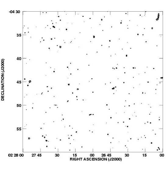
Figure 1: South-eastern quadrant of the VLA-VDF radio image. Contours are in units of signal to noise ratio, first contour is $5\sigma$.

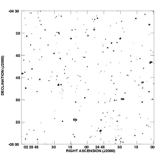
Figure 2: South-western quadrant of the VLA-VDF radio image. Contours are in units of signal to noise ratio, first contour is $5\sigma$.

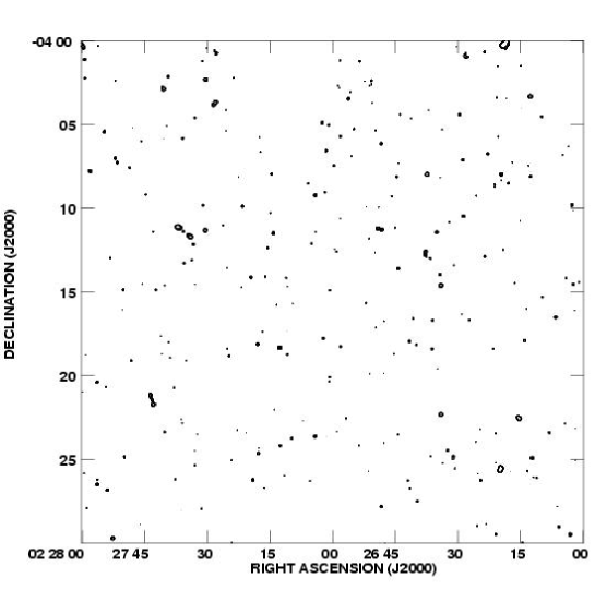
Figure 3: North-eastern quadrant of the VLA-VDF radio image. Contours are in units of signal to noise ratio, first contour is $5\sigma$.

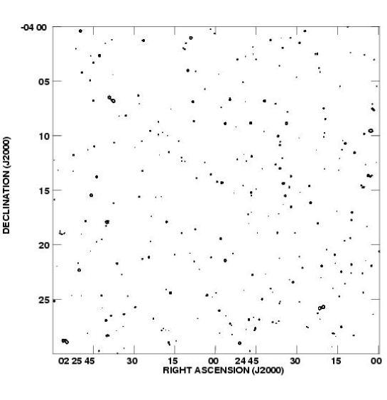
Figure 4: North-western quadrant of the VLA-VDF radio image. Contours are in units of signal to noise ratio, first contour is $5\sigma$.

It is well established that the 1.4 GHz source counts at sub-mJy levels reveal the presence of a population of faint radio sources far in excess with respect to those expected from the high luminosity radio galaxies and quasars which dominate at higher fluxes (Windhorst et al. (1985); Condon (1989); Hopkins et al. (1998);  Ciliegi et al. (1999); Richards (2000); Prandoni et al. 2001a ;  Gruppioni et al. 1999b ). Early spectroscopic studies, limited to relatively bright optical counterparts (B$\leq$21.5-22.0; Benn et al. (1993)), suggested that most of these sub-mJy radio sources were starburst galaxies. However it has been shown that the predominance of starburst galaxies is dependent on the magnitude limit of the spectroscopic follow up (Gruppioni et al. 1999a ; Prandoni et al. 2001b ). While at bright magnitude (B${{}_{<}\atop{}^{\sim}}22$) most of the optical counterparts are indeed starburst galaxies, at fainter magnitudes (B${{}_{>}\atop{}^{\sim}}22.5$) most of the optical counterparts appear to be early type galaxies. This mixture of at least two different populations is consistent with what is being found at even fainter radio fluxes, in the $\mu$Jy regime, where high-$z$ early type galaxies, intermediate-$z$ post starburst galaxies, and lower-$z$ emission line galaxies are found in approximately similar proportions (Hammer et al. (1995); Windhorst et al. (1995); Richards et al. (1998)).

In order to fully investigate the nature and evolution of the sub-mJy population it is absolutely necessary to couple deep radio and optical (both imaging and spectroscopic) observations over a reasonably large area of the sky.

The VIRMOS VLT Deep Survey (VVDS, Le Fevre et al. (2002)) will produce spectroscopic redshifts for about $1.5\times 10^{5}$ galaxies in an area of $\sim 16$ deg² selected from an unbiased photometric sample of more than 1 million galaxies. We have selected a 1 deg² field from the VVDS, centered at RA(J2000)=02:26:00 DEC(J2000)=$-04$:30:00, for deep VLA radio observations at 1.4 GHz (hereafter the VLA-VIRMOS Deep Field, VLA-VDF). This field is ideal for a radio survey as UBVRI photometry, complemented by K band data on a smaller region, is already available to $I_{\rm AB}\simeq 25$ (Le Fevre et al. (2001)), and spectroscopy is being obtained to $I_{\rm AB}=24-24.5$ with the VIMOS spectrograph at the VLT (Le Fevre et al. (2001)).

In this paper we present the VLA radio observations at 1.4 GHz of the VLA-VIRMOS Deep Field, discuss the methods used to derive the catologue of about 1000 radio sources (down to a limit of 80 $\mu$Jy) and derive the radio source counts. The identification of the radio sources using the multi-band photometry will be discussed in a following paper (Ciliegi et al. (2002)). In Sect. 2 the observations and data reduction are presented. Sect. 3 contains a detailed description of the analysis carried out on the radio mosaic in order to quantify the effects of clean bias and bandwidth smearing on our observations. The procedure adopted to obtain a complete catalogue of radio sources from the radio mosaic is presented in Sect. 4. Finally, in Sect. 5 we derive the radio counts corrected for the resolution bias. Conclusions are given in Sect. 6.

2 The VLA Observations

The observations were obtained at the Very Large Array (VLA) in B-configuration for a total time of 56 hours over 9 days from November 1999 to January 2000. This configuration was adopted as the best choice in order to obtain a deep survey of a relatively large (1 square degree) area of the sky with an acceptable resolution.

At 1.4 GHz the VLA antennas have a primary beam with a FWHM of 31 arcmin. In order to image with uniform sensitivity a 1 square degree field it is necessary to make multiple pointings displaced by about $31/\sqrt{2}\sim 22$ arcmin (Condon et al. (1998); Becker et al. (1995)). We chose to cover the surveyed area with a square grid of 9 pointings, separated by 23 arcmin in right ascension and declination. Such a geometry allows to reach theoretical noise variations smaller than $10\%$ over $95\%$ of the 1 deg² field. Each of the pointing centers was observed for a total of about 6 hours, including the observations of the calibrators. Every 20 minutes we interleaved the scans on the nine pointings with a short observation of the source J0241$-$082 to provide amplitude, phase, and bandpass calibration.

The observations were carried out in bandwidth synthesis mode to avoid substantial chromatic aberration (bandwidth smearing). In this way it is also possible to reduce the effects of narrow-band interferences since only the channel affected by the interferences, instead of the whole bandwidth, can be removed from the data. The data were collected in spectral line mode using two intermediate frequency (IF) bands centered at 1364.9 MHz and 1435.1 MHz. Each IF was divided in 7 channels each 3 MHz wide. Due to limitations in the VLA correlator only circular polarization modes were recorded.

2.1 Calibration & Editing

The data were reduced and analyzed using the package AIPS developed by the National Radio Astronomy Observatory. The amplitude calibration was derived from daily observations of 3C 48 assuming flux densities of 16.51 Jy at 1365 MHz and 15.87 Jy at 1435 MHz. The AIPS tasks UVLIN and CLIP were used to flag bad visibility data resulting from radio frequency interferences, receiver problems or correlator failures. The task UVLIN was run after the amplitude calibration with a threshold of 1 Jy. After UVLIN, the task CLIP was run on a channel-by-channel basis with a threshold determined by the task UVPRM (8 times the rms of the data). The task UVFIX was run to improve the astrometric solution and then the data sets for each pointing were combined and inspected for further editing.

2.2 Imaging, self calibration and mosaicing

Self calibration and imaging of wide field deep observations is a time consuming task. For each pointing we imaged a $2048\times 2048$ pixels area ($51\times 51$ arcminutes, 1 pixel corresponds to 1.5 arcsec) along with a number of smaller images (usually $32\times 32$ pixels) centered on off-axis sources that can produce confusing grating rings in the imaged area. The possibly confusing sources have been identified with the RUN file generator applet available at the NVSS home page, selecting all the sources with peak flux density greater than 1 mJy (at the NVSS resolution) within a radius of 60 arcmin of each pointing and not included in the main field area.

To avoid distorsions due to the use of two dimensional FFT to approximate the curved celestial sphere, the $2048\times 2048$ pixels area of each pointing was not deconvolved as a single image but was split in a number of sub-images (e.g. Perley (1999)). At the end of the self-calibration deconvolution iteration scheme, the sub-images were combined together using the AIPS task PASTE to produce the final $2048\times 2048$ pixels image of each single pointing. The final images have been restored with a $6\times 6$ arcseconds FWHM gaussian beam. We self-calibrated and cleaned the different pointings in a way as homogeneous as possible in order to minimize differences in the sensitivity. Clearly, the presence or absence of relatively strong ($\simeq 10$ mJy/beam) sources in some fields and the fluctuations in the noise produced slightly different noise figures, with 1 $\sigma$ rms noise ranging from 14.8 to 17.9 $\mu$Jy/beam, in the nine pointings. Finally, the 9 pointings have been combined together using the task HGEOM and LTESS obtaining a linear combination weighted by the square of the beam response. The average noise over the full 1 square degree field in the mosaic map is 17.5 $\mu$Jy. In Fig. 1-4 we show the final image of the 1 square degree VLA-VIRMOS deep field split in four quadrants for a clearer representation. The noise over the 1 square degree field is homogeneous (see also Sect. 4.1) and the few regions devoid of sources visible in Fig. 1-4 (the most notable of which is the area around right ascension 02:25:40 and declination -04:52:00) are real and not artifacts produced by a much higher local noise.

3 Analysis

3.1 Clean bias

Clean bias is a recently recognized possible source of error in the flux density estimate derived from interferometer snapshot observations. The FIRST and NVSS VLA surveys, for example, are affected by this bias and the flux densities derived from the publicly available images have to be corrected a-posteriori. The effect of the clean bias is that flux densities of real sources are sistematically underestimated because the CLEANing algorithm subtracts flux from real sources and redistributes it on top of noise peaks or sidelobes. This effect is dependent on the image noise and synthesized beam sidelobe levels and mostly independent from the source flux density (Becker et al. (1995); Condon et al. (1998)).

The VLA-VDF observations are very long compared to the snapshots of the VLA surveys, and consequently the synthesized beam has much lower sidelobes. For instance, the NVSS observations have a synthesized beam with sidelobes reaching about $25\%$ of the main lobe, while the sidelobes in the synthesized beam of the VLA-VDF observations reach only $1.6\%$ of the main lobe. A good rule of thumb to avoid clean bias is to minimize the clean area and not to clean the image down to the theoretical noise. The first prescription is hard to follow as our goal is to image a 1 square degree field. On the other hand, we used a rather conservative approach halting the clean process when the clean residuals were between 2 and 5 times the theoretical r.m.s. noise. While we can expect that the clean bias in our observations is much lower than that affecting snapshot observations, we can not rule it out completely a-priori. In order to assess the impact of the clean bias on the VLA-VDF observations we have used two different methods.

The first method is a step-by-step clean. We can expect that beyond a threshold value in the number of iterations, the clean bias begins to be important and the flux density of the components in these maps becomes sistematically lower than that of the corresponding components in the images with less iterations. About $4\times 10^{4}$ clean iterations are the minimum number necessary to effectively approach the expected noise for the $2048\times 2048$ pixel images. We have then chosen one of the nine fields and produced different images with an increasing number of clean iterations. We have produced images with $4\times 10^{4}$, $5\times 10^{4}$, $7.5\times 10^{4}$ and $5\times 10^{5}$ iterations and on each of them we have identified radio components down to the $3\sigma$ limit. For each component we have extracted the peak flux and computed the difference of fluxes obtained between maps with different iteration limits. The median of these differences is listed in Table 1.

Table 1: Clean bias simulation

Niter(1)$-$Niter(2)	median $\Delta S$
$40000-50000$	0.5 $\mu$Jy/beam
$50000-75000$	1.0 $\mu$Jy/beam
$75000-500000$	14.4 $\mu$Jy/beam

As can be seen from Table 1, increasing the number of iterations to $5\times 10^{4}$ or even $7.5\times 10^{4}$ produces a systematic decrease in the peak flux densities of about 1.0 $\mu$Jy/beam or less. We have to push the clean to a far higher number of iterations to start seeing a significant effect due to the clean bias. Using $5\times 10^{5}$ iterations we find a decrease in the peak flux density of the sources with a median of 14.4 $\mu$Jy/beam. We have then chosen a limit of about $5\times 10^{4}$ clean iterations for each of the nine fields. This means that any clean bias affecting our brightness measurements should be less than 1 $\mu$Jy/beam and then practically negligible.

The second method used to verify the absence of a significant effect produced by the clean bias was to insert artificial sources with known flux in the uv-data set of a chosen field. In particular, we have modified the uv-data set of a randomly chosen field adding 25 point sources with 0.5 mJy flux. We have then cleaned the field to the same depth used for the original one and compared the fluxes of the artificial sources on the map with their true fluxes. We have repeated this operation four times obtaining a set of 100 artificial sources at different positions. The mean of the peak flux density distribution of these 100 sources is $0.503\pm 0.003$ mJy/beam. We can conclude that both methods confirm that the flux density derived from our images are not affected by the clean bias.

3.2 Bandwidth Smearing

Imaging sources at large distances from the phase center can result in radial smearing reducing the peak flux density of a source while conserving its integrated flux density. This effect is known as bandwith smearing (or chromatic aberration) and affects all the synthesis observations made with a finite bandwidth. The image smearing is proportional to the bandwidth and to the distance of the source from the phase center. In order to image a 1 square degree field we have to minimize the effect of bandwith smearing and for this reason we observed in spectral line mode. Nonetheless, some amount of smearing can still be present in our images. To check this effect on our observations we have observed the radio source 3C84 at different position offsets (0, 5, 10, 20, 30 arcmin) in two orthogonal directions. The images of 3C84 at different offsets have been fitted with a two dimensional gaussian to derive the peak and integrated flux density. The mean ratio between these two quantities is shown in Fig. 5. At the distance between the pointing centers (23 arcmin) $S_{\rm P}/S_{\rm T}\sim 0.96$. Since the nine radio fields are combined together weighted by the square of the beam response, we can conclude that the effect of the bandwidth smearing is negligible.

Figure 5: Ratio between $S_{\rm P}$ and $S_{\rm T}$ for 3C 84 as a function of off-axis angular distance as a test of bandwidth smearing for the VLA-VDF observations. The vertical line indicates the distance between adjacent pointing centers.

4 From the radio mosaic to the catalogue

4.1 The noise map

Having verified that clean bias and radial smearing do not significantly affect the determination of the flux densities in the VLA-VDF, we started to work on the extraction of a catalogue from the mosaic image. In order to select a sample above a given threshold, defined in terms of local signal to noise ratio, we performed a detailed analysis of the spatial root mean square (rms) noise distribution over the entire mosaic image using the software package SExtractor (Bertin & Arnouts (1996)). To construct the noise map, SExtractor makes a first pass through the pixel data, computing an estimator for the local background in each mesh of a grid that covers the whole frame (see Bertin & Arnouts (1996) for more details). The choice of the mesh size is very important. When it is too small, the background estimation is affected by the presence of real sources. When it is too large, it cannot reproduce the small scale variations of the background. For our radio mosaic we adopted a mesh size of 20 pixels, corresponding to 30 arcsec. A grey scale of the noise map obtained with SExtractor is shown in Fig. 6, while Fig. 7 shows the histogram of its pixel values. Due to the uniform noise over the whole field the pattern of the 9 pointings used for our observations can be barely seen in Fig. 6. The areas of higher noise (black pixels) are due to the presence of relatively strong radio sources (10-20 mJy/beam) in the map. The pixel values distribution has a peak at 16 $\mu$Jy/beam, well in agreement with the noise values found in Sect. 3.2.

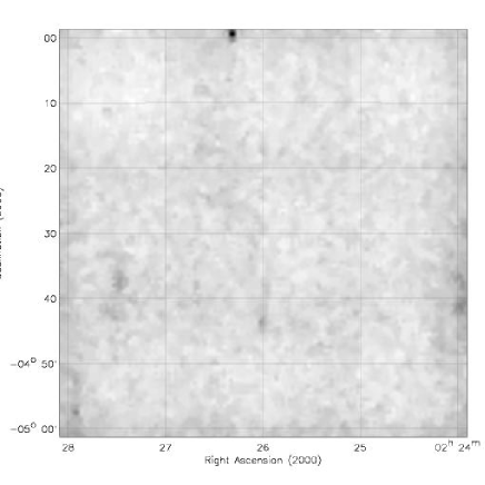
Figure 6: A grey scale of the noise map (1 $\times$ 1 deg²) obtained with SExtractor. Darker regions mean higher noise.

Figure 7: Distribution of the pixel values of the noise map obtained with SExtractor

Since SExtractor was developed for the analysis of optical data and this is the first attempt in using it on a radio map, we tested the reliability of its output by constructing a noise map with a completely independent software written in IDL language. Briefly, starting from the residual map obtained from the AIPS task SAD where all the sources with peak flux greater than 60 $\mu$Jy ($\sim 3.5\sigma$) have been subtracted, we have first removed the most anomalous residual pixels (including extended sources not found or rejected by SAD) substituting these values with the average rms obtained from the residual map. Then, we applied a local sigma clipping, substituting all the pixel values greater than 3 times the local sigma with a random value extracted from a Gaussian with mean and sigma equal to the local values. Finally, the noise map has been obtained substituting each pixel value with the standard deviation values calculated in a local box around each pixel (we used a box of 20$\times$20 pixels). In Fig. 8 we show the distribution of the ratio (pixel by pixel) between the noise map obtained with SExtractor and that obtained with our IDL code. A detailed analysis of the two maps shows that they are in very good agreement with each other, with differences of pixel values which are smaller than $25\%$ over about $96\%$ per cent of the area.

Figure 8: Distribution of pixel by pixel ratio between the noise map obtained with SExtractor and the noise map obtained with our IDL code

On the basis of this comparison we concluded that the noise map obtained with SExtractor is indeed reliable and we used it for the extraction of a catalogue.

4.2 The source detections

The area from which we have extracted the complete sample of sources is 1$\times$1 deg² centered at RA=02:26:00 DEC=$-04$:30:00 (J2000). Within this region we extracted all the radio components with a peak flux S${}_{\rm P}>$60 $\mu$Jy ($\sim 3.5\sigma$) using the AIPS task SAD (Search And Destroy), which attempts to find all the components whose peaks are brighter than a given level. For each selected component, the peak and total fluxes, the position and the size are estimated using a Gaussian fit. However, for faint components the Gaussian fit may be unreliable and a better estimate of the peak flux S_P (used for the selection) and of the component position is obtained with a simple interpolation of the peak values around the fitted position. Therefore, starting from the SAD positions, we derived the peak flux S_P and the position of all the components using a second-degree interpolation with task MAXFIT. Only the components for which the ratio between the MAXFIT peak flux density and the local noise (derived from the noise map described in the previous section) was greater or equal to 5 have been included in the sample. A total of 1084 components have been selected with this procedure.

Some of these components clearly belong to a single radio source (e.g. the lobes of a few FR II radio sources, or components in very extended sources), but for most of them it is necessary to derive a criterion as general as possible to discriminate between different components of the same radio source or truly different radio sources. For this reason, the components with distance less than 18 arcseconds (3 times the beam size) have been selected as possible doubles and have been visually checked one-by one using also preliminary deep optical images. Based on the comparison of the radio and optical fields, we have assumed that when two components have a distance smaller than 18 arcsec, a flux ratio smaller than 3, and both components have peak brightness larger than 0.4 mJy/beam they belong to the same radio source, otherwise are considered as separate radio sources. With this choice, considering the number of sources with flux greater than 0.4 mJy we can expect 3 spurious couples of radio components in the 1 deg² field, compared with the 40 observed. On the other hand, within 18 arcsec we expect 50 and find 51 couples of components with both fluxes less than 0.4 mJy.

The final catalogue lists 1054 radio sources, 19 of which are considered as multiple, i.e. fitted with at least two separate components, and it will be available on the web at http://virmos.bo.astro.it/radio/catalogue.html. A sample page of the catalogue is shown in Table 2.

Table 2: Radio catalogue: sample page

For each source we list the source name, position in RA and DEC with errors, peak flux and total flux density with errors, major and minor axis and position angle. For the unresolved sources the total flux density is equal to the peak brightness and the angular size is undetermined. For each of the 19 sources fitted with multiple components we list in the catalogue an entry for each of the components, identified with a trailing letter (A, B, C, … ) in the source name, and an entry for the whole source, identified with a trailing T in the source name. In these cases the total flux was calculated using the task TVSTAT, which allows the integration of the map values over irregular areas, and the sizes are the largest angular sizes. The peak flux density distribution of the 1054 radio sources is shown in Fig. 9.

Figure 9: Peak flux density distribution for all the 1054 VIRMOS radio sources

4.3 Resolved and Unresolved Sources

Since the ratio between total and peak fluxes is a direct measure of the extension of a radio source, we used it to discriminate between resolved or extended sources ($i.e.$ larger than the beam) and unresolved sources.

Figure 10: Ratio of the total flux S_T to the peak flux S_P as a function of S_P. The solid lines show the upper and lower envelopes of the flux ratio distribution containing the sources considered unresolved (see text). Open simbols show the sources considered extended.

In Fig. 10 we plot the ratio between the total S_T and the peak S_P flux density as a function of the peak flux density for all the radio sources in the catalogue. To select the resolved sources, we have determined the lower envelope of the flux ratio distribution of Fig. 10 and, assuming that values of S_T/S_P smaller than 1 are purely due to statistical errors, we have mirrored it above the S_T/ S_P=1 value (upper envelope in Fig. 10). We have considered extended the 254 sources laying above the upper envelope, that can be characterized by the equation

$$\frac{S_{\rm T}}{S_{\rm P}}=0.95^{-(1/{\rm S_{P}})}$$ (1)

4.4 Errors in the source parameters

The formal relative errors determined by a Gaussian fit are generally smaller than the true uncertainties of the source parameters. Gaussian random noise often dominates the errors in the data (Condon (1997)). Thus, we used the Condon (1997) error propagation equations to estimate the true errors on fluxes and positions:

$$\frac{\sigma^{2}_{\rm S_{P}}}{S_{\rm P}^{2}}=\frac{\sigma^{2}_{\rm S_{T}}}{S_{\rm T}^{2}}=\frac{2}{\rho^{2}}$$ (2)

where S_P and $S_{\rm T}$ are the peak and the total fluxes, and $\rho$ is the signal–to–noise ratio, given by

$$\rho^{2}=\frac{\theta_{\rm M}\theta_{\rm m}}{4\theta_{\rm N}^{2}}\left[1+\left(\frac{\theta_{\rm N}}{\theta_{\rm M}}\right)^{2}\right]^{\alpha_{\rm M}}\left[1+\left(\frac{\theta_{\rm N}}{\theta_{\rm m}}\right)^{2}\right]^{\alpha_{\rm m}}\frac{S_{\rm P}^{2}}{\sigma_{\rm map}^{2}}$$ (3)

where $\theta_{\rm M}$ and $\theta_{\rm m}$ are the fitted FWHMs of the major and minor axes, $\sigma_{map}$ is the noise variance of the image and $\theta_{\rm N}$ is the FWHM of the Gaussian correlation length of the image noise ($\simeq$FWHM of the synthesized beam).

The exponents are $\alpha_{\rm M}=\alpha_{\rm m}=3/2$.

The projection of the major and minor axis errors onto the right ascension and declination axes produces the total rms position errors given by Condon et al. (1998):

$$\sigma^{2}_{\alpha}=\varepsilon^{2}_{\alpha}+\sigma^{2}_{\rm x_{0}}\sin^{2}(PA)+\sigma^{2}_{\rm y_{0}}\cos^{2}(PA)$$ (4)

$$\sigma^{2}_{\delta}=\varepsilon^{2}_{\delta}+\sigma^{2}_{\rm x_{0}}\cos^{2}(PA)+\sigma^{2}_{\rm y_{0}}\sin^{2}(PA)$$ (5)

where PA is the position angle of the major axis, ($\varepsilon_{\alpha},\varepsilon_{\delta}$) are the ‘calibration” errors, while $\sigma_{\rm x_{0}}$ and $\sigma_{\rm y_{0}}$ are $\theta_{\rm M}^{2}/(4ln2)\rho^{2}$ and $\theta_{\rm m}^{2}/(4ln2)\rho^{2}$ respectively.

Figure 11: Visibility area of the VIRMOS radio survey. It represents the area over which a source with a peak flux density S_P can be detected.

Calibration terms are in general estimated from comparison with external data of better accuracy than the one tested, using sources strong enough that the noise terms in equation 4 and 5 are much smaller than the calibration terms. Unfortunately there are no such data available in the region covered by the VLA-VDF survey. In fact, the only other radio data available in this region are the NVSS radio data, with a synthesized beam of 45^′′, about a factor 8 greater than the synthesized beam of the VLA-VDF survey. To estimate the calibration terms $\varepsilon_{\alpha}$ and $\varepsilon_{\delta}$ we have selected all the point sources with S${}_{\rm P}\geq 0.3$ mJy/beam from the final mosaic (105 objects) and compared their positions with those found on the single images. The mean values and standard deviations found from this comparison are $<\Delta$RA$>=0.007\pm 0.076$ arcsec and $<\Delta$DEC$>=-0.039\pm 0.115$ arcsec. These values are consistent with no systematic offset in right ascension and declination and a standard deviation of about 0.1 arcsec. In calculating the errors affecting the radio position of the sources in the catalogue we have assumed $\varepsilon_{\alpha}\simeq\varepsilon_{\delta}\simeq 0.1$ arcsec.

Figure 12: Integral angular size distribution (solid line) for the sources in the VLA-VDF survey with 0.4$\leq$S$<$1.0 mJy. The dashed line shows the best fit obtained for this distribution (h($\theta$)=1/(1.6^θ) for $\theta\leq 4^{\prime\prime}$ and h($\theta$)= ($\theta^{-1.3}-0.01)$ for $\theta>4^{\prime\prime}$), while the dot-dashed line shows the integral angular distribution reported by Windhorst et al. (1990) and assumed by several authors as the true angular size distribution of radio sources.

Table 3: The 1.4 GHz Radio Source Counts for the VIRMOS survey

$S$	$<S>$	$N_{S}$	$dN/dS$	$nS^{2.5}$	$C$	$N(>S)$
(mJy)	(mJy)		sr-1 Jy-1	sr-1 Jy1.5		deg-2
0.08 –   0.12	0.10	346	3.07$\times 10^{10}$	2.91$\pm$ 0.16	1.29	1200
0.12 –   0.18	0.15	205	1.12$\times 10^{10}$	2.94$\pm$ 0.21	1.25	718
0.18 –   0.27	0.22	167	6.09$\times 10^{9}$	4.40$\pm$ 0.34	1.00	462
0.27 –   0.41	0.33	99	2.41$\times 10^{9}$	4.79$\pm$ 0.48	1.00	295
0.41 –   0.61	0.50	58	9.40$\times 10^{8}$	5.15$\pm$ 0.68	1.00	196
0.61 –   0.91	0.74	42	4.54$\times 10^{8}$	6.85$\pm$ 1.06	1.00	138
0.91 –   1.37	1.12	25	1.80$\times 10^{8}$	7.50$\pm$ 1.50	1.00	96
1.37 –   2.05	1.67	18	8.65$\times 10^{7}$	9.91$\pm$ 2.34	1.00	71
2.05 –   3.08	2.51	17	5.44$\times 10^{7}$	17.20$\pm$ 4.17	1.00	53
3.08 –   4.61	3.77	12	2.56$\times 10^{7}$	22.31$\pm$ 6.44	1.00	36
4.61 –   6.92	5.65	6	8.54$\times 10^{6}$	20.49$\pm$ 8.37	1.00	24
6.92 –  10.38	8.48	7	6.64$\times 10^{6}$	43.92$\pm$16.60	1.00	18
10.38 –  15.57	12.71	4	2.53$\times 10^{6}$	46.10$\pm$23.05	1.00	11
15.57 – 119.23	42.91	7	2.24$\times 10^{5}$	85.32$\pm$32.24	1.00	7

5 Survey Completeness and Source Counts

The visibility area of the VIRMOS radio survey as a function of the peak flux density S_P is shown in Fig. 11. As expected, the visibility area increases very rapidly between 0.05 and 0.09 mJy and becomes equal to 1 degree at S${}_{\rm P}\geq$ 0.093 mJy. This is a consequence of the observing strategy that has assured a very uniform noise over almost the entire 1 square degree field used for the extraction of the catalogue. Since the completeness of the radio sample is defined in terms of the peak flux, while the source counts will be derived as a function of the total integrated flux, corrections must be applied to the observed numbers of radio sources in order to take into account all possible observational biases. The most important of such biases is probably the resolution bias which leads to missing faint (i.e extended) sources at fluxes close to the limit. In fact, such sources, with peak flux densities below the survey limit, but total integrated fluxes above this limit, would not appear in the catalogue. The correction due to this bias is a function of the intrinsic angular size distribution of the sources and of the beam of the observations. To estimate the correction factor to be applied to the observed data, in the next section we will model the effective angular-size distribution of the sources in our radio sample and then we will use this distribution to simulate a sample of radio sources that we will analyse with the same recipe used for the real sources described in Sect. 4.

5.1 Angular Size Distribution

Previous high-resolution studies of the faint radio population suggested that the median angular size ($\theta_{med}$) for sub-mJy radio sources is approximately 2^′′ and almost independent of flux density between 0.08-1.0 mJy (Windhorst et al. (1993); Fomalont et al. (1991); Oort (1988)). In order to derive an unbiased distribution of angular sizes from our sample, we have to use sources in a range of total fluxes in which the resolution bias is likely not to have modified, in the catalogue, the intrinsic angular size distribution. For this purpose we used all the sources with $0.4\leq S<1$ mJy. Given the relation between angular size $\theta$ and the ratio between total and peak fluxes, a source with $S_{\rm T}\simeq 0.6$ mJy would have a peak flux greater than our detection limit even for a relatively large angular size ($\theta\simeq 15$ arcsec). Forty-eight of the 111 sources (43%) in this flux range are resolved, and we measured for them a value of $\theta$. The other 63 sources are unresolved, i.e. they are below the solid line representing the upper envelope in Fig 10. For them we could derive only an upper limit to their intrinsic size $\theta$; these upper limits range from $\simeq 1.4$ to $\simeq 2.3$ arcsec. These $\theta$ values were then analyzed with the survival analysis techniques of Feigelson & Nelson (1985), using the statistical package ASURV (Isobe et al. (1986)). This technique uses all the upper limits (which are slightly more than $50\%$ in our data set of angular sizes) in reconstructing the intrinsic distribution. The resulting estimate for the median value of $\theta$ is $\theta_{\rm med}\simeq 1.8\pm 0.2$ arcsec, somewhat lower than, but consistent with the value $\theta_{\rm med}\simeq 2.6\pm 0.4$ obtained by Richards (2000) for sources in the same flux range from his deep survey in the Hubble Deep Field region. Our value of $\theta_{\rm med}$ is also in good agreement with the relation $\theta_{\rm med}(^{\prime\prime})=2.0S^{0.3}$, found by Windhorst et al. (1990), where S is the total flux in mJy. In Fig. 12 we report the integral angular size distribution for our sources with 0.4$\leq$S$<$1.0 mJy (solid line) which, because of the presence of the upper limits, is determined only for $\theta\geq 1^{\prime\prime}.8$. The dashed line shows an analytical fit to this distribution (h($\theta$)=1/(1.6^θ) for $\theta\leq 4^{\prime\prime}$ and h($\theta$)= ($\theta^{-1.3}-0.01$) for $\theta>4^{\prime\prime}$). For comparison the dot-dashed line shows the integral angular distribution h($\theta$)=exp[$-\ln 2(\theta$/$\theta_{\rm med})^{0.62}$] with $\theta_{\rm med}$ = 1.8 suggested by Windhorst et al. (1990).

As clearly shown in Fig. 12, the Windhorst et al. relation is not a good representation of our measured distribution of angular sizes, because it predicts a substantial tail of sources with large angular sizes, which is not present in our data. For example, the fraction of sources with $\theta>4$ arcsec predicted by this relation ($\simeq 32\%$) is about twice as high as that measured from our data, as well as that which can be derived for sources in the same flux range from the radio data in the HDF region (Richards (2000); see his Fig. 4). The use of the Windhorst relation, because of its high fraction of sources with large angular sizes, would lead to an overstimate of the correction factors due the resolution bias.

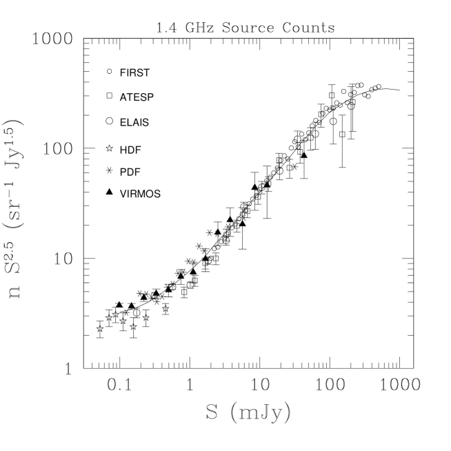
Figure 13: The normalised differential source counts. The abscissa gives the flux density (mJy) and the ordinate gives the differential number of sources normalised by $S^{2.5}$ (sr^-1 Jy^+1.5). With different symbols are reported source counts at 1.4 GHz from several surveys: the smaller open circles represent the counts from the FIRST survey (White et a. (1997)), the open squares are the counts from the ATESP survey (Prandoni et al. 2001a ), the larger open circles are the counts obtained by the survey ELAIS (Gruppioni et al. 1999b ;Ciliegi et al. (1999)), the stars are the counts from the HDF (Richards (2000)), the asterisks are the counts from the Phoenix Deep Survey (Hopkins et al. (1998)), the filled triangles are the counts obtained with the VIRMOS survey discussed in this paper. The solid lines is a best fit to a compilation of earlier deep surveys made by Katgert et al. (1988)

5.2 Completeness

In order to estimate the combined effects of noise, source extraction and flux determination techniques and resolution bias on the completeness of our sample, we constructed simulated samples of radio sources down to a flux level of 0.04 mJy, i.e. a factor of two lower than the minimum flux we used to derive the source counts (see Sect. 5.3). This allows to take into account also those sources with an intrinsic flux below the detection limit which, because of positive noise fluctuations, might have a measured flux above the limit. The simulated samples have been extracted from source counts with the integral size distribution derived in the previous section and described by a broken power law consistent with that observed.

Following these recipes, we simulated 9 samples, each of them with a number of sources above the detection limit similar to that observed in the real data (i.e. $\simeq 1000$). All the sources, including those below the detection limit, were randomly injected in the CLEANed sky images of the field and were recovered from the image and their fluxes were measured using the same procedures adopted for the real sources (see Sect. 4). The detected simulated sources were then binned in flux intervals. Finally, from the comparison between the number of simulated sources detected in each bin and the number of sources in the input simulated sample in the same flux bin we computed the correction factor $C$ to be applied to our observed source counts. In Table 3 we report the average correction factor $C$ for each flux density bin. As expected, the resolution bias significantly affects the first two flux density bins in the source counts. Our simulations tell us we are missing about 29% and 25% of sources in the first two flux density bins respectively. In the bins at higher flux the results of these simulations are consistent with no need for a correction. We therefore set $C=1.0$ for all these bins.

5.3 Source counts

In order to reduce possible problems near the flux limit and to avoid somewhat uncertain corrections in the steep part of the visibility area we constructed the radio sources counts considering only the 1013 sources with a flux density greater than 0.08 mJy ($i.e.$ we excluded the 41 sources with S$<$0.08 mJy). The 1.4 GHz source counts of our survey are summarised in Table 3. For each flux density bin, the average flux density, the observed number of sources, the differential source density (in sr^-1 Jy^-1), the normalised differential counts $nS^{2.5}$ (in sr^-1 Jy^1.5) with estimated Poissonian errors (as $n^{1/2}S^{2.5}$). In the last two columns we report the correction factor $C$ to be applied to our source counts to correct for incompleteness and the corrected integral counts (in deg^-2).

The normalised 1.4 GHz counts (column V) multiplied by the correction factor $C$ are plotted in Fig. 13 where, for comparison, the differential source counts obtained with other 1.4 GHz radio surveys are also plotted.

Our counts are in good agreement, over the entire flux range sampled by our data (0.08 - 10 mJy), with the best fit to earlier surveys (Katgert et al. (1988)). It is interesting to note that, because of the relatively good statistics of our data points over about two orders of magnitude in flux, our data clearly show the change in slope of the differential counts, occurring below 1 mJy. Fitting the VLA-VDF differential and integral counts with two power laws we obtain, for $S<0.6$ mJy:

$${dn\over ds}=(57.54\pm 1.07)\times S^{-2.28\pm 0.04}$$

and at higher fluxes, $S>0.6$ mJy:

$${dn\over ds}=(75.86\pm 1.08)\times S^{-1.79\pm 0.05}$$

where dn/ds is in deg^-1mJy^-1 e $S$ in mJy. At faint fluxes ($S<0.4$ mJy) the most relevant comparison is with the results obtained by Richards (2000) in his deep VLA survey of a region of about 40 x 40 arcmin around the Hubble Deep Field. In this flux range the statistics in our data (i.e. number of radio sources) is about four times higher than that in the HDF data and our derived counts are about 50% higher than those of Richards (see also Hopkins et al. (2002) for similar results). This is consistent with the fact, already noted by Richards, that the counts in the HDF region appear to be sistematically lower than those of other fields above 0.1 mJy. This difference is probably due to a combination of real field-to field variations and some possible incompleteness of somewhat extended sources in the high resolution HDF data ($2^{\prime\prime}$ beam). Indeed, lower resolution, deep Westerbork observations of a sub-area in the Hubble Deep Field region have detected a non-negligible number of sources which do not appear in Richards’ catalogue (Garrett et al. (2000)).

6 Conclusions

Using the VLA at 1.4 GHz we have observed a 1 deg² field centered on the VIRMOS Deep Field (RA=02:26:00 DEC=$-04$:30:00), imaging the whole area with uniform sensitivity and a resolution of 6 arcsec. We have investigated the effects of clean bias and bandwidth smearing on our observations confirming that the observing strategy and the data reduction procedure allow us to consider these effects negligible. A complete catalogue of 1054 radio sources down to a local $5\sigma$ limit ($\simeq 80$ $\mu$Jy) has been compiled. In order to assess the effects of random noise, source extraction technique and resolution bias on the completeness of our sample we have first derived the effective angular-size distribution using the sources in our sample in the range 0.4-1.0 mJy. Then we have generated a large sample of simulated sources using the derived angular-size distribution and extracted from source counts described by a broken power law consistent with that observed. These simulations allowed us to statistically correct ourc counts in the faintest flux bins. The final counts are in good agreement with the best fit to earlier surveys (Katgert et al. (1988)). In particular, our data clearly show a significant change in slope of the differential counts occurring below 1.0 mJy. The best fit slope in the range 0.08-0.6 mJy ($-2.28\pm 0.04$) is close to the Euclidean value. At faint fluxes ($S<0.4$ mJy), where we have a high statistics, our derived counts are about 50% higher than those of Richards (2000) in the HDF region. This is consistent with the fact, already noted by Richards, that the counts in the HDF region appear to be sistematically lower than those of other fields above 0.1 mJy

The same region of the sky has been target of deep ($I_{\rm AB}=25$), multicolor (UBVRIK) photometry observations. The photometric identification of most of the radio sources in the catalogue and planned spectroscopic observations during the VIRMOS Deep Field Survey will provide a unique opportunity to study the nature and properties of the $\mu$Jy source population.