Relativistic parsec–scale jets: II. Synchrotron emission

We calculate the optically thin synchrotron emission of fast electrons and positrons in a spiral stationary magnetic field and a radial electric field of a rotating relativistic strongly magnetized force–free jet consisting of electron-positron pair plasma. The magnetic field has a helical structure with a uniform axial component and a toroidal component that is maximal inside the jet and decreasing to zero towards the boundary of the jet. Doppler boosting and swing of the polarization angle of synchrotron emission due to the relativistic motion of the emitting volume are calculated. The distribution of the plasma velocity in the jet is consistent with the electromagnetic field structure. Two spatial distributions of fast particles are considered: uniform, and concentrated in the vicinity of the Alfvén resonance surface. The latter distribution corresponds to the regular acceleration by an electromagnetic wave in the vicinity of its Alfvén resonance surface inside the jet. The polarization properties of the radiation have been obtained and compared with the existing VLBI polarization measurements of parsec–scale jets in BL Lac sources and quasars. Our results give a natural explanation of the observed bimodality in the alignment between the electric field vector of the polarized radiation and the projection of the jet axis on the plane of the sky. We interpret the motion of bright knots as a phase velocity of standing spiral eigenmodes of electromagnetic perturbations in a cylindrical jet. The degree of polarization and the velocity of the observed proper motion of bright knots depend upon the angular rotational velocity of the jet. The observed polarizations and velocities of knots indicate that the magnetic field lines are bent in the direction opposite to the direction of the jet rotation.

1 Introduction

The jets from Active Galactic Nuclei are not uniform. They consist of a number of bright knots with fainter emission in between. It is well established that the nature of the radio emission from jets on kiloparsec and parsec scales is synchrotron radiation of relativistic nonthermal particles (Begelman et al. 1984). There is mounting observational evidence that jets in many AGNs are electron-positron rather than electron-proton. The spectral model of the jet radiation in a broad frequency range (from X-rays to radio), is described by Morrison & Sadun (1992), who pointed out that the 3C273 jet must be dominated by electron-positron pairs. Reynolds et al. (1996) used early VLBI observations of the M87 jet and self-absorbed core. They used the theory of synchrotron self-absorption to put a constraint on the electron density in the core and concluded that the core of M87 is likely to be e⁺e^- pair plasma. A similar method was used by Hirotani et al. (1999) and Hirotani et al. (2000) to reveal that the components in the jets of 3C279 and 3C345 are also dominated by pair plasma. Observations of circular polarization of radio emission from 3C279, 3C273, 3C84 and PKS0528+134 (Wardle et al., 1998) support the same conclusion. However, there are also indications that jets in Optically Violently Variable quasars cannot consist solely of e⁺e^- pairs because they would produce much larger soft X-ray luminosities than are observed. On the other hand, models with jets consisting solely of proton-electron plasma are excluded, since they predict much weaker nonthermal X-radiation than observed in Optically Violently Variable quasars (Sikora & Madejski, 2000). The in situ acceleration of relativistic particles seems unavoidable because high synchrotron losses prevent relativistic particles from streaming out of the central engine to the distances of bright knots (Begelman et al. 1984; Röser & Meisenheimer 1991). There are several possible mechanisms of particle acceleration inside knots. The acceleration can be by shocks (Blandford & Eichler 1987), by turbulent electromagnetic fields (Manolakou, Anastasiadis & Vlahos 1999) and by magnetic reconnection (Romanova & Lovelace 1992; Blackman 1996). Another possible mechanism of particle acceleration is the acceleration by organized electromagnetic fields which are the eigenmodes of the jet as a whole. These modes can be excited as a result of non-stationary processes in the central engine. The energy can be transmitted by such global waves along the jet to large distances without noticeable attenuation.

The acceleration is most effective if resonances of the waves with the mean stream take place (Beresnyak et al. 2002). The resonance with Alfvén waves occurs when $\omega^{\prime}=k_{\|}^{\prime}c$, where $\omega^{\prime}$ and $k_{\parallel}^{\prime}$ are the frequency and the projection of the wave vector on the magnetic field in the plasma rest frame. When the specific energy density and pressure of the plasma are much less than the energy density of the magnetic field, The Alfvén velocity is equal to the speed of light in vacuum $c$. The resonance condition is fulfilled on a specific magnetic surface and, in the case of a cylindrical jet, at a definite distance from the axis. In the vicinity of that surface the magnetic and electric fields of the wave reach large magnitudes. The resonances occur for nonaxisymmetric modes of global waves and the position and width of the resonances depend on the structure of the ordered helical magnetic field. Both electrons and positrons are subject to drifting out of the region of the strong electric field of the wave near the resonance due to the non-uniformity of the electric field. When moving to a region of weak electric field, particles gain energy. This energy is taken from the energy of the wave, which is an eigenmode in the jet, and the eigenmode decays. Beresnyak at al. (2002) considered this mechanism of particle acceleration. Drift approximation was used to describe the motion of a particle in the electric field of the wave. Synchrotron losses and isotropization of the particle distribution by plasma instabilities were taken into account. Plasma instabilities are excited by accelerated particles if the distribution function is anisotropic in momentum space, and act to conceal any anisotropy in the particle distribution. Acceleration process and synchrotron losses taken together yield a power law energy spectrum of ultra-relativistic electrons and positrons with an index varying between $2$ and $3$ depending upon the initial energy of the injected particles. This is consistent with the typical spectral indices of radio emission observed in parsec–scale jets.

The polarization of synchrotron emission in knots is very sensitive to the geometry of the helical large scale magnetic field. Indeed, VLBI observations provide evidence for the polarized emission in knots and in the space between knots (Gabuzda 1999a; Hutchison et al. 2001). This is indicative of the existence of a large scale magnetic field all over the jet rather than concentrated in separate knots. In the general case a helical magnetic field has poloidal and toroidal components. The toroidal component arises due to the axial electric current in the jet. If the current inside the jet is closed (no net jet electric current), that is the electric current flows in different directions at different radii in the jet, then the toroidal magnetic field must be small at the boundary of the jet and only the axial component of the magnetic field will remain. The change of the direction of the magnetic field from toroidal close to the jet axis to axial on the periphery was inferred from the VLBI polarization measurements in blazar 1055+018 (Attridge et al. 1999). The concept of an intrinsic large-scale helical magnetic field is the simplest model of the jet and does not require additional processes of amplification or generation of azimuthal and axial components of the magnetic field in shocks or shearing layers at the jet boundary.

The polarization of synchrotron emission of parsec scale jets is being studied by few groups (Gabuzda 1999b, 2000; Leppänen at al. 1995; Lister 2001). We use observational data to compare with our calculations of polarization in a model of a force–free strongly magnetized relativistic rotating jet. We calculate the polarization of synchrotron radiation in the helical field geometry (Sect. 2). In Sect. 3 we expand our calculations to include the Doppler boosting effect and swing of the polarization angle due to relativistic motion and rotation of the plasma in the jet. We also compare the observed apparent velocities of knots with the velocities given by our model of propagation of spiral perturbations in a cylindrical jet. As it was shown by Istomin & Pariev (1994, 1996) there exist so-called standing modes among eigenmodes in jets ($v_{\rm group}=0$) which do not propagate with finite velocity along the jet but are only subject to diffuse spreading and, therefore, their amplitude is maximal. The phase velocity of these modes is greater than the speed of light. The crests of the wave move along the jet with superluminal velocity causing acceleration of the particles on the Alfvén resonance surface. These regions can be the objects which are seen as bright knots with typical sizes of the order of the wavelength of the standing wave, which is about the radius of the jet.

2 Synchrotron emission.

Let us now consider synchrotron emission of accelerated particles in a cylindrical force–free jet with a spiral magnetic field. For cylindrical jet the stationary configuration of fields is (Istomin & Pariev 1994):

$${\bf B}=B_{z}{\bf e}_{z}+B_{\phi}{\bf e}_{\phi};\quad B_{\phi}=\pm\frac{\Omega^{F}r}{c}B_{z},$$ (1)

where $r,\phi,z$ are cylindrical coordinates. The profile of the poloidal magnetic field $B_{z}$ is taken to be uniform across the jet. The velocity of plasma can be written as

$${\bf u}=K{\bf B}+\Omega^{F}r{\bf e}_{\phi},$$ (2)

where $\Omega^{F}$ is the angular rotational velocity of the magnetic field lines and $K{\bf B}$ is the component of the velocity parallel to the magnetic field. The electric field is induced due to the motion of highly conducting plasma across the magnetic field and is equal to

$${\bf E}=-\frac{\Omega^{F}r}{c}[{\bf e}_{\phi}{\times\bf B}].$$ (3)

In components

$${\bf B}=(0,\pm\Omega^{F}r/c,1)B_{z},$$ (4)

$${\bf E}=(-\Omega^{F}r/c,0,0)B_{z},$$ (5)

$${\bf u}=(0,\Omega^{F}r(1\pm KB_{z}/c),KB_{z}).$$ (6)

Here $\Omega^{F}$ and $K$ are functions of $r$, and $B_{z}$ does not depend on $r$. The stationary electric field, which has an absolute value of $\Omega^{F}rB_{z}/c$, is not small compared to the magnetic field when $\Omega^{F}r\sim c$. The rotation velocity $\Omega^{F}r$ can exceed the speed of light; nevertheless $u$ remains less than $c$ due to the existence of the predominantly toroidal magnetic field. This can be achieved by appropriate choice of the parameter $K$. The natural requirement that the total poloidal current is closed inside the jet and that the total electric charge of the jet is zero implies that $\Omega^{F}$ must vanish at the boundary of the jet $r=R$ (Istomin & Pariev 1994). Besides this requirement, the dependence $\Omega^{F}=\Omega^{F}(r)$ should be determined by the conditions at the jet origin. An arbitrary parameter $K(r)$ in expression (2) for the plasma velocity determines the radial profile of the longitudinal velocity. $K(r)B_{z}$ is the velocity along the magnetic field which is not related to the rotation. We choose a velocity ${\bf u}$ which minimizes the kinetic energy of the plasma in the stationary reference frame

$${\bf u}=\frac{(0,\Omega^{F}r,\mp(\Omega^{F}r)^{2}/c)}{1+(\Omega^{F}r/c)^{2}}.$$ (7)

It is probable that the plasma moves with that velocity in real jets originating near black holes (Frolov & Novikov 1998). The geometry of the magnetic and electric fields and the flow in the jet are illustrated in Fig. 1.

In accordance with our theory of particle acceleration inside a force–free relativistic jet (Beresnyak et al. 2002) we consider the distribution function of emitting particles to be isotropic in momentum and power law in energy

$$dn=K_{e}{\cal E}^{-\zeta}d{\cal E}dVd\Omega_{\bf p}$$ (8)

Here $dn$ is the number of particles in the energy interval ${\cal E},{\cal E}+d{\cal E}$, $dV$ is the elementary volume, $d\Omega_{\bf p}$ is the elementary solid angle in the direction of the particle momentum ${\bf p}$, $K_{e}=K_{e}(r)$, $\zeta=\mbox{constant}$. We will assume that ultrarelativistic particles are distributed according to Eq. (8) in the frame moving with the plasma with the velocity ${\bf u}$, Eq. (7). One needs to know the distribution of the density of relativistic particles over the jet radius $K_{e}(r)$. Several mechanisms for particle acceleration inside jets have been considered previously. The possible processes are acceleration by the shocks in the supersonic flow of mass-loaded jets (Blandford & Eichler 1987) and acceleration due to magnetic reconnection near the neutral layers of the poloidal magnetic field (Romanova & Lovelace 1992). Usually, the distribution of fast particles inside the jet was assumed to be uniform (Laing 1981) or smoothly varying with the radius in the jet (Königl & Choudhuri 1985). According to our mechanism of particle acceleration (Beresnyak et al. 2002), relativistic particles are accelerated close to the Alfvén resonance surface $r=r_{A}$ and are concentrated near the same surface. The position of the Alfvén resonance in a force–free jet is determined by the condition

$$kc-\omega+2m\Omega^{F}(r_{A})-\left(\frac{\Omega^{F}(r_{A})r_{A}}{c}\right)^{2}(\omega+kc)=0,$$ (9)

where $\omega=\omega_{m}(k)$ is the eigenfrequency of the perturbation of the magnetic field $\propto\exp(-i\omega t+ikz+im\phi)$ with the wavenumber $k$ along the axis of the jet and azimuthal number $m$. We will consider two cases for the spatial distribution of particles, namely, uniform in the jet volume and concentrated close to the Alfvén resonant surface $r=r_{A}$.

The influence of the plasma on the emission of relativistic $e^{-}$ and $e^{+}$ is neglected in the present work. Absorption and reabsorption are also not taken into account. Electrons and positrons are accelerated in the same way near Alfvén resonance and have the same distribution function. Therefore, the Faraday rotation effect is absent as well as intrinsic depolarization inside the jet. VLBI polarization measurements are done at frequencies in the range $1\,\mbox{GHz}$ to $100\,\mbox{GHz}$. Synchrotron self-absorption is very small at GHz frequencies and higher frequencies. For $B\sim 10^{-2}\,\mbox{G}$, $n\sim 0.1\,\mbox{cm}^{-3}$, and $\zeta\approx 2.5$ an order of magnitude estimate for the synchrotron self-absorption coefficient is $\displaystyle\kappa_{s}=(5\cdot 10^{3}\,\mbox{pc})^{-1}\left(\nu/1\,\mbox{GHz}\right)^{-2-\zeta/2}$ (e.g., Zhelezniakov 1996). The corresponding optical depth through the $1\,\mbox{pc}$ jet is only $2\cdot 10^{-4}$. The typical energy of particles emitting in this frequency range in $10^{-2}\,\mbox{G}$ magnetic field is $100\,\mbox{MeV}$ to $1\,\mbox{GeV}$. Conversion of linear polarized radio waves into circular polarized (Cotton–Mouton effect) is also small. For both thermal and relativistic power law particle distributions with $\zeta\approx 2.5$ and a minimum Lorentz factor $\sim 10$ the estimate for the conversion coefficient is $\displaystyle\kappa_{c}=(500\,\mbox{pc})^{-1}\left(\nu/1\,\mbox{GHz}\right)^{-3}$ (Sazonov 1969). This is too small to influence the transfer of linear polarization inside the jet, but can be the source for a small, at the level of a fraction of per cent, circular polarization. We focus on linear polarization in this work.

At first, we neglect Doppler boosting, i.e. assume that ${\bf u}=0$ for the purpose of the calculation of the synchrotron radiation. However, the magnetic field will still be given by formulae (1) with nonvanishing $\Omega^{F}$. In Sect. 3 we take into account Doppler boosting with velocity ${\bf u}$ consistent with the field configuration according to expressions (4–6) and see that the proper consideration of the Doppler effect leads to a marked change in polarization. When no Doppler effect is considered, the Stokes parameters are obtained by integration along the line of sight passing through the region filled with relativistic particles inside the jet (e.g., Ginzburg 1989). Let us denote the angle between the axis of the jet (the direction of the axial magnetic field $B_{z}$) and the observer by $\theta$, such that $\theta=0$ when $B_{z}$ points exactly at the observer, $\theta=\pi/2$ when the line of sight of the observer is perpendicular to the direction of the jet axis, and $\theta=\pi$ when the $B_{z}$ points exactly away from the observer. The azimuthal angle $\phi$ is measured from the plane containing the observer and the jet axis; $\phi$ increases from $0$ to $2\pi$ in anticlockwise direction if viewed from the positive direction of axial magnetic field $B_{z}$. Let us denote the distance between the line of sight and the jet axis by $h$ and the radius of the jet by $R$. We will take $h$ as a signed quantity: $h>0$ for lines of sight passing in the sector $0<\phi<\pi$, $h<0$ for the lines of sight passing in the sector $\pi<\phi<2\pi$. We will parametrize integration along the line of sight by integration in $\phi$ keeping the value of $h$ constant. We define Stokes parameters in the usual way with reference to the rectangular coordinates in the plane of the sky with the $x$–axis oriented along the projection of the jet axis on the plane of the sky and the $y$–axis orthogonal to the $x$–axis in the anticlockwise direction. This geometry and the angles are illustrated in Fig. 1. Considering the geometry described above we obtain the following expressions for the Stokes parameters

$$I=\frac{\zeta+7/3}{\zeta+1}k(\nu)\int\limits_{\phi_{1}}^{\phi_{2}}|B_{\perp}|^{(\zeta+1)/2}\frac{h}{\sin\theta\sin^{2}\phi}\,d\phi,$$ (10)

$$Q=k(\nu)\int\limits_{\phi_{1}}^{\phi_{2}}\frac{|B_{\perp}|^{(\zeta+1)/2}}{|B_{\perp}|^{2}}\frac{[B_{\phi}^{2}\cos^{2}\phi-(B_{z}\sin\theta+B_{\phi}\sin\phi\cos\theta)^{2}]h}{\sin\theta\sin^{2}\phi}\,d\phi,$$ (11)

$$U=-2k(\nu)\int\limits_{\phi_{1}}^{\phi_{2}}\frac{|B_{\perp}|^{(\zeta+1)/2}}{|B_{\perp}|^{2}}B_{\phi}\cos\phi(B_{z}\sin\theta+B_{\phi}\sin\phi\cos\theta)\frac{h}{\sin\theta\sin^{2}\phi}\,d\phi,$$ (12)

$$V=0,$$ (13)

where $B_{\perp}$ is the component of the magnetic field perpendicular to the line of sight. The integration limits are $\displaystyle\phi_{1}=\pi\,\mbox{sgn}\,h-\arcsin\frac{h}{R},\quad\phi_{2}=\arcsin\frac{h}{R}$. The value of $k(\nu)$ is a function of the observed frequency $\nu$ of the radiation

$$k(\nu)=\frac{\sqrt{3}}{4}\Gamma\left(\frac{3\zeta-1}{12}\right)\Gamma\left(\frac{3\zeta+7}{12}\right)\frac{e^{3}}{m_{e}c^{2}}\left[\frac{3e}{2\pi m_{e}^{3}c^{5}}\right]^{(\zeta-1)/2}\nu^{-(\zeta-1)/2}\frac{K_{e}}{D^{2}},$$

where $D$ is the distance between the source and the observer, $e$ and $m_{e}$ are the charge and mass of an electron, and $\Gamma$ is the Euler gamma-function.

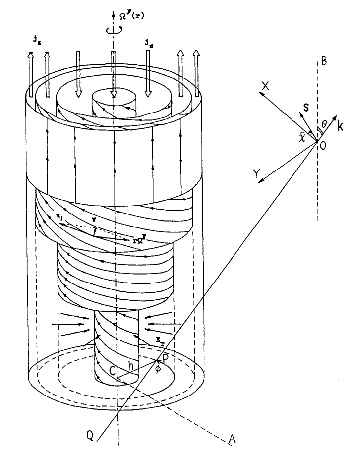
Figure 1: The scheme illustrating the geometry of the jet and of the polarization observations. The jet boundary for $r=R$ and three magnetic tubes for $r=R/4$, $2R/3$ and $9R/10$ are shown for uniform $B_{z}$ and angular velocity profile (18) with $\Omega=10$. The magnetic field lines are spiralling on a magnetic tube. Since $\Omega^{F}(R)=0$, the total current through the jet is equal to zero and the magnetic field is purely poloidal both at the boundary and at the axis of symmetry. The density of the poloidal current $j_{z}$ is negative when $r<R/\sqrt{2}$ and positive when $R>r>R/\sqrt{2}$. The electric field ${\bf E}$ induced by jet rotation is radial. The plasma velocity ${\bf v}$ along the magnetic tube consists of two components: rotation with angular velocity $\Omega^{F}(r)$, and motion along the magnetic field lines with a speed ${\bf v}_{\parallel}=K{\bf B}$. A line of sight OQ passes through the jet at a closest distance $\mbox{CP}=h$ from the jet axis. The line CA is parallel to the plane containing the observer and the jet axis. OXY is a rectangular coordinate system on the plane of the sky of the observer, OX is in the plane containing the observer and the jet axis. The line OB is parallel to the jet axis, and the wave vector of a photon ${\bf k}$ makes an angle $\theta$ with the line OB and the jet axis. Vector ${\bf s}$ is a unit vector in the direction of the electric vector of the polarized component. Vector ${\bf s}$ is in the plane OXY and makes an angle ${\tilde{\chi}}$ with OX.

We denote the position angle of the electric field vector in the plane of the sky by $\tilde{\chi}$. The angle $\tilde{\chi}$ is measured clockwise from the direction parallel to the projection of the jet axis on the plane of the sky and $0<\tilde{\chi}<\pi$ (see Fig. 1). For ultra-relativistic particles $V=0$, and the emission has only linear polarization. The degree of polarization of the observed radiation is expressed as $\Pi=\sqrt{Q^{2}+U^{2}}/I$, the resultant position angle of the electric field $\tilde{\chi}_{\rm res}$ measured by the observer is found from

$$\cos 2\tilde{\chi}_{\rm res}=\frac{Q}{\sqrt{Q^{2}+U^{2}}},\quad\sin 2\tilde{\chi}_{\rm res}=\frac{U}{\sqrt{Q^{2}+U^{2}}},\quad 0\leq\tilde{\chi}_{\rm res}<\pi.$$

It is seen that when one replaces the variable $\phi$ by $\pi-\phi$ in expression (12), $U$ changes its sign and, therefore, $U=0$. Consequently, if $Q>0$ then $\tilde{\chi}_{\rm res}=0$, if $Q<0$ then $\tilde{\chi}_{\rm res}=\pi/2$. Thus, the observed electric field vector is either parallel or perpendicular to the jet axis on the plane of sky. This may account for the bimodal distribution of the observed $\tilde{\chi}_{\rm res}$ (Gabuzda et al. 1994). Now let us integrate expressions (10) and (11) for $I$ and $Q$ over parameter $h$ in order to obtain the total radiation flux and polarization per unit length of the jet image on the sky. Assuming uniform emissivity over the jet volume, $B_{z}=\mbox{constant}$ and $B_{\phi}=B_{z}\Omega^{F}r/c$ expressions for $I$ and $Q$ from the unit jet length become

$$I=\frac{\zeta+7/3}{\zeta+1}k(\nu)\int\limits_{-R}^{R}dh\int\limits_{\phi_{1}}^{\phi_{2}}|B_{\perp}|^{(\zeta+1)/2}\frac{h}{\sin\theta\sin^{2}\phi}\,d\phi,$$ (14)

$$Q=k(\nu)\int\limits_{-R}^{R}dh\int\limits_{\phi_{1}}^{\phi_{2}}|B_{\perp}|^{(\zeta-3)/2}\frac{[{\Omega^{F}}^{2}r^{2}\cos^{2}\phi-(c\sin\theta+\Omega^{F}r\sin\phi\cos\theta)^{2}]B_{z}^{2}h}{c^{2}\sin\theta\sin^{2}\phi}\,d\phi.$$ (15)

For $\zeta=3$ expressions (14) and (15) are reduced to the form

$$I=\frac{4}{3}k(\nu)B_{z}^{2}\frac{\pi}{\sin\theta}\int\limits_{0}^{R}2r\left[\sin^{2}\theta+\frac{{\Omega^{F}}^{2}r^{2}}{c^{2}}\left(1-\frac{1}{2}\sin^{2}\theta\right)\right]\,dr,$$ (16)

$$Q=k(\nu)B_{z}^{2}\pi\sin\theta\int\limits_{0}^{R}\left(\frac{{\Omega^{F}}^{2}r^{2}}{c^{2}}-2\right)r\,dr.$$ (17)

From the above we see that in the case $\zeta=3$ the sign of $Q$ does not depend on $\theta$ since $\sin\theta>0$ for any $0<\theta<\pi$. The sign of $Q$ is determined by the function $\Omega^{F}(r)$ only.

Let us choose a particular dependence of $\Omega^{F}(r)$ satisfying the requirements $\Omega^{F}(R)=0$ and $d\Omega^{F}/dr=0$ at $r=0$. At present, there is no well established theory which would predict $\Omega^{F}(r)$. Therefore, we choose the simplest monotonic profile satisfying the physical requirements above:

$$\Omega^{F}=\Omega\frac{c}{R}\left(1-\left(\frac{r}{R}\right)^{2}\right),$$ (18)

where $\Omega$ is a dimensionless parameter. Although the exact position of $r_{A}$, the ratio of $B_{\phi}/B_{z}$ at $r_{A}$ and the velocity of the flow in the vicinity of $r_{A}$ (properties which determine the observed polarization) are all dependent on the particular choice of $\Omega^{F}(r)$ profile, it is the magnitude of the angular rotational velocity which influences all these parameters most significantly. A qualitative difference may appear if the profile of $\Omega^{F}$ is non-monotonic, such that many Alfvén resonant surfaces will exist inside the jet. In this work we limit our consideration to variation of parameter $\Omega$ only, but keeping the radial profile of $\Omega^{F}$ monotonic and given by expression (18). Then, for $\zeta=3$ using expressions (16) and (17) one obtains the degree of polarization $\Pi$

$$\Pi=\frac{3}{4}\frac{\displaystyle\left(\frac{\Omega^{2}}{24}-1\right)\sin^{2}\theta}{\displaystyle\sin^{2}\theta+\frac{\Omega^{2}}{12}\left(1-\frac{1}{2}\sin^{2}\theta\right)}.$$

If $|\Omega|>2\sqrt{6}$, then $Q>0$ and $\tilde{\chi}_{\rm res}=0$, i.e. the electric vector of the polarized emission is parallel to the projection of the jet axis on the plane of the sky. This does not mean, however, that the orientation of the magnetic field in the jet is purely perpendicular to the jet axis. Clearly, one can see from Eq. (1) that the poloidal magnetic field is comparable to the toroidal field. If $0<|\Omega|<2\sqrt{6}$ then $Q<0$ and $\tilde{\chi}_{\rm res}=\pi/2$, i.e. the electric vector of the polarized emission is perpendicular to the projection of the jet axis on the plane of sky. Again, this does not mean that the orientation of the magnetic field in the jet is purely parallel to the jet axis. The toroidal magnetic field vanishes only if $\Omega=0$, otherwise the toroidal magnetic field is comparable to the poloidal magnetic field. This simplified analytical calculation shows that one needs to be very careful when interpreting the polarization measurements in terms of the orientation of the magnetic field.

Eqs. (14) and (15) were integrated numerically for the dependence $\Omega^{F}(r)$ given by expression (18) and $\zeta=2.1$, which corresponds to the power law index in the spectrum of synchrotron emission of $(\zeta-1)/2=0.55$, the mean observed value for extragalactic jets (Scheuer 1984). The results are presented in Fig. 2. Positive values of the degree of polarization correspond to $\tilde{\chi}_{\rm res}=0$, negative to $\tilde{\chi}_{\rm res}=\pi/2$. In the case $\Pi=0$ the radiation is entirely unpolarized. Note also that in the nonrelativistic consideration $\Pi(180^{0}-\theta)=\Pi(\theta)$ for any value of $\theta$.

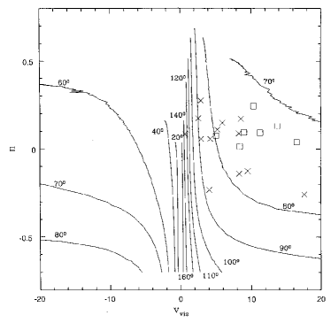
Figure 2: Dependences of linear polarization $\Pi$ on angular rotational velocity $\Omega$ (left panel) and on visual velocity of knots $v_{\rm vis}$ (right panel) for fundamental axisymmetric mode $m=0$. $\Pi>0$ when the electric field vector is oriented parallel to the jet axis, $\Pi<0$ when the electric field vector is oriented perpendicular to the jet axis. $v_{\rm vis}>0$ means that the observed motion of knots is direct, $v_{\rm vis}<0$ means reversal motion. Crosses are for the BL Lac objects and squares are for the quasars listed in Table 1.

Istomin & Pariev (1996) presented a hypothesis that knots observed in jets can be the manifestation of the “standing wave” phenomenon. If one knows the dispersion curves $\omega=\omega(k)$ and wavenumbers $k_{\rm min}$ at which $d\omega/dk=0$ for perturbations, one can calculate the velocity of moving crests of the “standing wave” as $v_{\rm phas}=\omega_{\rm min}(k_{\rm min})/k_{\rm min}$ and corresponding observed velocity $\displaystyle v_{\rm vis}=\frac{v_{\rm phas}\sin\theta}{1-v_{\rm phas}\cos\theta/c}$. Note also that changing the sign of $B_{\phi}$ in Eq. (4) is equivalent to changing the sign of $\Omega^{F}$, since $I$ and $Q$ depend only on $B_{z}$ and $B_{\phi}$ and not on $u$ or $E_{r}$. In Fig. 2 we present the relations of the polarization $\Pi$ of the jet emission and $v_{\rm vis}$ obtained in the case of $\Omega$ changing from $0$ to $100$ for some angles $\theta$. We also plotted observational points for jets in BL Lac objects and quasars for which we were able to find both polarization and proper motion measurements in the literature and which are listed in Table 1. For each object we averaged the degree of polarization and observed velocity over all bright knots observed in a particular object excluding a few knots, for which peculiarity was indicated in the original references. This procedure might be very questionable although because of the lack of observations of the emission from the space between knots on parsec scale we had nothing better. The polarization measurements also depend on the frequency of observations. Specifically, different observations of quasars give very different values of the polarization of the knots at centimetre and millimetre wavelengths. Numbers for $v_{\rm vis}$ were calculated assuming a Hubble constant $H=65h\mbox{km/s}\cdot\mbox{Mpc}$

Table 1: Polarization degrees and velocities of knots in BL Lac objects and quasars

Class	Source	$\Pi\,$,%	$v_{\rm vis}h/c$	References
BL Lac	0138-097	8.8	8.5	1
BL Lac	0454+844	8.5	0.92	1
BL Lac	0735+178	-14.	8.5	1
BL Lac	0828+493	-12.5	9.7	1
BL Lac	0851+202	-23.3	4.3	1
BL Lac	0954+658	17.2	8.8	1
BL Lac	1418+546	5.6	3.2	1
BL Lac	1732+389	-25.9	17.8	1
BL Lac	1803+784	27.5	3.2	2,3
BL Lac	1823+568	14.9	6.2	1
BL Lac	2007+777	5.6	4.5	1
BL Lac	2200+420	11.	5.5	1
quasar	0212+735	1.4	8.6	2,3
quasar	0836+710	2.2	21.7	2,3
quasar	0906+430	7.5	5.3	2,3
quasar	1055+018	9.5	9.23	4
quasar	1308+326	3.8	16.8	5
quasar	3C345	11.	29.3	2,3
quasar	1642+690	13.	14.0	2,3
quasar	1928+738	9.3	11.5	2,3
quasar	3C380	24.4	10.6	2,3

RefeRences.— (1) Gabuzda et al. (2000), (2) Lister et al. (2001), (3) Lister (2001), (4) Lister et al. (1998), (5) Gabuzda & Cawthorne (1993)

In the case of accelerated particles concentrated very close to the Alfvén surface $r=r_{A}$ expressions (14) and (15) can be reduced to integrals in $\phi$ only, while $r=r_{A}$.

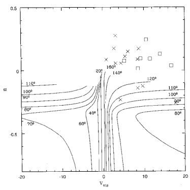
Figure 3: The same as in Fig. 2 but emitting particles are concentrated close to the Alfvén resonance surface, $m=1$ fundamental mode. The curves are plotted only for $0.7<\Omega<4.9$, when the Alfvén resonance exists for the $m=1$, $k=k_{\rm min}$ mode.

Since for axisymmetric modes ($m=0$) always $|\omega_{\rm min}|>|k_{\rm min}|c$ (Istomin & Pariev 1994) one can see from the expression (9) that the Alfvén resonance does not exist for axisymmetric modes. Therefore, there should be no particle acceleration for this mode. The next most important modes are $m=1$ and $m=-1$. Since none of the quantities $k_{\rm min}$, $\omega_{\rm min}$ or $\Pi$ changes when $m$ changes to $-m$ and $\Omega^{F}$ to $-\Omega^{F}$, it is enough to consider only positive $m=1$ and all values of $\Omega^{F}$ (positive and negative). Polarization $\Pi$ versus $v_{\rm phas}$ for this case is plotted in Fig. 3 as well as observational points. We plotted $v_{\rm phas}$ only for the first non-axisymmetric fundamental mode $m=1$ which is expected to be excited more easily than higher modes with $m>1$. Observations of the parsec scale jet in BL Lac object 0820+225 (Gabuzda et al. 2001) show the S–like shape which can be attributed to the mode $m=1$. The polarization curves are plotted only for values of $\Omega$ at which the Alfvén resonance $r=r_{A}$ is present inside the jet. As previously, $\Omega^{F}(r)$ is given by expression (18) and $\zeta=2.1$. It is seen that in the case of uniform particle distribution across the jet (Fig. 2), curves for $\theta$ changing from $120^{\circ}$ to $70^{\circ}$ are located in the region where points from observations of BL Lac object (crosses) and quasars (squares) are. However, the polarization curves for emitting particles concentrated on the Alfvén resonance surface (Fig. 3), as is the case for our acceleration mechanism, do not match the observations of quasars. It is seen from Fig. 3 that the electric field vector is always oriented perpendicular to the jet axis unlike the case with uniform distribution of relativistic particles across the jet. The reason for this difference is that the Alfvén resonance surface exists only for moderate values of $\Omega$, when the toroidal magnetic field is not strong enough to cause the $\tilde{\chi}_{\rm res}$ to become oriented parallel to the projection of the jet axis on the plane of the sky.

3 Relativistic Doppler boosting effect on polarization

Now let us make more realistic calculations taking into account Doppler boosting and the presence of a strong electric field. As was first pointed out by Blandford & Königl (1979) the effect of relativistic aberration of light causes a swing of the direction of polarization of synchrotron emission when the source is Doppler boosted. This is due to the fact that the electric vector of the polarized component of the wave must remain orthogonal to the wave vector. We will denote values measured in the plasma rest frame by primes. Let us find the transformation rules for the polarization tensor $J_{\alpha\beta}=<E_{\alpha}E_{\beta}^{*}>$ from the local reference frame of the small emitting volume moving with velocity ${\bf u}$ to the observer reference frame. Here $<\ldots>$ is the averaging over realizations of electric wave fields. The Stokes parameters are components of the polarization tensor $J_{\alpha\beta}=\frac{1}{2}\left(\begin{array}[]{cc}I+Q&U\\ U&I-Q\end{array}\right).$ We denote the local Cartesian coordinates in the source frame by $x^{\prime}y^{\prime}z^{\prime}$ and the Cartesian coordinates in the observer frame by $xyz$. The transformation can be done by directly using the transformation formulae for the electric and magnetic fields of the wave (Cocke & Holm 1972). The result is

$$J_{\alpha\beta}=J^{\prime}_{\alpha^{\prime}\beta^{\prime}}\frac{1-u^{2}/c^{2}}{(1-u/c\cos\delta)^{2}}.$$ (19)

Here we denote by $\delta$ the angle between velocity ${\bf u}$ of the source and the direction toward observer ${\bf k}$ measured in the observer frame; correspondingly, $\delta^{\prime}$ is the same angle but measured in the source frame. Thus, the polarization ellipse in the observer frame is obtained from the polarization ellipse in the source frame by rotation by the angle $\delta-\delta^{\prime}$ in the plane containing the direction to the observer ${\bf k}$ and ${\bf u}$. Therefore, the degree of polarization is not changed, which is obvious. The Stokes parameters for the radiation of one particle are expressed through the radiation flux with two main directions of polarization $p^{(1)}_{\nu^{\prime}}$ and $p^{(2)}_{\nu^{\prime}}$ by the formulae $I^{\prime}=p^{(1)}_{\nu^{\prime}}+p^{(2)}_{\nu^{\prime}}$, $Q^{\prime}=(p^{(1)}_{\nu^{\prime}}-p^{(2)}_{\nu^{\prime}})\cos 2\tilde{\chi}^{\prime}$ , $U^{\prime}=(p^{(1)}_{\nu^{\prime}}-p^{(2)}_{\nu^{\prime}})\sin 2\tilde{\chi}^{\prime}$, where $\tilde{\chi}^{\prime}$ is the position angle of the electric vector of polarized radiation in the reference frame comoving with the emitting volume (Ginzburg 1989). Then, $p^{(1)}_{\nu^{\prime}}$ and $p^{(2)}_{\nu^{\prime}}$ are transformed to the observer frame as

$$p^{(1)}_{\nu}=p^{(1)}_{\nu^{\prime}}\frac{d\nu^{\prime}}{d\nu}\frac{1-u^{2}/c^{2}}{(1-u/c\cos\delta)^{2}},\quad p^{(2)}_{\nu}=p^{(2)}_{\nu^{\prime}}\frac{d\nu^{\prime}}{d\nu}\frac{1-u^{2}/c^{2}}{(1-u/c\cos\delta)^{2}}.$$

Therefore the intensity in the observer frame integrated along the line of sight is

$$I(\nu,{\bf k})=\int(p^{(1)}_{\nu^{\prime}}(\nu^{\prime},{\cal E}^{\prime},{\bf L},\chi^{\prime},\psi^{\prime})+p^{(2)}_{\nu^{\prime}}(\nu^{\prime},{\cal E}^{\prime},{\bf L},\chi^{\prime},\psi^{\prime}))\times$$

$$\frac{d\nu^{\prime}}{d\nu}\frac{1-u^{2}/c^{2}}{(1-u/c\cos\delta)^{2}}K_{e}{{\cal E}^{\prime}}^{-\zeta}\frac{dV^{\prime}}{dV}d{\cal E}^{\prime}d\Omega_{{\bf p}^{\prime}}dL,$$

where $dL$ is the element of length along the line of sight, $\chi^{\prime}$ is the angle between the momentum of the particle and the magnetic field vector, $\psi^{\prime}$ is the angle between the direction of radiation and the cone formed by the velocity vector of the particle rotating around the magnetic field line, both measured in the frame comoving with the fluid element. We will integrate over the momenta in the plasma rest frame while integrating over the space coordinates in the observer frame. Integration over the solid angle $\Omega_{{\bf p}^{\prime}}$ in the momenta space in a comoving frame may be done analogous to the usual case of synchrotron emission of ultra-relativistic particles, when there is no electric field ${\bf E=-u\times B}$. Integration over $\Omega_{{\bf p}^{\prime}}$ and ${\cal E}^{\prime}$ leads to (Ginzburg 1989)

$$I(\nu,{\bf k})=\frac{\zeta+7/3}{\zeta+1}k(\nu)\int\left(\frac{1-u/c\cos\delta}{\sqrt{1-u^{2}/c^{2}}}\right)^{-\frac{\zeta-1}{2}}(B^{\prime}\sin\chi^{\prime})^{\frac{\zeta+1}{2}}\frac{dL}{1-u/c\cos\delta}.$$ (20)

Here $\displaystyle\nu^{\prime}=\nu\frac{1-u/c\cos\delta}{\sqrt{1-u^{2}/c^{2}}}$, ${\bf B^{\prime}}$ is the magnetic field in the emitter frame. The expressions for $Q$ and $U$ can be obtained in a similar way. The result is

$$Q(\nu,{\bf k})=k(\nu)\int{\left(\frac{1-u/c\cos\delta}{\sqrt{1-u^{2}/c^{2}}}\right)}^{-\frac{\zeta-1}{2}}(B^{\prime}\sin\chi^{\prime})^{\frac{\zeta+1}{2}}\frac{\cos 2\tilde{\chi}\,dL}{1-u/c\cos\delta},$$ (21)

$$U(\nu,{\bf k})=k(\nu)\int{\left(\frac{1-u/c\cos\delta}{\sqrt{1-u^{2}/c^{2}}}\right)}^{-\frac{\zeta-1}{2}}(B^{\prime}\sin\chi^{\prime})^{\frac{\zeta+1}{2}}\frac{\sin 2\tilde{\chi}\,dL}{1-u/c\cos\delta}.$$ (22)

The component of the magnetic field perpendicular to the momentum of the particle in the comoving frame, $B^{\prime}\sin\chi^{\prime}$, is obtained by applying the transformation rules

$$B^{\prime 2}\sin^{2}\chi^{\prime}=B^{2}_{\phi}+B_{z}^{2}-E_{r}^{2}-$$

$$\frac{[-E_{r}(c^{2}-u^{2})(u_{z}\sin\phi\sin\theta+u_{\phi}\cos\theta)+u(c\cos\delta-u)(u_{\phi}B_{\phi}+u_{z}B_{z})]^{2}}{u^{4}(c-u\cos\delta)^{2}}.$$ (23)

The expression for the position angle of the electric vector of the polarized radiation from a jet element in the observer frame $\tilde{\chi}$ is obtained from $\tilde{\chi}^{\prime}$ by projecting the polarization ellipse in the plane perpendicular to ${\bf k}^{\prime}$ on the plane perpendicular to ${\bf k}$. After some geometrical considerations the result for $\tilde{\chi}$ can be expressed as follows

$$\tilde{\chi}=\tilde{\chi}_{u}+\sigma,$$ (24)

where angle $\tilde{\chi}_{u}$ can be found from

$$\tan\tilde{\chi}_{u}=\frac{E_{r}(u-c\cos\delta)(u_{z}\sin\phi\sin\theta+u_{\phi}\cos\theta)-u\sin^{2}\delta(u_{\phi}B_{\phi}+u_{z}B_{z})}{E_{r}u\sin\theta\cos\phi(c-u\cos\delta)},$$ (25)

$$0\leq\tilde{\chi}_{u}<\pi,$$

and angle $\sigma$, $0<\sigma<2\pi$, can be found from

$$\cos\sigma=-\frac{u_{\phi}\sin\phi\cos\theta+u_{z}\sin\theta}{u\sin\delta},\quad\sin\sigma=-\frac{u_{\phi}\cos\phi}{u\sin\delta},$$ (26)

where the expression for $\delta$ is

$$u\cos\delta=-u_{\phi}\sin\theta\sin\phi+u_{z}\cos\theta,\quad 0<\delta<\pi.$$ (27)

Note, that by simply putting ${\bf u}=0$ in Eqs. (20–27) one recovers the formulae for the emission from a jet with $B_{\phi}=0$ and $E_{r}=0$ . In order to recover Eqs. (14–15) one needs to keep $B_{\phi}$ and $E_{r}$ unchanged but make no distinction between the reference frame of the emitting element in the jet and the observer frame. For uniform particle distribution the intensities from a unit length of the jet are

$$I=\frac{\zeta+7/3}{\zeta+1}\frac{k(\nu)}{\sin\theta}\int_{0}^{R}r\,dr\int_{0}^{2\pi}\,d\phi\left(\frac{1-u/c\cos\delta}{\sqrt{1-u^{2}/c^{2}}}\right)^{-\frac{\zeta-1}{2}}\frac{|B^{\prime}\sin\chi^{\prime}|^{(\zeta+1)/2}}{1-u/c\cos\delta},$$

$$Q=\frac{k(\nu)}{\sin\theta}\int_{0}^{R}r\,dr\int_{0}^{2\pi}\,d\phi\left(\frac{1-u/c\cos\delta}{\sqrt{1-u^{2}/c^{2}}}\right)^{-\frac{\zeta-1}{2}}|B^{\prime}\sin\chi^{\prime}|^{(\zeta+1)/2}\frac{\cos 2\tilde{\chi}}{1-u/c\cos\delta}\mbox{,}$$ (28)

$$U=\frac{k(\nu)}{\sin\theta}\int_{0}^{R}r\,dr\int_{0}^{2\pi}\,d\phi\left(\frac{1-u/c\cos\delta}{\sqrt{1-u^{2}/c^{2}}}\right)^{-\frac{\zeta-1}{2}}|B^{\prime}\sin\chi^{\prime}|^{(\zeta+1)/2}\frac{\sin 2\tilde{\chi}}{1-u/c\cos\delta}\mbox{.}$$

When the particles are located close to the Alfvén resonance surface in the region $|r-r_{A}|\leq\Delta$ and $\Delta\ll R$, the integration in formulae (28) reduces to integration in $\phi$ only while $r=r_{A}$. It can be checked that under the change of $\phi$ to $-\phi$ in Eqs. (28) the value of $Q$ is not changed, and the sign of $U$ is reversed. Thus, as a result of integration, $U=0$ and either $\tilde{\chi}_{\rm res}=0$ or $\tilde{\chi}_{\rm res}=\pi/2$. This result of the bimodality of the values of $\tilde{\chi}_{\rm res}$ is the same as in Sect. 2 where we do not take into account Doppler boosting and electric field.

We perform numerical integration of Eqs. (28) using formulae (23)–(27).

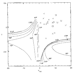
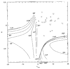
Figure 4: Dependence of the polarization $\Pi$ on $\Omega$ (left panel), on $v_{\rm vis}$ (middle panel) for $\zeta=2.1$ and for $\zeta=3$ (right panel). The emitting particles are concentrated close to the Alfvén resonant surface. Here $B_{\phi}=+\Omega^{F}rB_{z}/c$, fundamental eigenmode with $m=1$. Notations are the same as in Fig. 2. In the left panel solid curves are for $\zeta=2.1$, dashed curves are for $\zeta=3.$

As in Sect. 2 we take $B_{z}=\mbox{constant}$, $B_{\phi}=\pm\Omega^{F}rB_{z}/c$, and take the dependence $\Omega^{F}(r)$ given by expression (18).

The results for uniform particle distribution do not match the observations. Taking into account the presence of the electric field and Doppler boosting changes the polarization of the synchrotron emission essentially. The apparent direction of the magnetic field, as it is usually derived from polarization measurements (just perpendicular to the electric vector in the polarized component of the radiation), is now transversal to the jet axis only for small angle $\theta$ and large $\Omega$. For most inclination angles $\theta$ and angular velocities $\Omega$ the apparent magnetic field is longitudinal (Fig. 4). One can also see from Fig. 4, where we plot $\Pi$ versus $v_{\rm vis}$ for $B_{\phi}=+\Omega^{F}rB_{z}/c$ and for the particles concentrated near Alfvén resonance surface, that our simulation does not match the observational data from Table 1. However, for $B_{\phi}=-\Omega^{F}rB_{z}/c$ we are able to reproduce the observations well enough, if the particles are distributed close to the Alfvén surface and $m=1$ or $m=-1$. In both cases, with and without considering the Doppler boosting effect and the electric field, $\Pi$ is not changed when one changes the sign of $\Omega$, but $\Pi$ is changed when one puts $B_{\phi}=-\Omega^{F}r/cB_{z}$ instead of $B_{\phi}=\Omega^{F}r/cB_{z}$. Let us list all transformations which do not change the equations for the radial displacement $\xi_{r}$ in the perturbations (Istomin & Pariev 1996) or lead to complex conjugated equations for $\xi_{r}^{\star}$:

1. $\omega\to-\omega^{\star}$, $\,k\to-k$, $\,\Omega\to-\Omega$;

2. $\omega\to-\omega^{\star}$, $\,k\to-k$, $\,m\to-m$;

3. $\Omega\to-\Omega$, $\,m\to-m$;

4. $k\to-k$, $\,B_{\phi}=+\Omega^{F}rB_{z}/c\,\to\,B_{\phi}=-\Omega^{F}rB_{z}/c$;

5. $B_{z}\to-B_{z}$.

So, if the eigenvalue stability problem for the radial displacement has one set of parameters listed above as a solution, then the parameters transformed according to the rules 1-5 above will also be a solution of the eigenvalue problem for the radial displacement for the same $\xi_{r}$ or for $\xi_{r}^{\star}$. Therefore, $k_{\rm min}$ and $\omega_{\rm min}$ can be transformed according to the rules 1-5 above and the transformed $k_{\rm min}$ and $\omega_{\rm min}$ will also correspond to the “standing wave” wavenumber and frequency. The value of $r_{A}$ is also not changed under transformation of the parameters listed above. The degree of polarization $\Pi$ is neither influenced by changing the sign of $B_{z}$ nor by changing sign of $\Omega$. The crucial fact is that a sign change in the relation $B_{\phi}=\pm\Omega^{F}rB_{z}/c$ leads to a sign change of $v_{\rm phas}=\omega_{\rm min}/k_{\rm min}$, whilst all other four transformations listed above change neither $\Pi$ nor $v_{\rm phas}$. Therefore, for the purpose of finding the correlation between $\Pi$ and $v_{\rm vis}$, which can be verified observationally, all different cases are reduced to considering two signs in the relation $B_{\phi}=\pm\Omega^{F}rB_{z}/c$, but we can limit ourself only to the consideration of $B_{z}>0$, $m>0$ and all $\Omega$ for which $r_{A}$ is located inside the jet. Using formulae (23)–(27) and expressions (6) for $u_{z}$ and $u_{\phi}$ one can check that the Stokes parameters remain unchanged when one changes the sign of $B_{\phi}$ and replaces angle $\theta$ by $\pi-\theta$. Also, a simultaneous sign change of $v_{\rm phas}$ and change of $\theta$ to $\pi-\theta$ leads to $v_{\rm vis}$ being transformed into $-v_{\rm vis}$. Therefore, the dependence of $\Pi$ on $v_{\rm vis}$ in the case $B_{\phi}=-\Omega^{F}rB_{z}/c$ can be obtained from the same dependence in the case $B_{\phi}=+\Omega^{F}rB_{z}/c$ by reversing the sign of $v_{\rm vis}\to-v_{\rm vis}$ and relabelling each curve from $\theta$ to $\pi-\theta$.

We plotted the degree of linear polarization $\Pi$ versus $v_{\rm vis}$ for $m=1$ in Figs. 4 and 5 for $B_{\phi}=+\Omega^{F}rB_{z}/c$ and $B_{\phi}=-\Omega^{F}rB_{z}/c$ correspondingly. The Alfvén resonance exists for $0.7<\Omega<4.9$. Therefore, the value of $\Omega$ belongs to this interval along the curves in Figs. 4 and 5.

We see that the curves in Fig. 4 do not match the observational data for knots in jets, while those in Fig. 5 do. The dependence on the power-law index $\zeta$ of emitting particles is weak. Our choice of $\zeta=2.1$ and $\zeta=3$ is motivated by the maximum and minimum values of $\zeta$ obtained in the process of the formation of the spectrum of the particles accelerated near the Alfvén resonance surface (Beresnyak et al. 2002).

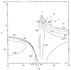
Figure 5: The dependence of polarization $\Pi$ on $\Omega$ (left panel), on $v_{\rm vis}$ for $\zeta=2.1$ (middle panel) and for $\zeta=3$ (right panel). Emitting particles are concentrated close to the Alfvén resonant surface. $B_{\phi}=-\Omega^{F}rB_{z}/c$, fundamental eigenmode with $m=1$. Notations are the same as in Fig. 2. In the left panel solid curves are for $\zeta=2.1$, dashed curves are for $\zeta=3.$

We can suggest the following explanation of the fact that knots are observed more often in jets with $B_{\phi}=-\Omega^{F}rB_{z}/c$ than in jets having the opposite winding of the magnetic field. If we look at the models of the formation of magnetically driven jets from accretion discs (see, e.g. Pelletier & Pudritz 1992) we find that the magnetic field lines are always bent in the direction opposite to the direction of disc rotation as soon as the velocity of the outflow is directed outwards from the disc plane. This means that in the jet approaching the observer $B_{\phi}=-\Omega^{F}rB_{z}/c$, whilst in the jet receding from the observer $B_{\phi}=+\Omega^{F}rB_{z}/c$. Disturbances propagating along the approaching jet should be brighter than those in the counter-jet due to the Doppler boosting effect. Therefore, we will observe knots in parts of jets having $B_{\phi}=-\Omega^{F}rB_{z}/c$ more often than in those parts where $B_{\phi}=+\Omega^{F}rB_{z}/c$. This can explain the fact that the number of sources having $\Pi>0$ is somewhat larger than the number of sources having $\Pi<0$ despite the fact that for most of the values of the parameters calculations give a longitudinal polarization $\Pi<0$. We see from Fig. 5 that our model curves fit the data for BL Lac objects better than those for quasars. On the other hand, the polarization measurements for the quasars are quite different at different frequencies and such differences are larger than the variations of the polarization measurements for the BL Lac objects. In the frame of our model, jets in quasars tend to have higher values of $\Omega^{F}$ than do jets in BL Lac objects. It is remarkable that in quasars knots in jets also have faster apparent motions than in BL Lac objects.

4 Summary

We calculate the linear polarization of the synchrotron radiation produced by fast particles in non-uniformly moving and differentially rotating relativistic flow such as jet flows in AGNs. The magnetic field in the jet has axial and toroidal components. The distribution of the fast particles is taken to be isotropic in the reference frame comoving with the flow. We perform integration of Stokes parameters $I$, $U$, $Q$ along the line of sight passing through the jet with all relativistic effects fully taken into account. We consider two possibilities for the spatial density of the fast particles: 1) ultra-relativistic particles distributed uniformly across the jet, 2) ultra-relativistic particles concentrated close to the Alfvén resonance surface. The latter distribution follows from our acceleration theory and we compare it with the former which might be produced by other acceleration processes. We assume a uniform axial magnetic field in the jet, so the equilibrium configuration of the jet depends only on the radial profile of the angular rotational velocity $\Omega^{F}(r)$ of the magnetic field lines. We take the profile of the angular rotational velocity to be a plausible monotonic function of radius, $\displaystyle\Omega^{F}=\Omega\frac{c}{R}\left(1-\left(\frac{r}{R}\right)^{2}\right)$, and investigate the dependence of polarization on the magnitude of the angular velocity $\Omega$. In our computations we also specify a component of the velocity parallel to the magnetic field lines such that the kinetic energy associated with the flow is minimized. The actual velocity is determined by the process of jet formation, which is poorly understood now; still such minimal velocity is physically favoured (Frolov & Novikov 1998). We calculate the degree of linear polarization and orientation of the electric vector with respect to the jet axis for the emission integrated over the jet cross section, taking into account the relativistic bulk spiral flow of plasma in the jet. This flow leads to the presence of an electric field comparable in magnitude with the magnetic field, causes a Doppler boost of the intensity of the synchrotron radiation, and a swing of the polarization position angle. We want to stress that the last effect, which was first pointed out in 1979 by Blandford & Königl for the simpler case of a uniform magnetic field parallel to the jet axis, substantially modifies the resulting degree of linear polarization from the whole jet. However, because of the axial symmetry of the problem, only two orientations of polarization position angles are possible: parallel or perpendicular with respect to the jet axis. Observations of polarization of VLBI scale jets in BL Lac objects on centimetre wavelengths (Gabuzda et al., 2000) show a bimodal distribution of the position angles: most of the knots in BL Lac objects have polarization either parallel to the jet axis or perpendicular to it. Similar observations of quasars (Lister 2001) on millimetre wavelengths indicate a unimodal distribution of the position angles: most of the knots in the observed quasars have the electric vector of polarized emission oriented along the jet axis. In our present calculations the polarization does not depend on frequency since we have assumed a power-law distribution over the whole range of energies of the particles. Different slopes of the energy spectrum of the particles at different energies can result in a dependence of the degree of polarization and of the position angle on the frequency. This may account for the differences in polarizations at different frequencies observed in quasars. At present, we can only suggest that jets in quasars tend to have larger $\Omega^{F}$ and a larger ratio of toroidal to poloidal magnetic field than do jets in BL Lac objects. This can account for the electric field vector in quasars being predominantly parallel to the jet axis.

We also calculated the velocities of crests of standing eigenmodes and compared them with the observed proper motions of bright VLBI knots in jets. We were able to match the observational data only for the case when the emitting particles are concentrated close to the Alfvén resonance surface and the magnetic field lines are twisted in the direction opposite to the direction of rotation $\Omega^{F}$. The last fact can be understood by a selection effect due to the Doppler boosting which makes jets approaching the observer more favourable to observe than receding jets. Comparing calculations with observations we can estimate the angular rotational velocity of the jets. The trend is that $\Omega^{F}$ in BL Lac objects is intrinsically smaller than in quasars. More detailed calculations considering different possibilities for the $\Omega^{F}(r)$ profile are postponed to another work. There are some discrepancies between our calculations and the observation points (see Fig. 5). It is possible that the radial profile of $\Omega^{F}(r)$ needs to be tuned to provide better agreement. At present it is difficult to suggest a unique test, which would make it possible to distinguish between electromagnetic and shock mechanisms for the origin of knots in jets. Future high-resolution and high-dynamic-range observations could provide detailed images of the spatial structure of knots and surrounding jets, and provide the answer.

References

Attridge J.M., Roberts D.H., & Wardle J.F.C., 1999, ApJ, 518, L87

Begelman M.C., Blandford R.D., & Rees M.J., 1984, Rev. Mod. Phys., 56, 255

Beresnyak A.R., Istomin Ya.N., & Pariev V.I., 2003, A&A, accepted

Blackman E.G., 1996, ApJ, 456, L87

Blandford R.D., & Königl A., 1979, ApJ, 232, 34

Blandford R.D., & Eichler D., 1987, Physics Reports, 154, 1

Cocke W.J., & Holm D.A., 1972, Nature Phys. Sci., 240, 161

Frolov V.P., & Novikov I.D., 1998, Black hole physics: basic concepts and new developments. Kluwer Academic, Dordrecht

Gabuzda D.C., & Cawthorne T.V., 1993, in Davis R.J., Booth R.S., eds, Subarcsecond Radio Astronomy. Cambridge Univ. Press, Cambridge, p.211

Gabuzda D.C., Mullan C.M., Cawthorne T.V., Wardle J.F.C., & Roberts D.H., 1994, ApJ, 435, 140

Gabuzda D.C., 1999a, New Astronomy Reviews, 43, 691

Gabuzda D.C., 1999b, in Ostrowski M., Schlickeiser R., eds, Plasma Turbulence and Energetic Particles in Astrophysics. Uniwersytet Jagiellonski, Cracow, 1999, p.301

Gabuzda D.C., 2000, in Conway J.E., Polatidis A.G., Booth R.S., Pihlström Y.M., eds, EVN Symposium 2000, Proceedings of the 5th European VLBI Network Symposium. Onsala Space Observatory, Onsala, p.53

Gabuzda D.C., Pushkarev A.B., & Cawthorne T.V., 2000, MNRAS, 319, 1109

Gabuzda D.C., Pushkarev A.B., & Garnich N.N., 2001, MNRAS, 327, 1

Ginzburg V.L., 1989, Applications of Electrodynamics in Theoretical Physics and Astrophysics. Gordon and Breach Science Publishers, New York, p.65

Hirotani K., Iguchi S., Kimura M., & Wajima K., 1999, PASJ, 51, 263

Hirotani K., Iguchi S., Kimura M., & Wajima K., 2000, ApJ, 545, 100

Hutchison J.M., Cawthorne T.V., & Gabuzda D.C., 2001, MNRAS, 321, 525

Istomin Ya.N., & Pariev V.I., 1994, MNRAS, 267, 629

Istomin Ya.N., & Pariev V.I., 1996, MNRAS, 281, 1

Königl A., & Choudhuri A.R., 1985, ApJ, 289, 188

Laing K.A., 1981, ApJ, 248, 87

Leppänen K.J., Zensus J.A., & Diamond P.J., 1995, AJ, 110, 2479

Lister M.L., Marscher A.P., & Gear W.K., 1998, ApJ, 504, 702

Lister M.L., 2001, ApJ, 562, 208

Lister M.L., Tingay S.J., & Preston R.A., 2001, ApJ, 554, 964

Manolakou K., Anastasiadis A., & Vlahos L., 1999, A&A, 345, 653

Morrison P., & Sadun A., 1992, MNRAS, 254, 488

Pelletier G., & Pudritz R., 1992, ApJ, 394, 117

Reynolds C.S., Fabian A.C., Celotti A., & Rees M.J., 1996, MNRAS, 283, 873.

Romanova M.M., & Lovelace R.V.E., 1992, A&A, 262, 26

Röser H.-J., & Meisenheimer K., 1991, A&A, 252, 458

Sazonov, V.N., 1969, AZh, 46, 502

Sikora M., & Madejski G., 2000, ApJ, 534, 109

Scheuer P.A.G., 1984, Adv. Space Res., 4, 337

Wardle J.F.C., Homan D.C., Ojha R., & Roberts D.H., 1998, Nature, 395, 457

Zhelezniakov V.V., 1996, Radiation in astrophysical plasmas. Kluwer, Dordrecht