Vacuum polarization and photon mass in inflation

Abstract

We give a pedagogical review of a mechanism through which long wave length photons can become massive during inflation. Our account begins with a discussion of the period of exponentially rapid expansion known as inflation. We next describe how, when the universe is not expanding, quantum fluctuations in charged particle fields cause even empty space to behave as a polarizable medium. This is the routinely observed phenomenon of vacuum polarization. We show that the quantum fluctuations of low mass, scalar fields are enormously amplified during inflation. If one of these fields is charged, the vacuum polarization effect of flat space is strengthened to the point that long wave length photons acquire mass. Our result for this mass is shown to agree with a simple model in which the massive photon electrodynamics of Proca emerges from applying the Hartree approximation to scalar quantum electrodynamics during inflation. A huge photon mass is not measured today because the original phase of inflation ended when the universe was only a tiny fraction of a second old. However, the zero-point energy left over from the epoch of large photon mass may have persisted during the post-inflationary universe as very weak, but cosmological-scale, magnetic fields. It has been suggested that these small seed fields were amplified by a dynamo mechanism to produce the micro-Gauss magnetic fields observed in galaxies and galactic clusters.

I Expanding universe and inflation

The universe is expanding, but with a rate so tiny that it can only be seen by spectroscopic analysis of stars in distant galaxies. Suppose the light from such a star contains a distinctive absorption line measured at the wave length $\lambda$. If the same line occurs at wave length $\lambda_{E}$ on Earth, we say the star’s redshift is,

$$z=\frac{\lambda}{\lambda_{E}}-1\,.$$ (1)

One can also measure the star’s flux ${\cal F}$. If we understand the star enough to know it should emit radiation at luminosity ${\cal L}$, we can infer its luminosity distance $d_{L}$, which is the star’s distance in Euclidean geometry,

$${\cal F}=\frac{\cal L}{4\pi d_{L}^{2}}\quad\Longrightarrow\quad d_{L}=\sqrt{\frac{\cal L}{4\pi{\cal F}}}\,.$$ (2)

Astronomers measure the expansion of the universe by plotting $z$ versus $d_{L}$ for many stars.

Stars throughout the universe move with respect to their local environments at typical velocities of about $10^{-3}$ the speed of light $c$. This motion gives rise to a special relativistic Doppler shift of $\Delta z\sim\pm 10^{-3}$. If spacetime was not expanding, this shift would be the only source of nonzero $z$, and averaging over many stars at the same luminosity distance would give zero redshift. That is just what happens for stars within our galaxy. However, the luminosity distances of stars in distant galaxies are observed to grow approximately linearly with their redshifts,

$$c^{-1}H_{0}d_{L}=z+\frac{1}{2}(1-q_{0})z^{2}+O(z^{3})\,.$$ (3)

Equation (3) means that more and more distant objects seem to recede from us with greater and greater speed. A common analogy is to the way fixed spots move apart on the surface of a balloon that is being blown up.

The constant, $H_{0}\simeq 2.3\times 10^{-18}~{}{\rm Hz}$, is called the Hubble parameter. (When expressed in units used by astronomers, $H_{0}\simeq 71$ km/s/Mpc, where 1 Mpc corresponds to the distance light traverses in about 3.26 million years.) Its name honors Edwin Hubble, who established the (nearly) linear relation Hubble:1929 in 1929 based on his observations, and on earlier work of Slipher and Wirtz Wirtz:1922+1924 . The other constant in Eq. (3) is known as the deceleration parameter, $q_{0}$. Observations of Type Ia supernovae (whose luminosities can be precisely inferred) up to the enormous redshift of 1.7 indicate $q_{0}\simeq-0.6$ Perlmutter-etal:1998 ; Riess-etal:1998 .

The geometry of spacetime is described by a symmetric tensor field $g_{\mu\nu}(x)$ known as the metric. It is used to translate the coordinate labels of points $x^{\mu}=(ct,\vec{x})$ into physical distances and angles. For example, the square of the distance between $x^{\mu}$ and an infinitesimally close point $x^{\mu}+dx^{\mu}$ is known as the invariant interval,

$$ds^{2}\equiv g_{\mu\nu}(x)dx^{\mu}dx^{\nu}\,.$$ (4)

Note that we employ the Einstein summation convention in which repeated indices are summed over $0,1,2,3$.

The transition from nearby stars, whose redshifts are dominated by local motions, to more distant stars which obey Eq. (3), is known as entering the Hubble flow. It is typical in cosmology to ignore local features and model a simplified universe that has only the overall expansion effect. Such a universe does not change in moving between spatial points at the same time, nor are there any special directions. The first property is known as homogeneity; the second is isotropy.

With a simplifying assumption — about which more later — the invariant interval of a homogeneous and isotropic universe can be written as

$$ds_{\rm HI}^{2}=-c^{2}dt^{2}+a^{2}(t)d\vec{x}\cdot d\vec{x}\,.$$ (5)

From this relation we see that $t$ measures physical time the same way as in the Minkowski geometry. However, the spatial 3-vector $\vec{x}$ must be multiplied by $a(t)$ to give physical distances. For this reason $a(t)$ is known as the scale factor. Its time variation gives the instantaneous values of the Hubble and deceleration parameters,

$$H(t)\equiv\frac{\dot{a}}{a},\qquad q(t)\equiv-\frac{a\ddot{a}}{\dot{a}^{2}}=-1-\frac{\dot{H}}{H^{2}}\,.$$ (6)

The 0 subscripts on $H_{0}$ and $q_{0}$ in Eq. (3) and the subsequent discussion indicate the current values of these parameters.

Homogeneity and isotropy restrict the stress-energy tensor to only an energy density $\rho(t)$ and a pressure $p(t)$,

$$T_{00}=-\rho(t)g_{00},\qquad T_{0i}=0,\qquad T_{ij}=p(t)g_{ij},$$ (7)

where $i$ and $j$ are spatial indices. In this geometry Einstein’s equations take the form,

$$3H^{2} = 8\pi Gc^{-2}\rho\,,$$ (8)

$$-2\dot{H}-3H^{2} = 8\pi Gc^{-2}p\,,$$ (9)

where $G$ is Newton’s constant. The current energy density is,

$$\rho_{0}=\frac{3c^{2}H_{0}^{2}}{8\pi G}\simeq 8.5\times 10^{-10}~{}{\rm J/m}^{3}\,,$$ (10)

equivalent to about 5.7 Hydrogen atoms per cubic meter. If we solve for the instantaneous deceleration parameter,

$$q=\frac{1}{2}+\frac{3p}{2\rho}\,,$$ (11)

we find that $p_{0}\simeq-0.7\rho_{0}$ Bennett:wmap2003 ; Spergel:wmap2003 .

By differentiating Eq. (8) and then adding $3H$ times Eq. (8) plus Eq. (9), we derive a relation between the energy density and pressure known as stress-energy conservation,

$$\dot{\rho}=-3H(\rho+p)\,.$$ (12)

If we also assume a constant equation of state, $w\equiv p(t)/\rho(t)$, Eq. (12) can be used to express the energy density in terms of the scale factor,

$$\rho(t)=\rho_{1}\Bigl{(}\frac{a(t)}{a_{1}}\Bigr{)}^{-3(1+w)}\,.$$ (13)

The substitution of Eq. (13) in Eq. (8) gives an equation whose solution is,

$$a(t)=a_{1}\Bigl{[}1+\frac{3}{2}(1+w)H_{1}(t-t_{1})\Bigr{]}^{\frac{2}{3(1+w)}}\,.$$ (14)

The cases of $w=+\frac{1}{3}$, 0,$-\frac{1}{3}$, and $-1$ correspond to radiation, non-relativistic matter, spatial curvature, and vacuum energy, respectively. (We do not discuss here scalar field matter RatraPeebles:1987 , usually referred to as quintessence CaldwellDaveSteinhardt:1997 , with nonconstant $w$.) The cosmology for each pure type of stress-energy can be read off from Eqs. (13) and (14),

Radiation $$\Longrightarrow \rho\propto a^{-4},\quad a(t)\propto(H_{1}t)^{\frac{1}{2}},$$

Non-Relativistic Matter $$\Longrightarrow \rho\propto a^{-3},\quad a(t)\propto(H_{1}t)^{\frac{2}{3}},$$

Curvature $$\Longrightarrow \rho\propto a^{-2},\quad a(t)\propto H_{1}t,$$

Vacuum Energy $$\Longrightarrow \rho\propto 1,\hskip 24.0pta(t)\propto e^{H_{1}t}.$$

The actual universe seems to be composed of at least three of the pure types, so the scale factor does not have a simple time dependence. However, as long as each type is separately conserved, we can use Eq. (13) to conclude that

$$\rho(t)=\frac{\rho_{\rm rad}}{a^{4}(t)}+\frac{\rho_{\rm mat}}{a^{3}(t)}+\frac{\rho_{\rm cur}}{a^{2}(t)}+\rho_{\rm vac}\,.$$ (19)

As the universe expands, the relative importance of the four types changes. Whenever a single type predominates, we can infer $a(t)$ from Eq. (14). This different dependence is one reason it makes sense to think of an early universe dominated by radiation, Eq. (LABEL:raddom), evolving to a universe dominated by non-relativistic matter, Eq. (LABEL:matdom). It is also how we can understand that the current universe seems to be making the transition to domination by vacuum energy, Eq. (LABEL:dS).

Under certain conditions there can be significant energy flows between three of the pure types of stress-energy. For example, as the early universe cooled, massive particles changed from behaving like radiation to behaving like non-relativistic matter. This change would increase $\rho_{\rm mat}$ and decrease $\rho_{\rm rad}$ in Eq. (19). The parameter that cannot change is that of the spatial curvature, $\rho_{\rm cur}$. Strictly speaking, we should not regard spatial curvature as a type of stress-energy, but rather as an additional parameter in the homogeneous and isotropic metric Eq. (5). We have avoided this complication because the extra terms it gives in the Einstein equations (8)–(9) can be subsumed into the energy density and pressure, as we have done, and because the measured value of $\rho_{\rm cur}/a_{0}^{2}$ is consistent with zero Bennett:wmap2003 ; Spergel:wmap2003 .

The cosmology in which a radiation dominated universe evolves to matter domination is a feature of what is known as the Big Bang scenario. Although strongly supported by observation, the composition of $\rho$ at the start of radiation domination ($t=t_{r}$ and $a=a_{r}$) does not seem natural,

$$\rho_{\rm rad}a_{r}^{-4}\gg\rho_{\rm vac}\gg\rho_{\rm cur}a_{r}^{-2}\,.$$ (20)

It might be expected instead that each of the three terms was comparable, in which case the universe would quickly become dominated by vacuum energy. There is no accepted explanation for the first inequality in Eq. (20) or for the seeming coincidence that $\rho_{\rm mat}a_{0}^{-3}\sim\rho_{\rm vac}$. However, the second inequality in Eq. (20) finds a natural explanation in the context of inflation.

In 1980 Alan Guth Guth:1980 suggested that the Big Bang scenario was preceded by a period of vacuum energy domination, or inflation, following which the vacuum energy changed almost completely into radiation. (Cosmologies that include a period of vacuum energy domination were independently considered by Starobinsky Starobinsky:1980 , Sato Sato:1981 , and by Kazanas Kazanas:1980 .) Suppose that all types of stress-energy are equally represented at some very early time. We see from Eq. (19) that the total energy density rapidly becomes dominated by vacuum energy, following which the scale factor grows exponentially with a constant Hubble parameter, $H_{I}$.

The duration of inflation in units of $1/H_{I}$ is known as the number of inflationary e-foldings $N_{I}$. Viable models must have $N_{I}\mathrel{\raise 1.29167pt\hbox{$>$\kern-7.5pt\lower 4.30554pt\hbox{$\sim$}}}50$, and much larger values are common. If $\rho_{\rm cur}/a^{2}_{I}\sim\rho_{\rm vac}$ at the start of inflation, Eq. (19) shows that the curvature is negligible at the end,

$$\frac{\rho_{\rm cur}/a_{r}^{2}}{\rho_{\rm vac}}\sim\Bigl{(}\frac{a_{I}}{a_{r}}\Bigr{)}^{2}=e^{-2N_{I}}\mathrel{\raise 1.29167pt\hbox{$<$\kern-7.5pt\lower 4.30554pt\hbox{$\sim$}}}10^{-44}\,.$$ (21)

Inflation makes the other types of stress-energy even smaller, but there are mechanisms through which vacuum energy can be converted into radiation. This process, which we will not discuss, is known as reheating.

Inflation also explains how the large scale universe became so nearly homogeneous and isotropic. This explanation is crucial because gravity makes even tiny inhomogeneities grow, and the process has had 13.7 billion years to operate. It is believed that the galaxies of today’s universe had their origins in quantum fluctuations of magnitude ${\Delta\rho}/\rho\simeq 10^{-5}$, which occurred during the last 60 e-foldings of inflation. The imprint of these fluctuations in the cosmic microwave background has recently been imaged with unprecedented accuracy by the WMAP satellite Bennett:wmap2003 ; Spergel:wmap2003 .

The fact that WMAP did not see the imprint of quantum fluctuations of the metric field sets an upper limit of $H_{I}\mathrel{\raise 1.29167pt\hbox{$<$\kern-7.5pt\lower 4.30554pt\hbox{$\sim$}}}3.4\times 10^{38}$ Hz. No one knows what caused inflation, but a common assumption is that it occurred at the grand unified energy scale $E_{\rm GUT}\simeq 10^{16}\,{\rm GeV}\simeq 10^{6}$ J at which electromagnetic, weak, and strong interactions attain equal strength. From Eq. (8) this implies,

$$H_{I}=\Bigl{(}\frac{8\pi G}{3c^{2}}\frac{E^{4}_{\rm GUT}}{(\hbar c)^{3}}\Bigr{)}^{\frac{1}{2}}\simeq 10^{37}\,{\rm Hz}\,,$$ (22)

where we used $\rho_{\rm GUT}=E_{\rm GUT}/V_{\rm GUT}$, $V_{\rm GUT}=(\hbar c/E_{\rm GUT})^{3}$ defines the GUT energy scale volume, and $\hbar\simeq 1.05\times 10^{-34}$ J s is the reduced Planck constant.

II Vacuum polarization in flat space

Flat space corresponds to $a(t)=1$ in Eq. (5),

$$ds^{2}_{\rm flat}=\eta_{\mu\nu}dx^{\mu}dx^{\nu}=-c^{2}dt^{2}+d\vec{x}\cdot d\vec{x}\,.$$ (23)

Note that the zero component of a spacetime point $x^{\mu}=(ct,\vec{x})$ is $x^{0}=ct$, so all components of $\partial_{\mu}\equiv\partial/\partial x^{\mu}$ have the dimension of inverse length. Repeated Greek indices are summed over $0,1,2,3$ — for example, $\partial^{2}\equiv\partial_{\mu}\partial^{\mu}$ — whereas repeated Latin indices are summed over $1,2,3$ — for example, $\nabla^{2}\equiv\partial_{i}\partial_{i}$. A dot denotes contraction over the appropriate index set, for example, $k\cdot x\equiv k_{\mu}x^{\mu}$ and $\vec{k}\cdot\vec{x}\equiv k_{i}x_{i}$.

To make Lorentz invariance manifest, we employ the Heaviside-Lorentz system of units in which Maxwell’s equations take the form,

$$\vec{\nabla}\cdot\vec{E}=\rho, \vec{\nabla}\times\vec{B}-\partial_{0}\vec{E}=c^{-1}\vec{J}\,,$$ (24)

$$\vec{\nabla}\cdot\vec{B}=0, \vec{\nabla}\times\vec{E}+\partial_{0}\vec{B}=0\,.$$ (25)

Here $\vec{E}(t,\vec{x})$ and $\vec{B}(t,\vec{x})$ denote the electric and magnetic fields, and the charge and current densities are $\rho(t,\vec{x})$ (for this section only) and $\vec{J}(t,\vec{x})$. The more familiar MKSA formulation of electrodynamics follows from the substitutions,

$$\vec{E}\rightarrow\epsilon_{0}\vec{E}_{\scriptscriptstyle\rm MKSA},\;\vec{B}\rightarrow\sqrt{\frac{\epsilon_{0}}{\mu_{0}}}\vec{B}_{\scriptscriptstyle\rm MKSA},\ {\rm and}\;c\rightarrow\frac{1}{\sqrt{\epsilon_{0}\mu_{0}}}\,,$$ (26)

where $\epsilon_{0}$ and $\mu_{0}$ are, respectively, the electric permittivity and the magnetic permeability of free space.

It is well known that Eq. (25) can be enforced by representing the fields using a vector potential $A_{\mu}=(A_{0},A_{i})$,

$$E^{i}=\partial_{0}A_{i}-\partial_{i}A_{0},\qquad B^{i}=-\epsilon^{ijk}\partial_{j}A_{k}\,.$$ (27)

Equations (24) combine to the relativistic form,

$$\partial_{\nu}F^{\nu\mu}=c^{-1}J^{\mu}\,,$$ (28)

using the field strength tensor $F_{\mu\nu}\equiv\partial_{\mu}A_{\nu}-\partial_{\nu}A_{\mu}$ and the current 4-vector $J^{\mu}\equiv(c\rho,\vec{J})$.

Material media such as air and glass consist of an enormous number of atoms with negatively charged electrons bound to positively charged nuclei. On macroscopic scales such a medium appears neutral and free of currents, but the application of external fields can distort the bound charges to induce a density of atomic electric dipole moments known as the polarization $\vec{P}(t,\vec{x})$, which we illustrate on a gas of polarized atoms in figure 1. Averaging the actual charge density to remove its violent fluctuations on the atomic scale leaves whatever charges are free, minus the gradient of $\vec{P}$,

$$\langle\rho\rangle=\rho_{\rm free}-\vec{\nabla}\cdot\vec{P}\,.$$ (29)

The medium’s density of atomic magnetic dipole moments is known as its magnetization $\vec{M}(t,\vec{x})$. A similar averaging of the current density gives,

$$\langle\vec{J}\rangle=\vec{J}_{\rm free}+c\partial_{0}\vec{P}+c\vec{\nabla}\times\vec{M}\,.$$ (30)

Moving the polarization and magnetization terms to the left-side of Eq. (24) leads to the macroscopic Maxwell equations,

$$\vec{\nabla}\cdot\vec{D} = \rho_{\rm free}$$

$$\vec{\nabla}\times\vec{H}-\partial_{0}\vec{D} = c^{-1}\vec{J}_{\rm free}\,,$$ (31)

where $\vec{D}\equiv\vec{E}+\vec{P}$ and $\vec{H}\equiv\vec{B}-\vec{M}$.

Linear, isotropic media with no frequency or wave number dependence are characterized by,

$$\vec{P}=\chi_{e}\vec{E},\qquad\vec{M}=\frac{\chi_{m}}{1+\chi_{m}}\vec{B}\,.$$ (32)

The dimensionless parameters $\chi_{e}$ and $\chi_{m}$ are known as the electric and magnetic susceptibilities. We would like to express Eq. (31) as a single tensor equation like Eq. (28). For the case of constant susceptibilities the result is simple:

$$\partial_{\nu}F^{\nu\mu}+\Pi^{\mu\nu}A_{\nu}=c^{-1}J^{\mu}_{\rm free}\,.$$ (33)

where $\Pi^{\mu\nu}$ is the following tensor differential operator,

$$\Pi^{\mu\nu} \equiv \chi_{e}\Bigl{(}\eta^{\mu\nu}\partial^{2}-\partial^{\mu}\partial^{\nu}\Bigr{)}$$ (34)

$$- \Bigl{(}\chi_{e}+\frac{\chi_{m}}{1+\chi_{m}}\Bigr{)}\eta^{\mu i}\eta^{\nu j}\Bigl{(}\delta_{ij}\nabla^{2}-\partial_{i}\partial_{j}\Bigr{)}\,.$$

The polarization tensor encapsulates the medium’s effect on electromagnetic forces and on propagating electromagnetic fields. It is useful to recall the familiar formulae for the relative permittivity and permeability and for the index of refraction,

$$\epsilon=1+\chi_{e},\qquad\mu=1+\chi_{m},\qquad n=(\epsilon\mu)^{\frac{1}{2}}\,.$$ (35)

The susceptibility $\chi_{e}$ in Eq. (34) gives the medium’s corrections to the electric response to a static distribution of charge. Positive $\chi_{e}$ means that the medium’s dipoles line up to weaken an applied electric field by a factor of $1/\epsilon$. This effect is known as charge screening. The other term in Eq. (34) can be understood by recasting its integrand,

$$\chi_{e}+\frac{\chi_{m}}{1+\chi_{m}}=\epsilon-\frac{1}{\mu}=\bigl{(}n^{2}-1\bigr{)}\frac{1}{\mu}\equiv\delta n^{2}\,.$$ (36)

Together with $\epsilon$, $\delta n^{2}$ gives the medium’s corrections to the magnetic response to currents. It also governs the speed $c/n$ at which electromagnetic waves propagate, such that, whenever $\delta n^{2}\neq 0$ ($n\neq 1)$, the speed of light differs from that in the (Minkowski) vacuum.

   

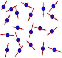
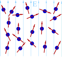
Figure 1: A gas of polarized atoms. In the absence of an external electric field the dipoles orient randomly (FIG. 1a). When an external field $\vec{E}$ is applied, the dipoles tend to line up with it (FIG. 1b). This alignment produces a net polarization, $\vec{P}=\chi_{e}\vec{E}$, which weakens the electric force by $1/(1+\chi_{e})$. There is a similar effect in vacuum due to oppositely charged pairs of evanescent, virtual particles.

The susceptibilities of real media typically vary according to the frequency and sometimes even the wave number of the external field Jackson:III . One reason for this variation is that the bound charges in a medium cannot respond infinitely quickly to changes in the applied electromagnetic fields, so the polarization must be attenuated at high frequencies. There also can be resonant effects when the applied electromagnetic fields perturb systems of bound charges near their natural vibrational frequencies.

Whatever the reason for it, we should understand that frequency and wave number dependence invalidates the local constitutive relations (32) and hence, the tensor equation (33) we have derived from them. Maxwell’s equations in media (31) are still correct, but the relations between the polarization and magnetization and the applied fields are only multiplicative in frequency-wave number space. To calculate $\vec{P}(t,\vec{x})$ and $\vec{M}(t,\vec{x})$, we first decompose the electric and magnetic fields into their amplitudes for each wave 4-vector $k^{\mu}\equiv(\omega/c,\vec{k})$. This decomposition is equivalent to taking the Fourier transform, and we denote the result with a tilde as follows,

$$\widetilde{E}^{i}(\omega,\vec{k})\equiv\!\int d^{4}xe^{i\omega t-i\vec{k}\cdot\vec{x}}E^{i}(t,\vec{x})\,.$$ (37)

To get the polarization, we multiply by the $k^{\mu}$ dependent susceptibility and use the Fourier inversion theorem,

$$P^{i}(t,\vec{x})=\!\int\!\frac{d^{4}k}{(2\pi)^{4}}e^{ik\cdot x}\chi_{e}(k)\widetilde{E}^{i}(\omega,\vec{k})\,.$$ (38)

The analogous procedure gives the magnetization.

We have just seen that properly accounting for the $k^{\mu}$ dependence of real media requires us to perform two 4-dimensional integrations: first over spacetime to Fourier transform the fields, and then over $k^{\mu}$. This is tedious and unnecessary. By calculating the Fourier inverse of the susceptibility once and for all,

$$\chi_{e}(x,x^{\prime})\equiv\!\int\!\frac{d^{4}k}{(2\pi)^{4}}\chi_{e}(k)e^{ik\cdot(x-x^{\prime})}\,,$$ (39)

we can reduce the process of dealing with different applied electric fields to a single spacetime integral,

$$P^{i}(t,\vec{x})=\!\int\!d^{4}x^{\prime}\chi_{e}(x,x^{\prime})E^{i}(t^{\prime},\vec{x}^{\prime})\,.$$ (40)

An analogous simplification can be made for the magnetization.

We are now ready to give the generalization of Eq. (33) which applies for the case of $k^{\mu}$ dependent media,

$$\eta^{\mu\nu}\eta^{\rho\sigma}\partial_{\rho}F_{\sigma\nu}(x)\!+\!\!\int\!d^{4}x^{\prime}[\mbox{}^{\mu}\Pi^{\nu}]\!(x,x^{\prime})A_{\nu}(x^{\prime})\!=c^{\!-1}\!J^{\mu}_{\rm free}(x).$$ (41)

The polarization bi-tensor has the general form,

$$[\mbox{}^{\mu}\Pi^{\nu}]\!(x,x^{\prime}) \equiv -[\eta^{\mu\nu}\eta^{\rho\sigma}-\eta^{\mu\rho}\eta^{\sigma\nu}]\partial^{\prime}_{\rho}\partial_{\sigma}\chi_{e}(x,x^{\prime})$$ (42)

$$+ \eta^{\mu i}\eta^{\nu j}[\delta_{ij}\partial^{\prime}_{k}\partial_{k}-\partial^{\prime}_{i}\partial_{j}]\delta n^{2}(x,x^{\prime})\,,\quad$$

where $\partial_{\mu}=\partial/\partial x^{\mu}$, $\partial_{\mu}^{\prime}=\partial/\partial x^{\prime\mu}$ and,

$$\delta n^{2}(x,x^{\prime})=\!\!\int\!\!\frac{d^{4}k}{(2\pi)^{4}}\Bigl{(}\chi_{e}(k)\!+\!\frac{\chi_{m}(k)}{\mu(k)}\Bigr{)}e^{ik\cdot(x-x^{\prime})}\!.$$ (43)

We have actually done a little better than intended. For although Eqs. (39) and (43) apply only to translation invariant and infinite media, Eqs. (41)–(42) give the response from any linear, isotropic medium. For example, we could use this formalism to describe a system in which the local index of refraction varies in space or even in time. Although we shall not consider spatial dependence, this natural way of incorporating time dependence will be quite useful when we consider electrodynamics in an expanding universe.

The designation of $[^{\mu}\Pi^{\nu}](x,x^{\prime})$ as a bi-tensor derives from general relativity in which the index $\mu$ transforms according to the vector space at $x^{\mu}$ and the index $\nu$ according to the vector space at $x^{\prime\mu}$. Note further that $[^{\mu}\Pi^{\nu}]$ is transverse on both indices,

$$\partial_{\mu}[^{\mu}\Pi^{\nu}](x,x^{\prime})=0=\partial_{\nu}^{\prime}[^{\mu}\Pi^{\nu}](x,x^{\prime})\,.$$ (44)

Let us explore the dynamical consequences of an infinite, translational invariant medium for which Eqs. (39) and (43) pertain. In this case we may as well Fourier transform (41) in the Coulomb gauge, $k_{i}\widetilde{A}_{i}(k)=0$. The $\mu=0$ component,

$$-\epsilon(k)\|\vec{k}\|^{2}\widetilde{A}^{0}(k)=c^{-1}\widetilde{J}^{0}(k)\,,$$ (45)

determines the scalar potential from the charge density. As claimed, the medium screens the electric forces by a factor of $1/\epsilon(k)$. The $\mu=i$ equations are more interesting:

$$-\epsilon(k)\Bigl{[}\frac{\|\vec{k}\|^{2}}{n^{2}(k)}-\frac{\omega^{2}}{c^{2}}\Bigr{]}\widetilde{A}^{i}(k)=\frac{1}{c}\Bigl{[}\delta^{ij}-\frac{k^{i}k^{j}}{\|\vec{k}\|^{2}}\Bigr{]}\widetilde{J}^{j}(k)\,.$$ (46)

In addition to the response to a current, the 3-vector potential can also support plane waves that obey the following dispersion relation,

$$\epsilon(k)\Bigl{[}n^{-2}(k)\|\vec{k}\|^{2}-c^{-2}\omega^{2}\Bigr{]}=0\,.$$ (47)

Einstein’s great contribution to quantum theory was the inference (from the photoelectric effect) that light is quantized in discrete photons of energy $E=\hbar\omega$ and 3-momentum $\vec{p}=\hbar\vec{k}$.

When $\epsilon(k)$ is nonsingular, Eq. (47) implies the usual relation, $\omega=(c/n)\|\vec{k}\|$. For this case the energy vanishes as the wave length becomes infinite. However, suppose the medium obeys,

$$\chi_{e}(k)=\frac{m_{\gamma}^{2}c^{2}}{\hbar^{2}k\!\cdot\!k},\qquad n(k)=1\,,$$ (48)

where, as we will see in the following, $m_{\gamma}$ denotes the photon mass. Although the full significance of the singular behavior (48) will become clear later, here we note that it may arise, for example, in the presence of charged particles that are constantly created, and which propagate with the speed of light. From the point of view of the photons, a large number of these particles may lie on its past light cone, at which $k\cdot k=0$, and may thus induce a large (singular) contribution to the susceptibility. The substitution of Eq. (48) in Eq. (47) gives,

$$\epsilon(k)\Bigl{[}n^{-2}(k)\|\vec{k}\|^{2}-\frac{\omega^{2}}{c^{2}}\Bigr{]}=k\!\cdot\!k+\frac{m_{\gamma}^{2}c^{2}}{\hbar^{2}}=0\,.$$ (49)

Such a photon’s energy is that of a massive particle,

$$E=\hbar\omega=\sqrt{\|\vec{p}\|^{2}c^{2}+m_{\gamma}^{2}c^{4}}\,.$$ (50)

We have so far discussed classical media. Quantum field theory predicts that particle-antiparticle pairs are continually being created. They live for a brief period of time and then annihilate one another. The lifetime of such a virtual particle pair is governed by its energy through the energy-time uncertainty principle,

$${\Delta t}{\Delta E}\mathrel{\raise 1.29167pt\hbox{$>$\kern-7.5pt\lower 4.30554pt\hbox{$\sim$}}}\hbar\,,$$ (51)

The meaning of Eq. (51) is that a minimum time ${\Delta t}$ is needed to resolve the energy with accuracy ${\Delta E}$. Suppose each partner of a virtual particle pair has energy $E$. Before they emerged from the vacuum, the energy was zero, whereas it is $2E$ afterward. This is an example of nonconservation of energy! However, Eq. (51) says that the violation is not detectable in a period shorter than $\hbar/2E$, so virtual particles can survive roughly that long.

All types of particles experience virtual particle creation with all possible energies and 3-momenta. One way of understanding the electrostatic force is through the exchange of virtual photons. Because normal photons are massless, they can have arbitrarily small energies and can therefore survive long enough to mediate the force between distant charges. However, the lifetimes of massive particles are extremely short. For example, the minimum energy an electron can have is that of its rest mass, $m_{e}c^{2}\simeq 8.2\times 10^{-14}$ J. From Eq. (51) we see that an electron-positron pair can only live about $\hbar/2m_{e}c^{2}\simeq 6.4\times 10^{-22}$ s. Even moving at nearly the speed of light (which implies higher energy, and hence shorter lifetime), a virtual electron would only cover about $10^{-13}$ m before annihilating, which is a thousand times smaller than the scale upon which the discrete electrons and nuclei are separated in atoms. This explains why macroscopic experiments do not detect virtual electron-positron pairs.

Charged virtual particles behave much like the bound charges of atoms in a polarizable medium. When no external field is present, the positive partner of a virtual pair emerges as often in one direction as any other. However, the application of an electric field makes it preferable for the positive partner to emerge in the direction of the field, while the negative partner emerges in the opposite direction. In this way even empty space can acquire a polarization. The effect is known as vacuum polarization, and it is described with the same Eqs. (41)–(42) which we introduced to quantify the polarization of material media.

Although all charged virtual particles contribute to vacuum polarization, the largest effect comes from the lightest particles because they live the longest. Electrons and positrons are about 200 times lighter than the next lightest charged particles, muons, so almost all vacuum polarization comes from them. By making use of rather sophisticated techniques of quantum electrodynamics, one can show that, at lowest order in $\alpha$, they induce the following electric susceptibility PeskinSchroeder:1995 ,

$$\chi_{e}(k,\Lambda) = 8\pi\alpha\!\int_{0}^{1}dxx(1-x)\!\int^{\Lambda}\!\frac{d^{3}p}{(2\pi)^{3}}$$ (52)

$$\times \Bigl{[}\|\,\vec{p}\,\|^{2}+\Bigl{(}\frac{m_{e}c}{\hbar}\Bigr{)}^{2}+x(1\!-\!x)k\cdot k\Bigr{]}^{-\frac{3}{2}},\quad$$

where $\alpha\equiv e^{2}/4\pi\hbar c\simeq 1/137$ is the fine structure constant. The integral over $\vec{p}$ represents the contribution from an electromagnetic field of wave vector $\vec{k}$ exciting an electron with wave vector $\vec{p}+x\vec{k}$ and a positron with wave vector $-\vec{p}+(1-x)\vec{k}$.

The process described by Eq. (52) conserves 3-momentum ($=\hbar\times{\rm wave\ vector}$), but it need not conserve energy,

$$\hbar ck^{0} \longrightarrow \sqrt{m_{e}^{2}c^{4}+\hbar^{2}c^{2}\|\vec{p}+x\vec{k}\|^{2}}$$ (53)

$$+\;\sqrt{m_{e}^{2}c^{4}+\hbar^{2}c^{2}\|\vec{p}-(1-x)\vec{k}\|^{2}}.$$

The energy of the electron-positron pair can be very much larger than the energy of the initial and final photons, which means the pair can exist only a short time. As one might expect, pairs with very high $\|\vec{p}\|$ do not contribute much susceptibility because they exist too briefly to polarize much. However, there are so many states with large $\|\vec{p}\|$ that their net contribution diverges. That is why we have cut the integral off in Eq. (52) for $\|\vec{p}\|\leq\Lambda$. If we integrate over the momenta, and expand in powers of $1/\Lambda$, we obtain,

$$\chi_{e}(k,\Lambda) = \frac{4\alpha}{\pi}\!\int_{0}^{1}dxx(1-x)\Bigl{[}\ln\Big{(}\frac{2\hbar\Lambda}{m_{e}c}\Big{)}-1$$ (54)

$$- \frac{1}{2}\ln\Bigl{(}1+x(1-x)\frac{\hbar^{2}k\cdot k}{m_{e}^{2}c^{2}}\Bigr{)}+O(1/\Lambda)\Bigr{]}.\qquad$$

We see that the susceptibility diverges logarithmically in the limit that $\Lambda\rightarrow\infty$. This is a classic example of an ultraviolet divergence in quantum field theory. (The adjective ultraviolet is used because the problem originates from high energy — or ultraviolet — pairs.)

The infinite susceptibility is not directly observable because it is a constant, independent of the wave 4-vector $k^{\mu}$ of the applied electrodynamic field. All observable quantities depend as well upon the equally constant, bare charges of particles whose motions reveal the field. For example, consider the force between two particles of charge $e_{\rm bare}$ that are held a fixed distance $r$ from one another. Because the system is constant in time, we have $k^{0}=0$. Because the physical dimension of the system is $r$, the maximum response is for wave vectors of about $\|\vec{k}\|\sim 2\pi/r$. As the separation becomes larger, the significant wave vectors become ever closer to zero. For very large separations the force is therefore $1/r^{2}$ times the quantity, $e^{2}_{\rm bare}/4\pi[1+\chi_{e}(0,\Lambda)]$. The case of large separations (on the scale of $10^{-13}$ m) is one that we can access quite easily, and most everyone who takes introductory physics performs such a measurement. Because the result is finite, it follows that the ratio $e^{2}_{\rm bare}/[1+\chi_{e}(0,\Lambda)]$ must be a finite number that we call $e^{2}$, the square of the measured charge. In other words, the divergence in the unobservable quantity $e^{2}_{\rm bare}$ cancels the divergence in the equally unobservable quantity $\chi_{e}(0,\Lambda)$ so that their ratio agrees with what we measure. To leading order in $\alpha$, the finite $k^{\mu}$ dependent susceptibility, which remains when measured charges are used, is,

$$\chi_{e}(k) = \lim_{\Lambda\rightarrow\infty}\Bigl{\{}\chi_{e}(k,\Lambda)-\chi_{e}(0,\Lambda)\Bigr{\}}$$

$$= -\frac{2\alpha}{\pi}\!\int_{0}^{1}\!dx\,x(1-x)\ln\Bigl{[}1+x(1-x)\frac{\hbar^{2}k\!\cdot\!k}{m_{e}^{2}c^{2}}\Bigr{]}.\quad$$

This discussion illustrates how the process of renormalization works in quantum field theory. We mention it only to explain why the finite remainder Eq. (LABEL:QED4c) can make electromagnetic forces stronger at short distances. Recall that the least energetic electron-positron pairs can only survive long enough to travel about $10^{-13}$ m. More energetic virtual pairs are limited to even shorter distances. This means that charged particles separated by more than about $10^{-13}$ m feel the polarizations contributed by virtual pairs of all 3-momenta. But at separations of less than $10^{-13}$ m, the lower energy virtual pairs leave the electric field between the two charges before fully polarizing. The net effect is less charge screening than at large distances, and hence a relative enhancement of the electromagnetic force at short distances.

This effect is known as running of the force law, and it is seen routinely in precision measurements. In high energy accelerators such as LEP at CERN and SLC at Stanford University, charged particles have been brought as close as $\sim 10^{-18}$ m. The substitution of $k\!\cdot\!k=(2\pi/10^{-18}$ m$)^{2}$ in Eq. (LABEL:QED4c) gives $\chi_{e}\simeq-0.023$, or a 2.3% enhancement of the electromagnetic force.

If the electron mass had been zero, we would see the electromagnetic force law run even at macroscopic distances. In that case the renormalized $e^{2}$ would be $4\pi R^{2}$ times the measured force at some $R$, and this length would enter the formula for $\chi_{e}(k)$,

$$\chi_{e}(k)\Bigl{|}_{m_{e}=0}\longrightarrow-\frac{\alpha}{3\pi}\ln(\mu^{2}k\!\cdot\!k),\quad{\rm where}\quad\mu=\frac{R}{2\pi}.$$ (57)

For $r>R$ we would measure the force to be smaller than $e^{2}/4\pi r^{2}$, whereas it would be greater for $r<R$. The experiment could be done using the apparatus depicted in Fig. 2 WilliamsFallerHill:1971 ; GoldhaberNieto:1971 .

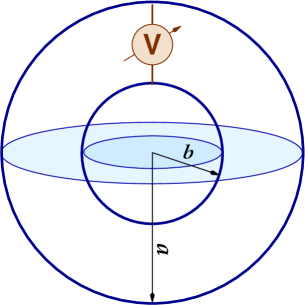
Figure 2: A sketch of the Maxwell-Cavendish experiment. Two metal concentric spheres of radii $a$ and $b$ are first grounded, then the outer sphere is raised to a high potential. If Coulomb’s law were violated, the voltmeter $V$ would show a non-zero voltage.

We have so far discussed only the term $\chi_{e}(x,x^{\prime})$. It turns out that $\delta n^{2}(x,x^{\prime})$ is zero for all relativistic quantum field theories in flat space. This must be so because the tensor coefficient of $\delta n^{2}(x,x^{\prime})$ in Eq. (42) breaks the Lorentz symmetry between space and time. One consequence is that the index of refraction is one, so vacuum polarization does not modify the speed of light. Because the invariant element of an expanding universe Eq. (5) also distinguishes between space and time, we might expect that $\delta n^{2}(x,x^{\prime})\neq 0$ when the Hubble parameter is nonzero, and we will see that this is the case.

Because Eq. (LABEL:QED4c) has no pole at $k\!\cdot\!k=0$, the vacuum polarization from quantum electrodynamics preserves the photon’s zero mass. This turns out to be a slightly mass and dimension-dependent statement. In 1962 Julian Schwinger showed that zero mass electrons in one spatial dimension would induce the following electric susceptibility Schwinger:1962 ,

$$\chi_{e}(k)=\frac{4\alpha}{k\!\cdot\!k}\,.$$ (58)

(In two spacetime dimensions $e^{2}$ has the dimension of ${\rm energy/length}$, which means that $\alpha$ has the dimension of ${\rm length}^{-2}$.) A comparison with Eq. (48) implies a photon mass of $m_{\gamma}=2\sqrt{\alpha}\hbar/c$. We will see later that the expansion of spacetime can also induce a nonzero photon mass.

Electrons and positrons, both of which are spin 1/2 particles, are not the only kinds of charged particles. To obtain the susceptibility contributed by other kinds of spin $\frac{1}{2}$ particles, we simply replace $m_{e}$ in Eq. (LABEL:QED4c) by the appropriate mass. Charged particles with spin zero — which are known as scalars — also entail replacing the factor of $x(1-x)$ which multiplies the logarithm in Eq. (LABEL:QED4c) by $(1-2x)^{2}/8$. The susceptibility of a zero mass scalar would be $\frac{1}{4}$ times that of Eq. (57). It is actually simpler to express the polarization of massless particles in position space by performing the Fourier transform of the electric susceptibility, as indicated in Eq. (39). The result for a massless, charged scalar is ProkopecTornkvistWoodard:2002 ; ProkopecTornkvistWoodard:2002b ,

$$\chi_{e}(x,x^{\prime})=-\frac{\alpha}{96\pi^{2}}\partial^{4}\Bigl{\{}\!\theta(\Delta t)\theta(\Delta\tau^{2})[1-\ln(\nu^{2}{\Delta\tau}^{2})]\!\Bigr{\}},$$ (59)

where $\Delta t\equiv t-t^{\prime}$, $\Delta\tau^{2}\equiv(t-t^{\prime})^{2}-c^{-2}\|\vec{x}-\vec{x}^{\prime}\|^{2}$ and $\nu=c/R$ is the frequency scale of renormalization. Note that Eq. (59) is zero whenever the point $x^{\prime\mu}$ lies outside the past light-cone of $x^{\mu}$. This feature, which is a fundamental requirement on any $\chi_{e}(x,x^{\prime})$ and $\delta n^{2}(x,x^{\prime})$, is known as causality.

III Virtual particles with expansion

Leonard Parker was the first to give a quantitative assessment of how the universe’s expansion can affect virtual particles Parker:1969 . The mechanism is that the partners of a virtual pair must cover more distance getting back together than they did moving apart. This causes them to stay apart longer. Under certain conditions they can become trapped in the Hubble flow and become pulled apart, leading to physical particle creation. The purpose of this section is to explain why the effect is strongest during inflation and for massless scalars which possess the special property of minimal coupling to gravity, about which more later.

First consider how the energy-time uncertainty principle Eq. (51) generalizes to the homogeneous and isotropic geometry in Eq. (5). Just like photons, a general quantum mechanical particle is characterized by its wave vector $\vec{k}$, which points in the particle’s direction of propagation and has magnitude $2\pi$ divided by the particle’s wave length. Now recall from Eq. (5) that the physical length between two fixed spatial points is $a(t)$ times their coordinate separation. It follows that the physical wave vector is $\vec{k}_{\rm ph}=\vec{k}/a(t)$. The 3-momentum of a quantum mechanical particle is $\hbar$ times its physical wave vector. Hence the energy of a particle with mass $m$ and coordinate wave vector $\vec{k}$ is,

$$E(t,\vec{k})=\sqrt{m^{2}c^{4}+\hbar^{2}c^{2}\|\vec{k}\|^{2}/a^{2}(t)}\,.$$ (60)

This changes with $t$ so the energy-time uncertainty principle says we cannot detect a violation of energy conservation at time $t+{\Delta t}$ from a pair of such particles created at $t$, provided that

$$\int_{t}^{t+{\Delta t}}\!\!dt^{\prime}\,2E(t^{\prime},\vec{k})\mathrel{\raise 1.29167pt\hbox{$<$\kern-7.5pt\lower 4.30554pt\hbox{$\sim$}}}\hbar\,.$$ (61)

We see from Eq. (60) that the growth of $a(t)$ always reduces the energy relative to the constant scale factor. From Eq. (61) we see that the growth of $a(t)$ always increases the time a virtual pair can survive. For a given $\vec{k}$ and time dependence $a(t)$, the rate at which $E(t,\vec{k})$ falls increases as the mass decreases. Hence, massless virtual particles experience the largest increase in their lifetimes.

To understand why inflation maximizes the effect, consider the form of Eq. (61) for a massless particle,

$$2\hbar c\|\vec{k}\|\!\int_{t}^{t+{\Delta t}}\!\!dt^{\prime}\frac{1}{a(t^{\prime})}\mathrel{\raise 1.29167pt\hbox{$<$\kern-7.5pt\lower 4.30554pt\hbox{$\sim$}}}\hbar\,.$$ (62)

For the radiation dominated scale factor Eq. (LABEL:raddom) the integral grows like $(\Delta t)^{\frac{1}{2}}$; for matter domination, Eq. (LABEL:matdom), its growth is like $(\Delta t)^{\frac{1}{3}}$; and the growth is logarithmic for curvature domination Eq. (LABEL:curdom). In each of these cases the inequality is eventually violated as $\Delta t$ grows. However, for the inflationary scale factor in Eq. (LABEL:dS), the integral approaches a constant as $\Delta t$ becomes infinite. This means that a long enough wave length pair need never recombine. Models of inflation are typically well approximated by $a(t)\propto e^{H_{I}t}$, for which the bound Eq. (62) takes the form,

$$2\frac{c\|\vec{k}\|}{a(t)}\Bigl{[}1-e^{-H_{I}\Delta t}\Bigr{]}\mathrel{\raise 1.29167pt\hbox{$<$\kern-7.5pt\lower 4.30554pt\hbox{$\sim$}}}H_{I}\,.$$ (63)

Therefore massless particles of coordinate wave vector $\vec{k}$ are created during inflation whenever a virtual pair emerges with $c\|\vec{k}_{\rm ph}\|\sim H_{I}$. This condition on the wave number is known as first horizon crossing.

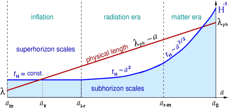
Figure 3: Evolution of a quantum particle’s physical wave length $\lambda_{\rm ph}=a(t)\lambda$ as the universe expands. Wave lengths which are now of cosmological size were originally minuscule. First horizon crossing occurs (at $a_{x}$) when $\lambda_{\rm ph}$ becomes comparable to the inflationary Hubble radius $\sim c/H_{I}$. At first crossing massless, minimally coupled scalars and gravitons of that wave length are ripped out of the vacuum by the expansion of spacetime. These particles ride the subsequent evolution of the universe relatively undisturbed until the second horizon crossing at $\lambda_{\rm ph}\sim c/H(t)$. Then the particles manifest themselves as cosmological-scale correlations which could not have formed causally after inflation.

As indiated in Fig. 3, after the first horizon crossing particles evolve on superhorizon scales during inflation and subsequent eras, to cross an horizon again in the radiation or matter era. For later use we shall now show how to relate the scale factor at the second horizon crossing to the coordinate wave vector $\|\vec{k}\|$. To this end, it is convenient to use the redshift, $z\equiv a_{0}/a(t)-1$, rather than time to label events. This choice implies $a=a_{0}/(1+z)$. For simplicity, we assume perfect matter domination from matter-radiation equality ($z_{\rm eq}\simeq 3200$) to the present ($z_{0}=0$). From Eq. (LABEL:matdom) of Sec. I, we can solve for the time in terms of the redshift and express the instantaneous Hubble parameter $H(t)=2/3t$ in terms of $z$. If we multiply by the scale factor, we find

$$aH=a_{0}H_{0}\sqrt{1+z}.\qquad\mbox{(matter domination)}$$ (64)

For $z>z_{\rm eq}$ we assume perfect radiation domination. By following the same procedure with Eq. (LABEL:raddom), we find,

$$aH=a_{0}H_{0}\frac{1+z}{\sqrt{1+z_{\rm eq}}}.\qquad\mbox{(radiation domination)}$$ (65)

Suppose galaxies form at $z=10$. A physical wave length of 10 kpc would have experienced second horizon crossing during the radiation epoch at about $z_{2x}\simeq 1.5\times 10^{7}$. Therefore the scales relevant to galaxy formation crossed during the radiation era, and we conclude that

$$\frac{a_{0}H_{0}z_{2x}}{\sqrt{z_{\rm eq}}}\simeq c\|\vec{k}\|\Longrightarrow a_{2x}\simeq\frac{a_{0}}{z_{2x}}=\frac{a_{0}^{2}H_{0}}{\sqrt{z_{\rm eq}}c\|\vec{k}\|}\,.$$ (66)

We have so far discussed only the fate of virtual particles that happen to emerge from the vacuum. The amount of particle production also depends upon the rate at which they emerge. Most types of massless particles possess a symmetry that makes this rate decrease as the universe expands. So any of these particles which emerge with $c\|\vec{k}_{\rm ph}\|\mathrel{\raise 1.29167pt\hbox{$<$\kern-7.5pt\lower 4.30554pt\hbox{$\sim$}}}H_{I}$ can persist forever without violating the uncertainty principle, but not many emerge.

This symmetry is called conformal invariance. Particle physicists find it convenient to describe symmetries, and all the other properties of a dynamical system, in terms of the system’s Lagrangian. In the classical mechanics of point particles the Lagrangian is the difference between the kinetic and potential energies, but the concept can be generalized to describe any sort of system, including the quantum field theories responsible for the vacuum polarization effect described in Sec. II. A field theory is said to be conformally invariant if its Lagrangian density (the Lagrangian is the spatial integral of the Lagrangian density) is unchanged when we multiply each field by a certain power of an arbitrary function of space and time $\Omega(x)$. Some interesting fields are the metric $g_{\mu\nu}$, the vector potential $A_{\mu}$, the Dirac field $\psi_{b}$ (with $b=1,2,3,4$) of spin $\frac{1}{2}$ particles, and the scalar field $\phi$. Their conformal transformations are,

$$g_{\mu\nu}\rightarrow\Omega^{2}g_{\mu\nu},\quad A_{\mu}\rightarrow A_{\mu},\quad\psi_{b}\rightarrow\Omega^{-\frac{3}{2}}\psi_{b},\quad\phi\rightarrow\Omega^{-1}\phi\,.$$ (67)

A typical conformally invariant Lagrangian density is that of electromagnetism,

$${\cal L}_{EM}=-\frac{1}{4}F_{\alpha\beta}F_{\rho\sigma}g^{\alpha\rho}g^{\beta\sigma}\sqrt{-g},$$ (68)

where $g={\rm det}(g_{\mu\nu})$ denotes the determinant of the metric and $g^{\mu\nu}$ is its matrix inverse.

Conformal invariance is so important because there is a coordinate system in which a general homogeneous and isotropic metric, Eq. (5), is just a conformal factor times the metric of flat space. The change of variables is defined by the differential relation, $d\eta=dt/a(t)$,

$$ds^{2}=-dt^{2}+a^{2}(t)d\vec{x}\cdot d\vec{x}=a^{2}[-d\eta^{2}+d\vec{x}\cdot d\vec{x}]\,.$$ (69)

In the $(\eta,\vec{x})$ coordinate system — which we shall henceforth employ, except as noted — the metric and its inverse are,

$$g_{\mu\nu}=a^{2}\eta_{\mu\nu},\qquad g^{\mu\nu}=a^{-2}\eta^{\mu\nu}\,,$$ (70)

where $\eta_{\mu\nu}=\eta^{\mu\nu}={\rm diag}(-1,1,1,1)$. In this coordinate system, a conformally invariant Lagrangian density is the same as in flat space when expressed in terms of the conformally rescaled fields Eq. (67) with $\Omega=a^{-1}$. For example, the Lagrangian densities of electromagnetism, massless Dirac fermions, and a massless, conformally coupled, complex scalar are,

$${\cal L}_{EM} = -\frac{1}{4}F_{\alpha\beta}F_{\rho\sigma}\eta^{\alpha\rho}\eta^{\beta\sigma}\,,$$ (71)

$${\cal L}_{D} = i(a^{\frac{3}{2}}{\overline{\psi}}_{b})\gamma_{bc}^{\mu}\partial_{\mu}(a^{\frac{3}{2}}\psi_{c})\,,$$ (72)

$${\cal L}_{CS} = -\partial_{\mu}(a\phi^{*})\partial_{\nu}(a\phi)\eta^{\mu\nu}\,.$$ (73)

where $\gamma^{\mu}_{bc}$ (with $b,c=1,2,3,4$) are the gamma matrices of Dirac theory PeskinSchroeder:1995 .

Although the formalism of Lagrangian quantum field theory is a straightforward generalization of quantum mechanics, the reader who is unfamiliar with it need not fret over how Lagrangians and Lagrangian densities encapsulate the dynamics of any particular system; it is sufficient for our discussion to note that they do. Therefore, any two systems whose Lagrangians agree have the same dynamics. We shall exploit this fact at several points in the subsequent discussion, starting now. Because the massless particle Lagrangian densities in Eqs. (71)–(73) agree for the conformally rescaled fields with those of flat space, it follows that the rate at which virtual particles emerge from the vacuum is the same in conformal coordinates as it is in flat space. Let us call this constant rate $\Gamma$. It gives the number of virtual particles emerging per unit conformal time $\eta$. This means that the number per unit physical time $t$ is,

$$\frac{dn}{dt}=\frac{d\eta}{dt}\frac{dn}{d\eta}=\frac{\Gamma}{a}\,.$$ (74)

Hence the emergence rate falls like $1/a(t)$ in physical time, and we see that the production of massless, conformally invariant particles is highly suppressed.

Readers who have studied undergraduate quantum mechanics are familiar with the minimal coupling prescription by which one generalizes the Schrödinger equation to account for the interaction of a point particle with an electromagnetic field. What one does is to replace the derivative operator $\partial_{\mu}$ everywhere with the covariant derivative $\partial_{\mu}+i(e/\hbar c)A_{\mu}(x)$, where $e$ is the particle’s charge and $A_{\mu}(x)$ is the 4-vector potential evaluated at the particle’s position in spacetime. A very similar procedure exists for generalizing the dynamics of any system from flat space to curved space. This prescription is also called minimal coupling. For electromagnetism and massless Dirac fermions it happens to produce the conformally invariant Lagrangian densities Eqs. (71) and (72). However, when a massless scalar is minimally coupled, the Lagrangian density which results is not Eq. (73), but rather,

$${\cal L}_{MS}=-\partial_{\mu}\phi^{*}\partial_{\nu}\phi g^{\mu\nu}\sqrt{-g}=-a^{2}\partial_{\mu}\phi^{*}\partial_{\nu}\phi\eta^{\mu\nu}.$$ (75)

This Lagrangian density is not conformally invariant, which means that the rate at which massless, minimally coupled scalars emerge from the vacuum per unit physical time need not fall off like the rates (74) of other massless particles. We shall now show, by direct calculation, that it does not.

Recall that the Lagrangian of any field theory is obtained by integrating the Lagrangian density over space. Doing this in the original $(t,\vec{x})$ coordinate system for Eq. (75) and applying Parseval’s theorem gives

$$L_{MS} = \int d^{3}x{\cal L}_{MS}$$

$$= \frac{a^{3}(t)}{c^{2}}\int\!\!\frac{d^{3}k}{(2\pi)^{3}}\Bigl{\{}|\widetilde{\dot{\phi}}(t,\vec{k})|^{2}-\frac{\|c\vec{k}\|^{2}}{a^{2}(t)}|\widetilde{\phi}(t,\vec{k})|^{2}\Bigr{\}}.\quad$$

Now note that integration is a form of summation. The correspondence can be made explicit by changing to dimensionless variables $\vec{k}=2\pi\vec{n}H_{I}/c$, and then exploiting the Maclaurin relation between sums and integrals (familiar from undergraduate statistical mechanics),

$$\int\!\!\frac{d^{3}k}{(2\pi)^{3}}=\Bigl{(}\frac{H_{I}}{c}\Bigr{)}^{3}\!\int d^{3}n\longrightarrow\Bigl{(}\frac{H_{I}}{c}\Bigr{)}^{3}\sum_{\vec{n}}\,.$$ (77)

We can define point particle positions using the real and imaginary parts of $\widetilde{\phi}(t,\vec{k})$,

$$\widetilde{\phi}(t,\vec{k})\equiv\sqrt{\frac{\hbar c^{3}}{2H_{I}^{2}}}\Bigl{(}x(t,\vec{n})+iy(t,\vec{n})\Bigr{)}\,.$$ (78)

Hence the scalar Lagrangian,

$$L_{MS}\longrightarrow\frac{\hbar H_{I}a^{3}}{2c^{2}}\sum_{\vec{n}}\Bigl{\{}\dot{x}^{2}+\dot{y}^{2}-\Bigl{(}\frac{c\|\vec{k}\|}{a}\Bigr{)}^{2}(x^{2}+y^{2})\Bigr{\}},$$ (79)

reveals that each wave vector of the scalar corresponds to two independent harmonic oscillators with the following time dependent mass and frequency,

$$m(t)=c^{-2}\hbar H_{I}a^{3}(t)\quad{\rm and}\quad\omega(t)=c\|\vec{k}\|/a(t)\,.$$ (80)

Harmonic oscillators with a time dependent mass and frequency have been much studied in quantum mechanics Gasiorowicz:1974 . The minimum energy at time $t$ is well known to be $\frac{1}{2}\hbar\omega(t)$, however, the state with this energy does not generally evolve onto itself. For the inflationary case of $a(t)\propto e^{H_{I}t}$, the system’s time dependence can be solved exactly. The state whose energy is minimum in the distant past has instantaneous average (zero-point) energy,

$$E_{0\!-\!point}(t,\vec{k})=\frac{\hbar c\|\vec{k}\|}{a(t)}+\frac{\hbar H_{I}^{2}a(t)}{2c\|\vec{k}\|}\,.$$ (81)

The second term in Eq. (81) is attributable to particle production. The energy of a single particle with this wave vector is $\hbar c\|\vec{k}\|/a(t)$, so the average number of particles with wave vector $\vec{k}$ is,

$$N(t,\vec{k})=\frac{1}{2}\Bigl{(}\frac{H_{I}a(t)}{c\|\vec{k}\|}\Bigr{)}^{2}\,.$$ (82)

As we expect, $N(t,\vec{k})$ is small for very early times and becomes comparable to one at horizon crossing. If we sum the contributions from all wave vectors that have experienced horizon crossing and divide by the spatial volume, we find the number density,

$$\frac{N}{V}=\frac{H_{I}^{3}}{4\pi^{2}c^{3}}\,.$$ (83)

This corresponds to $1/8\pi^{2}$ particles per Hubble volume for each degree of freedom.

We close by commenting that there can be no question about the reality of inflationary particle production because its impact has been detected. There is strong evidence that it is what caused the anisotropies imaged by WMAP Bennett:wmap2003 . Indeed, all the cosmological structures of the current universe are the result of gravitational collapse into these (originally) quantum fluctuations over the course of 13.7 billion years!

IV Vacuum polarization in inflation

The inflationary Hubble parameter Eq. (22) corresponds to an enormous energy,

$$\hbar H_{I}\simeq 10^{3}~{}{\rm J}\simeq 10^{13}\,{\rm GeV}\,.$$ (84)

On this scale all the charged particles in the Standard Model of particle physics are effectively massless. Even a particle we normally consider very massive, such as the $t$ quark, has less than $10^{-10}$ times as much rest mass energy. However, all but one of the Standard Model charged particles are described by the Dirac field $\psi_{a}$, whose Lagrangian density, Eq. (72), becomes conformally invariant when we ignore masses. As explained in Sec. III, conformally invariant particles are not produced much during inflation. This means that they do not contribute much more to the polarization of the vacuum during inflation than they do in flat space.

The lone exception within the Standard Model of elementary particle theory is the charged sector of the Higgs scalar. At low energy it manifests as the longitudinal component of the $W^{\pm}$. Its mass of about 80 GeV is also insignificant on the scale of inflation. No one really knows how it couples to the metric, but the usual assumption, based on how the field renormalizes, is minimal coupling. We can therefore model it with the Lagrangian density of a massless, charged and minimally coupled scalar,

$${\cal L}_{SQED}\! = \!-(\partial_{\mu}-ie^{\prime}A_{\mu})\phi^{*}(\partial_{\nu}+ie^{\prime}A_{\nu})\phi g^{\mu\nu}\sqrt{-g}\quad$$ (85)

$$= \!-a^{2}(\partial_{\mu}-ie^{\prime}A_{\mu})\phi^{*}(\partial_{\nu}+ie^{\prime}A_{\nu})\phi\eta^{\mu\nu}.$$

(Here $e^{\prime}\equiv e/\hbar c$, and $e\simeq-0.30\sqrt{\hbar c}$ is the charge of the electron. The subscript SQED stands for scalar quantum electrodynamics.) There may be more so-far undiscovered charged scalars of this type lurking between the $\sim 10^{2}$ GeV energies which can be explored at accelerators and the enormous energy in Eq. (84) of the inflationary Hubble parameter.

With Ola Törnkvist we have computed the vacuum polarization from ${\cal L}_{SQED}$ ProkopecTornkvistWoodard:2002 ; ProkopecTornkvistWoodard:2002b . In the $x^{\mu}=(\eta,\vec{x})$ coordinates Eq. (69) our result for the polarization bi-tensor takes the same form Eq. (42) as it does for the linear, isotropic medium discussed in Sec. II. With the scale factor normalized to unity at the start of inflation the two scalar functions are,

$$\chi_{e}(x,x^{\prime}) = \chi_{e}^{\rm flat}\!(x,x^{\prime})-\frac{\alpha}{6\pi}\ln(a)\delta^{4}(x-x^{\prime})$$

$$\;+\,\frac{\alpha aa^{\prime}H_{I}^{2}}{8\pi^{2}c^{2}}\!\!\!\!\! \!\!\!\!\!\!\partial^{2}\Bigl{\{}\theta(\Delta\eta)\theta(\Delta\tau^{2})[1+\ln(H_{I}^{2}{\Delta\tau}^{2})]\Bigr{\}}\quad$$ (86)

$$\delta n^{2}(x,x^{\prime}) = \frac{\alpha a^{2}a^{\prime 2}H_{I}^{4}}{4\pi^{2}c^{4}}\theta(\Delta\eta)\theta({\Delta\tau}^{2})[2+\ln(H_{I}^{2}{\Delta\tau}^{2})]$$

Here ${\Delta\eta}\equiv\eta-\eta^{\prime}$ and $\Delta\tau^{2}\equiv(\eta-\eta^{\prime})^{2}-c^{-2}\|\vec{x}-\vec{x}^{\prime}\|^{2}$. $\chi_{e}^{\rm flat}\!(x,x^{\prime})$ is the flat space result (59), with $t$ and $t^{\prime}$ replaced by $\eta$ and $\eta^{\prime}$. This term is renormalized precisely as in flat space, and contains no scale factors. The inflationary corrections are completely finite and depend on the scale factors $a\equiv a(\eta)$ and $a^{\prime}\equiv a(\eta^{\prime})$. These inflationary corrections come from the long wave length virtual particles that are ripped out of the vacuum by the inflationary Hubble flow. This should obviously increase polarization because it fills spacetime with a plasma of charged particles.

A significant feature of our result is nonzero $\delta n^{2}(x,x^{\prime})$. Recall that it must always vanish in flat space quantum field theory by virtue of the Lorentz symmetry between space and time. The time-dependent metric of inflation, Eq. (70), does not possess this symmetry, so $\delta n^{2}(x,x^{\prime})\neq 0$. In terms of electrodynamics, this means that ${\cal L}_{SQED}$ induces a relative permittivity which is not the inverse of the permeability, so the index of refraction is not unity even in “empty” space.

Because the inflationary metric is time dependent, we cannot calculate the mass of the photon by checking for a pole in the Fourier transform of the susceptibility as we did in flat space, Eq. (48). A better way to proceed is by comparison with the Proca Lagrangian density which governs the dynamics of a fundamental massive photon,

$${\cal L}_{\rm P}\! \equiv \!-\frac{1}{4}F_{\alpha\beta}F_{\rho\sigma}g^{\alpha\rho}g^{\beta\sigma}\!\sqrt{-g}-\frac{m_{\gamma}^{2}c^{2}}{2\hbar^{2}}A_{\mu}A_{\nu}g^{\mu\nu}\!\sqrt{-g}$$ (88)

$$= \!-\frac{1}{4}F_{\alpha\beta}F_{\rho\sigma}\eta^{\alpha\rho}\eta^{\beta\sigma}-\frac{m_{\gamma}^{2}c^{2}}{2\hbar^{2}}A_{\mu}A_{\nu}\eta^{\mu\nu}a^{2}.$$

The field equations associated with this Lagrangian density are,

$$\eta^{\mu\nu}\eta^{\rho\sigma}\partial_{\rho}F_{\sigma\nu}-c^{2}\hbar^{\!-2}m_{\gamma}^{2}\eta^{\mu\nu}A_{\nu}a^{2}=0\,.$$ (89)

The mass term is distinguished by its factor of $a^{2}$.

Now recall Maxwell’s equations with vacuum polarization, Eq. (41), which we rewrite without the current,

$$\eta^{\mu\nu}\eta^{\rho\sigma}\partial_{\rho}F_{\sigma\nu}(x)+\!\int\!d^{4}x^{\prime}[\mbox{}^{\mu}\Pi^{\nu}]\!(x,x^{\prime})A_{\nu}(x^{\prime})=0.$$ (90)

We also recall the polarization bi-tensor Eq. (42),

$$[^{\mu}\Pi^{\nu}]\!(x,x^{\prime}) \equiv -[\eta^{\mu\nu}\eta^{\rho\sigma}-\eta^{\mu\rho}\eta^{\sigma\nu}]\partial^{\prime}_{\rho}\partial_{\sigma}\chi_{e}(x,x^{\prime})$$ (91)

$$+ \eta^{\mu i}\eta^{\nu j}[\delta_{ij}\partial^{\prime}_{k}\partial_{k}-\partial^{\prime}_{i}\partial_{j}]\delta n^{2}(x,x^{\prime})\,.\quad$$

We see from Eq. (LABEL:SQED2) that $\delta n^{2}(x,x^{\prime})$ contributes a factor of $a^{2}$. The $\chi_{e}(x,x^{\prime})$ term, Eq. (86), has at most a single factor of $a$, but note from $\partial_{\sigma}a=\delta^{0}_{\sigma}H_{I}a^{2}$ that this term can also give an $a^{2}$ in Eq. (90). A comparison with the Proca equations (89) suggests $m_{\gamma}\sim\sqrt{\alpha}H_{I}\hbar/c^{2}$.

We can obtain a quantitative result by solving Eq. (90) perturbatively in $\alpha$. First expand the vector potential in a series of terms $A_{\mu}^{(n)}\!(x)$ which go like $\alpha^{n}$,

$$A_{\mu}(x)=A_{\mu}^{(0)}\!(x)+A_{\mu}^{(1)}\!(x)+\dots$$ (92)

Now recall that the polarization bi-tensor is first order in $\alpha$, and it groups the terms in Eq. (90) in powers of $\alpha$. We see that $A_{\mu}^{(0)}\!(x)$ obeys the classical equation,

$$\eta^{\rho\sigma}\partial_{\rho}F^{(0)}_{\sigma\nu}\!(x)=0,$$ (93)

the general solution of which consists, in the Coulomb gauge, of a superposition of transverse plane waves,

$$A_{\mu}^{(0)}\!(x)=\epsilon_{\mu}(\vec{k})e^{-ic\|\vec{k}\|\eta+i\vec{k}\cdot\vec{x}}\,,\quad{\rm where}\ \epsilon_{0}=0=k_{i}\epsilon_{i}.\quad$$ (94)

The order $\alpha$ correction obeys,

$$\eta^{\mu\nu}\eta^{\rho\sigma}\partial_{\rho}F^{(1)}_{\sigma\nu}\!(x)\!+\!\int\!d^{4}x^{\prime}[\mbox{}^{\mu}\Pi^{\nu}](x,x^{\prime})A^{(0)}_{\nu}\!(x^{\prime})=0.$$ (95)

Now substitute Eq. (94) and evaluate the integral assuming the photon experienced first horizon crossing (see Fig. 3) long before, and after a long period of inflation,

$$a\gg\frac{c\|\vec{k}\|}{H_{I}}\gg 1\,.$$ (96)

After some tedious expansions, the result is,

$$\int\!d^{4}x^{\prime}[^{\mu}\Pi^{\nu}](x,x^{\prime})A^{(0)}_{\nu}(x^{\prime})$$

$$= \!\!-\alpha c^{-2}H_{I}^{2}\eta^{\mu\nu}A_{\nu}^{(0)}(x)\Bigl{[}\frac{2}{\pi}\ln\Bigl{(}\frac{c\|\vec{k}\|}{H_{I}}\!\Bigr{)}+O(1)\Bigr{]}a^{2}+O(a).$$

The analogous first order Proca equation,

$$\eta^{\mu\nu}\eta^{\rho\sigma}\partial_{\rho}F^{(1)}_{\sigma\nu}-c^{2}\hbar^{\!-\!2}m_{\gamma}^{2}\eta^{\mu\nu}A^{(0)}_{\nu}a^{2}=0\,,$$ (98)

implies that the photon mass must be,

$$m_{\gamma}=\sqrt{\alpha}c^{-\!2}\hbar H_{I}\Bigl{[}\frac{2}{\pi}\ln\Bigl{(}\frac{c\|\vec{k}\|}{H_{I}}\!\Bigr{)}+O(1)\Bigr{]}^{\frac{1}{2}}.$$ (99)

We have thus discovered that the photon of scalar electrodynamics acquires mass during inflation.

V Hartree approximation

A simple way of obtaining almost the same result was previously suggested by one of us (Prokopec) in collaboration with Anne-Christine Davis, Konstantinos Dimopoulos, and Ola Törnkvist DavisDimopoulosProkopecTornkvist:2000 ; TornkvistDavisDimopoulosProkopec:2000 ; DimopoulosProkopecTornkvistDavis:2001 . The technique is to pretend that photons move in the quantum mechanical average of the scalar field. This is known as the Hartree or mean field approximation. First year graduate students should be familiar with its use in quantum mechanics to treat interacting, multi-electron atoms, and in statistical mechanics to treat interacting, multi-particle systems such as gases subject to the van der Waals force.

To implement the Hartree approximation we first take the average of ${\cal L}_{SQED}$ in Eq. (85) over quantum mechanical fluctuations of the scalar field. Of course this average eliminates the scalar fields, but it leaves behind some function of the vector potential,

$$\Bigl{\langle}{\cal L}_{SQED}\Bigr{\rangle} = -\Bigl{\langle}\partial_{\mu}\phi^{*}\partial_{\nu}\phi\Bigr{\rangle}\eta^{\mu\nu}a^{2}$$ (100)

$$+ \frac{ie}{\hbar c}\Bigl{\langle}\phi^{*}\partial_{\mu}\phi-\partial_{\mu}\phi^{*}\phi\Bigr{\rangle}A_{\nu}\eta^{\mu\nu}a^{2}$$

$$- \frac{e^{2}}{\hbar^{2}c^{2}}\Bigl{\langle}\phi^{*}\phi^{*}\Bigr{\rangle}A_{\mu}A_{\nu}\eta^{\mu\nu}a^{2}.$$

Now add this function to the Maxwell Lagrangian density Eq. (68).

By using the sophisticated techniques of quantum field theory, we can show that the quantum average of the scalar’s norm-squared consists of a divergent constant plus a finite term that grows like the logarithm of the scale factor scalarvev :

$$\Bigl{\langle}\phi^{*}(x)\phi(x)\Bigr{\rangle}={\rm U.V.}+\frac{H_{I}^{2}\hbar}{4\pi^{2}c}\ln(a)\,.$$ (101)

The other averages in Eq. (100) are either zero or else they do not multiply functions of the vector potential. The Hartree approximation Lagrangian density is therefore,

$${\cal L}_{\rm Hartree} = -\frac{1}{4}F_{\alpha\beta}F_{\rho\sigma}\eta^{\alpha\rho}\eta^{\beta\sigma}+{\rm U.V.}$$ (102)

$$- \frac{e^{2}}{\hbar^{2}c^{2}}\Bigl{[}{\rm U.V.}+\frac{H_{I}^{2}\hbar}{4\pi^{2}c}\ln(a)\Bigr{]}A_{\mu}A_{\nu}\eta^{\mu\nu}a^{2}.\qquad$$

Expression (102) contains ultraviolet divergences because virtual particles of arbitrarily large wave vector contribute to the average. This is the same origin as the divergences we found in Sec. II, and it is the ultimate origin of all ultraviolet divergences in quantum field theory. The only thing that need concern us here is the dependence of the divergent terms on the electromagnetic vector potential $A_{\mu}(x)$. The divergence without any vector potentials is harmless, but the other one could only be renormalized using a fundamental photon mass, which we do not have. This is one reason why the vacuum polarization — which can be consistently renormalized — is the correct way to study the kinematical properties of photons. But let us simply ignore the divergences in Eq. (102). A comparison of the finite parts with the Proca Lagrangian density Eq. (88) suggests the correspondence,

$$m_{\gamma}\Longleftrightarrow\sqrt{\alpha}c^{\!-\!2}\hbar H_{I}\Bigl{[}\frac{2}{\pi}\ln(a)\Bigr{]}^{\frac{1}{2}}\,.$$ (103)

Complete agreement with Eq. (99) requires only the additional assumption that the growth of Eq. (103) ceases for the mode of wave vector $\vec{k}$ (which we assume obeys $\|\vec{k}\|\gg H_{I}/c$) when it experiences horizon crossing, $a=c\|\vec{k}\|/H_{I}$ (see Fig. 3). This point of view is consistent with the causal picture according to which a photon’s mass only receives contributions from virtual scalars whose wave lengths are greater than the photon’s wave length.

We conclude this section by commenting on the size of the photon mass induced by our mechanism. During inflation we have $m_{\gamma}\sim 10^{13}\,{\rm GeV}/c^{2}$, which is enormous compared to the center-of-mass energies of $\sim 100\,{\rm GeV}$ attainable in the largest accelerators. A photon mass is not detected today because our result derives from the huge density of free charged particles ripped out of the vacuum by inflation. This plasma has been thoroughly dissipated at any wave length we can access in today’s laboratories.

According to the supernovae results Perlmutter-etal:1998 ; Riess-etal:1998 , the current universe may be entering another phase of inflation. This late inflationary phase also leads to a nonzero photon mass, but with the replacement of $H_{I}$ by the vastly smaller Hubble parameter of today, $H_{0}$. This substitution in Eq. (99) gives a minuscule photon mass, $m_{\gamma}\sim 10^{-42}\,{\rm GeV}/c^{2}$, which is far below the best current laboratory bounds of $m_{\gamma}\mbox{\raisebox{-2.58334pt}{~{}$\stackrel{{\scriptstyle<}}{{\sim}}$~{}}}10^{-49}\,{\rm kg}\approx 10^{-23}\,{\rm GeV/c^{2}}$ WilliamsFallerHill:1971 ; GoldhaberNieto:1971 .

VI Cosmological magnetic fields

The phenomenon of nonzero photon mass during inflation offers a fascinating 4-dimensional analogue to the Schwinger model in two dimensions Schwinger:1962 . However, it was proposed DavisDimopoulosProkopecTornkvist:2000 ; TornkvistDavisDimopoulosProkopec:2000 ; DimopoulosProkopecTornkvistDavis:2001 not for aesthetic appeal, but rather to explain the curious fact that galaxies seem to possess magnetic fields, which are correlated on scales of a few kilo-parsecs, and whose strength is typically a few micro-Gauss Kronberg:1994 . (The conversion factors to MKSA units are $1\,{\rm J/m}^{3}=10\,{\rm Gauss}^{2}$ and $10\,{\rm kpc}\simeq 3.1\times 10^{20}\,{\rm m}$.) There is also evidence that galactic clusters possess micro-Gauss magnetic fields correlated on scales of 10–100 kpc GrassoRubinstein:2001 . Although some of the material in this section is more technical than before, we present it to illustrate how the phenomenon of vacuum polarization during inflation may have left an observable consequence.

The difficulty with cosmic magnetic fields is not their field strengths but rather their enormous coherence lengths. A galaxy’s differential rotation can combine with the turbulent motion of ionized gas to power a phenomenon known as the $\alpha$-$\omega$ dynamo dynamo . In this mechanism the lines of a coherent seed field are stretched by rotation, twisted by turbulence, and then recombined to result in an exponential amplification, $B(t)\propto e^{t/\tau}$. Kinetic energy from the turbulent motion is converted into magnetic field energy in this way until equipartition is reached. Although many astrophysicists question the $\alpha$-$\omega$ dynamo, it is significant that the measured field strengths are at roughly the equipartition limit GrassoRubinstein:2001 .

There is no general agreement on a reasonable value for the dynamo time constant $\tau$; estimates vary from 0.2 to 0.8 billion years DavisLilleyTornkvist:1999 . By observing a surprisingly large polarization in the cosmic microwave background photons, the WMAP satellite has seen reionization from the first star formation at about 0.2 billion years into the 13.7 billion years of the universe’s existence Spergel:wmap2003 . One might expect large spiral galaxies to form at about 0.4 billion years DavisLilleyTornkvist:1999 , which implies dynamo operation for $13.7-0.4=13.3$ billion years, or between 17 to 66 time constants. Exponentiation results in amplification factors ranging from $e^{17}\simeq 2.4\times 10^{7}$ to as large as $e^{66}\simeq 4.6\times 10^{28}$. Therefore the cosmological magnetic fields of today might derive from correlated seeds as weak as $10^{-34}\,{\rm Gauss}$ at the time of galaxy formation. The real question is what produced the correlated seed fields in the hot, dense and very smooth early universe?

In the following, we argue that the nonzero photon mass of inflation might help to answer this question. As explained in Sec. III, a nonzero mass suppresses the creation of particles. On the other hand, it vastly enhances the zero-point energy that quantum mechanics predicts must reside in each photon wave vector $\vec{k}$, even if there are no particles with that wave vector anywhere in the universe. With no mass this zero-point energy falls as the universe expands,

$$E_{\gamma}(t,\vec{k})\Bigl{|}_{m_{\gamma}=0}=\frac{\hbar c\|\vec{k}\|}{2a(t)}\,.$$ (104)

A nonzero photon mass causes the zero-point energy of wave vectors that have experienced first horizon crossing to approach a constant instead,

$$E_{\gamma}(t,\vec{k})=\frac{1}{2}\sqrt{m_{\gamma}^{2}c^{4}+\hbar^{2}c^{2}\|\vec{k}\|^{2}/a^{2}}\longrightarrow\frac{1}{2}m_{\gamma}c^{2}\,.$$ (105)

After the end of inflation this wave vector eventually experiences second horizon crossing, $c\|\vec{k}\|\simeq a(t)H(t)$. If the mass goes to zero quickly thereafter, about half of the enormous zero-point energy must be shed in the form of long wave length photons at numbers vastly higher than thermal. The idea is that the mysterious seed fields derive from these long wave length photons becoming frozen in the plasma of the early universe.

Consider a wave vector $\vec{k}$ that is about to experience second horizon crossing. Each polarization of this system behaves as an independent harmonic oscillator whose frequency is suddenly changed from a large value $\Omega=m_{\gamma}c^{2}/\hbar$ to a much smaller one $\omega=c\|\vec{k}\|/a(t)$. Let $q$ and $p$ stand for the position and momentum operators of this oscillator. The Hamiltonians before and after are,

$$H_{B}=\frac{p^{2}}{2m}+\frac{1}{2}m\Omega^{2}q^{2},\qquad H_{A}=\frac{p^{2}}{2m}+\frac{1}{2}m\omega^{2}q^{2}\,.$$ (106)

Before transition the system is in its ground state,

$$H_{B}|0\rangle=\frac{1}{2}\hbar\Omega|0\rangle\,.$$ (107)

This result can be obtained from the standard relations,

$$q=\sqrt{\frac{\hbar}{2m\Omega}}\Bigl{(}\widehat{a}-\widehat{a}^{\dagger}\Bigr{)}\,,\quad p=\sqrt{\frac{\hbar m\Omega}{2}}\Bigl{(}-i\widehat{a}+i\widehat{a}^{\dagger}\Bigr{)},\quad$$ (108)

where $\widehat{a}=\widehat{a}_{0}\exp(-i\Omega t)$ and $\widehat{a}^{\dagger}=\widehat{a}_{0}^{\dagger}\exp(i\Omega t)$ are the lowering and raising operators, respectively, with $\widehat{a}_{0}|0\rangle=\widehat{a}|0\rangle=0$, not to be confused with the scale factor $a(t)$. The kinetic and potential terms each contribute half,

$$\frac{1}{2m}\langle 0|p^{2}|0\rangle=\frac{1}{4}\hbar\Omega=\frac{1}{2}m\Omega^{2}\langle 0|q^{2}|0\rangle\,.$$ (109)

After the transition the system is no longer an eigenstate, but we can find its average energy from the fact that the expectation values of $p^{2}$ and $q^{2}$ are continuous,

$$\langle 0|H_{A}|0\rangle=\frac{1}{4}\hbar\Omega\Bigl{[}1+\frac{\omega^{2}}{\Omega^{2}}\Bigr{]}\approx\frac{1}{4}\hbar\Omega\,.$$ (110)

If we compare this energy with the post-transition eigenstates $(N+\frac{1}{2})\hbar\omega$, we see that the average occupation number after transition is,

$$N\!(\vec{k})\simeq\frac{\Omega}{4\omega}=\frac{m_{\gamma}ca}{4\hbar\|\vec{k}\|}\,.$$ (111)

The substitution in Eq. (111) of the scale factor at the second horizon crossing, $a=a_{2x}$ as given in Eq. (66), results in the average occupation number for each polarization of wave vector $\vec{k}$,

$$N\!(\vec{k})=\frac{m_{\gamma}H_{0}a_{0}^{2}}{4\sqrt{z_{\rm eq}}\hbar\|\vec{k}\|^{2}}\,.$$ (112)

(Recall that $k_{\rm ph}=\|\vec{k}\|/a_{0}$ is the physical wave number measured today.) To within factors of order unity, the temperature at time $t$ is $T=T_{0}a_{0}/a(t)$, where $T_{0}\simeq 2.73\,{\rm K}$ is the current temperature of the cosmic microwave background. The number of thermal photons of wave number $\vec{k}$ and a fixed polarization obeys the Planck distribution,

$$N_{\rm th}\!(\vec{k})=\Bigl{[}\exp\ \Bigl{(}{\frac{\hbar c\|\vec{k}\|}{k_{B}T_{0}a_{0}}}\Bigr{)}-1\Bigr{]}^{-1}\,\stackrel{{\scriptstyle IR}}{{\longrightarrow}}\;\frac{k_{B}T_{0}a_{0}}{\hbar c\|\vec{k}\|}\,,$$ (113)

where $k_{B}\simeq 1.38\times 10^{-23}\,{\rm J/K}$ is the Boltzmann constant and the final relation on the right applies in the long wave length (IR) limit. The ratio of $m_{\gamma}$ photons to thermal ones can be expressed in terms of the present-day physical wave length $\lambda_{0}$,

$$\frac{N(\vec{k})}{N_{\rm th}(\vec{k})} \simeq \frac{m_{\gamma}cH_{0}\lambda_{0}}{8\pi\sqrt{z_{\rm eq}}k_{B}T_{0}}$$ (114)

$$= \frac{\hbar H_{I}H_{0}\lambda_{0}}{8\pi\sqrt{z_{\rm eq}}ck_{B}T_{0}}\Bigl{[}\frac{2\alpha}{\pi}\ln\Bigl{(}\frac{2\pi ca_{0}}{H_{I}\lambda_{0}}\Bigr{)}\Bigr{]}^{\frac{1}{2}}.$$

Recall that we normalize the scale factor to one at the start of inflation. For models with a long period of inflation the final factor in square brackets is dominated by $\ln(a_{0})$, which might be quite large. We parameterize our ignorance of the number of inflationary e-foldings by defining,

$$\varepsilon\equiv\Bigl{[}\frac{2\alpha}{\pi}\ln\Bigl{(}\frac{2\pi ca_{0}}{H_{I}(10~{}{\rm kpc})}\Bigr{)}\Bigr{]}^{\frac{1}{2}}.$$ (115)

If we work out the other numbers, we obtain,

$$\frac{N(\vec{k})}{N_{\rm th}(\vec{k})}\simeq\varepsilon\times 10^{\!-\!4}\Bigl{(}\frac{\lambda_{0}}{\rm m}\!\Bigr{)}\simeq\varepsilon\times 10^{17}\Bigl{(}\frac{\lambda_{0}}{10\,{\rm kpc}}\Bigr{)}.$$ (116)

We see that $m_{\gamma}$ photons are negligible compared to thermal ones on the $\lambda_{0}\sim 0.002$ m scale of the cosmic microwave background, but they are enormously dominant on the $\lambda_{0}\sim 10$ kpc scale relevant to galaxies.

At first the energy in these photons is almost completely electric, but Maxwell’s equations carry it to the magnetic sector. The physical magnetic field in a homogeneous and isotropic geometry is,

$$B^{i}(t,\vec{x})=-\frac{1}{2}\epsilon^{ijk}F_{jk}(t,\vec{x})/a^{2}(t)\,.$$ (117)

If we assume that half of the energy of the massive photons winds up in these magnetic fields, we conclude that their spatial Fourier transforms obey,

$$\Bigl{\langle}\widetilde{B}^{i}(t,\vec{k})\widetilde{B}^{i}(t,\vec{q})\Bigr{\rangle} \!=\! (2\pi)^{3}\delta^{3}(\vec{k}+\vec{q})N(\vec{k})\frac{\hbar c\|\vec{k}\|}{a^{4}(t)},$$ (118)

$$\!=\! (2\pi)^{3}\delta^{3}(\vec{k}+\vec{q})\frac{\varepsilon\hbar H_{I}H_{0}a_{0}^{2}}{4\sqrt{z_{\rm eq}}c\|\vec{k}\|a^{4}}.\qquad$$ (119)

The quantity of interest is the magnetic field averaged over a region of coordinate size $\ell=\ell_{0}/a(t)$,

$$B^{i}(t,\vec{x};\ell_{0}) \equiv (2\pi\ell^{2})^{-\frac{3}{2}}\!\int\!\!d^{3}ye^{-\frac{\|\vec{x}-\vec{y}\|^{2}}{2\ell^{2}}}B^{i}(t,\vec{y}),\qquad$$ (120)

$$= \!\int\!\frac{d^{3}k}{(2\pi)^{3}}e^{i\vec{k}\cdot\vec{x}}e^{-\frac{1}{2}\ell^{2}\|\vec{k}\|^{2}}\widetilde{B}^{i}(t,\vec{k})\,.$$ (121)

$B^{i}(t,\vec{x};\ell_{0})$ is an operator, but its average is a number,

$$B^{2}(t,\ell_{0}) \equiv \Bigl{\langle}B^{i}(t,\vec{x};\ell_{0})B^{i}(t,\vec{x};\ell_{0})\Bigr{\rangle}$$ (122)

$$= \frac{\varepsilon\hbar H_{I}H_{0}(1+z)^{2}}{16\pi^{2}\sqrt{z_{\rm eq}}c\,\ell_{0}^{2}}.$$

If we plug in the known numbers, we find

$$B(t,\ell_{0})\simeq\sqrt{\varepsilon}\times 10^{-33}\,{\rm Gauss}\Bigl{(}\frac{1+z}{\ell_{0}/10\,{\rm kpc}}\Bigr{)}.$$ (123)

This value is already within the lower range of conceivable seed fields. Turbulent evolution might contribute a factor of ten by transferring power from small scales DavisDimopoulosProkopecTornkvist:2000 . An additional factor of $(\rho_{\rm gal}/\rho_{0})^{\frac{2}{3}}\simeq 3\times 10^{3}$ accrues from field compression when the proto-galaxy collapses. If we assume $\varepsilon\sim 1$ and galaxy formation at $z\sim 10$, we might expect field strengths of about $10^{-28}$ Gauss at $\ell_{0}\sim 10$ kpc.

It should be emphasized that this is just one of many potential explanations for cosmological magnetic fields GrassoRubinstein:2001 . This section’s analysis is also highly simplified. We need to better understand the process through which a given wave vector’s mass dissipates at second horizon crossing. A proper calculation would also require careful study of the dynamics of the electric and magnetic fields during the epochs of reheating, radiation domination, and matter domination.

- (1) E. Hubble, “A relation between distance and radial velocity among extra-galactic nebulae,” Proc. Nat. Acad. Sci. USA 15, 168–173 (1929).
- (2) C. W. Wirtz, “Notiz zur Radialbewegung der Spiralnebel,” Astronomische Nachrichten 216, 451 (1922); C. W. Wirtz, “De Sitters Kosmologie und die Radialbewegungen der Spiralnebel,” Astronomische Nachrichten 222, 21 (1924).
- (3) S. Perlmutter et al. [Supernova Cosmology Project Collaboration], “Measurements of Omega and Lambda from 42 high-redshift supernovae,” Astrophys. J. 517, 565–586 (1999) or arXiv:astro-ph/9812133.
- (4) A. G. Riess et al. [Supernova Search Team Collaboration], “Observational evidence from supernovae for an accelerating universe and a cosmological constant,” Astron. J. 116, 1009–1038 (1998) or arXiv:astro-ph/9805201.
- (5) C. L. Bennett et al., “First year Wilkinson microwave anisotropy probe (WMAP) observations: Preliminary maps and basic results,” arXiv:astro-ph/0302207.
- (6) D. N. Spergel et al., “First year Wilkinson microwave anisotropy probe (WMAP) observations: Determination of cosmological parameters,” arXiv:astro-ph/0302209.
- (7) B. Ratra and P. J. Peebles, “Cosmological consequences of a rolling homogeneous scalar field,” Phys. Rev. D 37, 3406–3427 (1988).
- (8) R. R. Caldwell, R. Dave and P. J. Steinhardt, “Cosmological imprint of an energy component with general equation-of-state,” Phys. Rev. Lett. 80, 1582–1585 (1998) or arXiv:astro-ph/9708069.
- (9) A. H. Guth, “The inflationary universe: A possible solution to the horizon and flatness problems,” Phys. Rev. D 23, 347–356 (1981).
- (10) A. A. Starobinsky, “A new type of isotropic cosmological models without singularity,” Phys. Lett. B 91, 99–102 (1980).
- (11) K. Sato, “Cosmological baryon number domain structure and the first order phase transition of a vacuum,” Phys. Lett. B 99, 66–70 (1981).
- (12) D. Kazanas, “Dynamics of the universe and spontaneous symmetry breaking,” Astrophys. J. 241, L59–L63 (1980).
- (13) J. D. Jackson, Classical Electrodynamics (John Wiley & Sons, New York, 1999), 3rd ed., Chap. 7.
- (14) M. E. Peskin and D. V. Schroeder, An Introduction to Quantum Field Theory (Addison-Wesley, Reading, MA, (1995), Chap. 7.
- (15) E. R. Williams, J. E. Faller, and H. A. Hill, “New experimental test of Coulomb’s law: A laboratory upper limit on the photon rest mass,” Phys. Rev. Lett. 26, 721–724 (1971).
- (16) A. S. Goldhaber and M. M. Nieto, “Terrestrial and extra-terrestrial limits on the photon mass,” Rev. Mod. Phys. 43, 277–296 (1971).
- (17) J. Schwinger, “Gauge Invariance and Mass II,” Phys. Rev. 128, 2425–2429 (1962).
- (18) L. Parker, Quantized fields and particle creation in expanding universes. I,” Phys. Rev. 183, 1057–1068 (1969).
- (19) S. Gasiorowicz, Quantum Physics (Wiley and Sons, Inc., New York, 1974), p. 361.
- (20) T. Prokopec, O. Törnkvist and R. Woodard, “Photon mass from inflation,” Phys. Rev. Lett. 89, 101301-1–101301-5 (2002) or arXiv:astro-ph/0205331.
- (21) T. Prokopec, O. Törnkvist, and R. P. Woodard, “One loop vacuum polarization in a locally de Sitter background,” Ann. Phys. 303, 251–274 (2003) or arXiv:gr-qc/0205130.
- (22) A.-C. Davis, K. Dimopoulos, T. Prokopec, and O. Törnkvist, “Primordial spectrum of gauge fields from inflation,” Phys. Lett. B 501, 165–172 (2001) or astro-ph/0007214.
- (23) O. Törnkvist, A.-C. Davis, K. Dimopoulos, and T. Prokopec, “Large scale primordial magnetic fields from inflation and preheating,” in Verbier 2000, Cosmology and particle physics (CAPP2000), 443–446, or astro-ph/0011278.
- (24) K. Dimopoulos, T. Prokopec, O. Törnkvist, and A.-C. Davis, “Natural magnetogenesis from inflation,” Phys. Rev. D 65, 063505-1–063505-26 (2002) or astro-ph/0108093.
- (25) A. Vilenkin and L. H. Ford, “Gravitational effects upon cosmological phase transitions,” Phys. Rev. D 26, 1231–1241 (1982) ; A. D. Linde, “Scalar field fluctuations in expanding universe and the new inflationary universe scenario,” Phys. Lett. B 116, 335-339 (1982); A. A. Starobinsky, “Dynamics of phase transitions in the new inflationary scenario and generation of perturbations,” Phys. Lett. B 117, 175–178 (1982).
- (26) P. P. Kronberg, “Extragalactic magnetic fields,” Rept. Prog. Phys. 57, 325–382 (1994).
- (27) D. Grasso and H. R. Rubinstein, “Magnetic fields in the early universe,” Phys. Rept. 348, 163–266 (2001) or astro-ph/0009061.
- (28) E. N. Parker, Cosmic Magnetic Fields (Clarendon, Oxford, 1979); Ya. B. Zeldovich, A. A. Ruzmaikin and D. D. Sokoloff, Magnetic Fields in Astrophysics (Gordon and Breach, New York, 1983).
- (29) A.-C. Davis, M. Lilley, and O. Törnkvist, “Relaxing the bounds on primordial magnetic seed fields,” Phys. Rev. D 60, 021301-1–021301-6 (1999) or astro-ph/9904022.