Determining Neutrino Mass from the CMB Alone

Abstract

Distortions of Cosmic Microwave Background (CMB) temperature and polarization maps caused by gravitational lensing, observable with high angular resolution and high sensitivity, can be used to measure the neutrino mass. Assuming two massless species and one with mass $m_{\nu}$ we forecast $\sigma(m_{\nu})=0.15$ eV from the Planck satellite and $\sigma(m_{\nu})=0.04$ eV from observations with twice the angular resolution and $\sim 20$ times the sensitivity. A detection is likely at this higher sensitivity since the observation of atmospheric neutrino oscillations require $\Delta m_{\nu}^{2}\mathrel{\mathchoice{\lower 3.6pt\vbox{\halign{$\mathsurround=0pt\displaystyle\hfil#\hfil$\cr>\crcr\sim\crcr}}}{\lower 3.6pt\vbox{\halign{$\mathsurround=0pt\textstyle\hfil#\hfil$\cr>\crcr\sim\crcr}}}{\lower 3.6pt\vbox{\halign{$\mathsurround=0pt\scriptstyle\hfil#\hfil$\cr>\crcr\sim\crcr}}}{\lower 3.6pt\vbox{\halign{$\mathsurround=0pt\scriptscriptstyle\hfil#\hfil$\cr>\crcr\sim\crcr}}}}(0.04{\rm eV})^{2}$.

Introduction. Results from the WMAP bennet03a show the standard cosmological model passing a highly stringent test. With this spectacular success of the CMB as a clean and powerful cosmological probe, and of the standard model as a phenomenological description of nature, it is timely to ask what can be done with yet higher resolution and higher sensitivity such as offered by the Planck instruments and beyond. In this Letter we mostly focus on neutrino mass determination, with brief discussion of other applications.

Eisenstein et al. eisenstein99 found that the Planck satellite can measure neutrino mass with an error of 0.26 eV. This sensitivity limit is related to the temperature at which the plasma recombines and the photons last scatter off of the free electrons, $T_{\rm dec}\simeq 0.3$ eV. Neutrinos with $m_{\nu}\mathrel{\mathchoice{\lower 3.6pt\vbox{\halign{$\mathsurround=0pt\displaystyle\hfil#\hfil$\cr<\crcr\sim\crcr}}}{\lower 3.6pt\vbox{\halign{$\mathsurround=0pt\textstyle\hfil#\hfil$\cr<\crcr\sim\crcr}}}{\lower 3.6pt\vbox{\halign{$\mathsurround=0pt\scriptstyle\hfil#\hfil$\cr<\crcr\sim\crcr}}}{\lower 3.6pt\vbox{\halign{$\mathsurround=0pt\scriptscriptstyle\hfil#\hfil$\cr<\crcr\sim\crcr}}}}T_{\rm dec}$ do not leave any imprint on the last-scattering surface that would distinguish them from $m_{\nu}=0$.

Neutrinos with mass $m_{\nu}\mathrel{\mathchoice{\lower 3.6pt\vbox{\halign{$\mathsurround=0pt\displaystyle\hfil#\hfil$\cr<\crcr\sim\crcr}}}{\lower 3.6pt\vbox{\halign{$\mathsurround=0pt\textstyle\hfil#\hfil$\cr<\crcr\sim\crcr}}}{\lower 3.6pt\vbox{\halign{$\mathsurround=0pt\scriptstyle\hfil#\hfil$\cr<\crcr\sim\crcr}}}{\lower 3.6pt\vbox{\halign{$\mathsurround=0pt\scriptscriptstyle\hfil#\hfil$\cr<\crcr\sim\crcr}}}}T_{\rm dec}$ would affect the amplitudes of gravitational potential peaks and valleys at intermediate redshifts. Massive neutrinos can collapse into potential wells when they become non-relativistic, while massless ones freely stream out. The observed galaxy power spectrum (which is proportional to the potential power spectrum at sufficiently large scales), combined with CMB observations can be used to put constraints on $m_{\nu}$ hu98a . At present such an analysis yields an upper bound on $m_{\nu}$ of $\sim 0.3$ eV spergel03 .

The alteration of the gravitational potentials at late times changes the gravitational lensing of CMB photons as they traverse these potentials seljak96 ; bernardeau97 . Including the gravitational lensing effect, we find that the Planck error forecast improves to 0.15 eV. We also show that more ambitious CMB experiments can reduce this error to $\sim 0.04$ eV. These mass ranges are interesting because the atmospheric neutrino oscillations require that at least one of the active neutrinos have $m_{\nu}>0.04$ to 0.1 eV. More detailed considerations beacom02 show that the sum of the active neutrino masses (which is what the CMB is most sensitive to) should be at least 0.06 eV.

Tomographic observations of the galaxy shear due to gravitational lensing can achieve sensitivities to $m_{\nu}$ similar to what we find here hu99 ; abazajian02b . Our work is distinguished by its sole reliance on CMB temperature and polarization maps which have different potential sources of systematic error. Complementary techniques are valuable since both of these will be very challenging measurements.

The most stringent laboratory upper bound on neutrino mass comes from tritium beta decay end-point experiments tritium which limit the electron neutrino mass to $\mathrel{\mathchoice{\lower 3.6pt\vbox{\halign{$\mathsurround=0pt\displaystyle\hfil#\hfil$\cr<\crcr\sim\crcr}}}{\lower 3.6pt\vbox{\halign{$\mathsurround=0pt\textstyle\hfil#\hfil$\cr<\crcr\sim\crcr}}}{\lower 3.6pt\vbox{\halign{$\mathsurround=0pt\scriptstyle\hfil#\hfil$\cr<\crcr\sim\crcr}}}{\lower 3.6pt\vbox{\halign{$\mathsurround=0pt\scriptscriptstyle\hfil#\hfil$\cr<\crcr\sim\crcr}}}}2$ eV. Proposed exeriments plan to reduce this limit by one to two orders of magnitude by searching for neutrinoless double beta decay ($\beta\beta 0\nu$) zdesenko03 . A Dirac mass would elude this search, but theoretical prejudice favors (and the see-saw mechanism requires) Majorana masses. Like the CMB and galaxy shear observations, these future $\beta\beta 0\nu$ experiments will be extremely challenging.

Lensing of the CMB. The intensity and linear polarization of the CMB are completely specified by the Stokes parameters, $I$, $Q$ and $U$ which are related to the unlensed Stokes parameters (denoted with a tilde) by $X({\bf n})=\tilde{X}({\bf n}+{\bf\delta n})$ where $X$ stands for $I$, $Q$ or $U$. The deflection angle, ${\bf\delta n}$, is the tangential gradient of the projected gravitational potential,

$$\phi({\bf n})=2\int dr\Psi(r{\bf\hat{n}},r)(r-r_{s})/(rr_{s})\,,$$ (1)

where $r$ is the coordinate distance along our past light cone, $s$ denotes the CMB last–scattering surface, ${\bf\hat{n}}$ is the unit vector in the ${\bf n}$ direction and $\Psi$ is the three-dimensional gravitational potential.

The statistical properties of the $I$, $Q$ and $U$ maps are most simply described in the transform space: $a_{T}({\bf l})$, $a_{E}({\bf l})$, and $a_{B}({\bf l})$ where $a_{T}$ is the spherical harmonic transform of $I$ and $a_{E}$ and $a_{B}$ are the curl–free and gradient–free decompositions, respectively, of $Q$ and $U$ kamionkowski97 ; seljak97 . In this transform space the effect of lensing by mode $\phi({\bf L})$ (harmonic transform of $\phi({\bf n})$) is to shift power from, e.g., $\tilde{a}_{T}({\bf L-l})$ to $a_{T}(\bf l)$. Lensing also mixes $\tilde{a}_{E}$ into $a_{B}$ and any $\tilde{a}_{B}$ into $a_{E}$ zaldarriaga98b , thus generating scalar B (curl) mode correlations.

Lensing smoothes out the features in the two-point functions, also called angular power spectra, ${\cal C}^{\alpha\alpha^{\prime}}_{l}$, where $\langle a_{\alpha}({\bf l})a^{*}_{\alpha^{\prime}}({\bf l^{\prime}})\rangle={\cal C}_{l}^{\alpha\alpha^{\prime}}\delta({\bf l}-{\bf l^{\prime}})/[2\pi l(l+1)]$ and $\alpha$ stands for $T$, $E$, or $B$ seljak96 . As explained later, in our analysis we use the unlensed power spectra, ${\tilde{\cal C}}^{\alpha\alpha^{\prime}}_{l}$. The information from lensing is added through the two-point function of the lensing potential, $\langle\phi({\bf L})\phi^{*}({\bf L^{\prime}})\rangle={\cal C}_{L}^{\phi\phi}\delta({\bf L}-{\bf L^{\prime}})/[2\pi L(L+1)]$, which can be inferred from the temperature and polarization map 4-point functions hu02b . In Figure 1 we plot the deflection angle power spectrum, ${\cal C}_{l}^{dd}\equiv l(l+1){\cal C}_{l}^{\phi\phi}$.

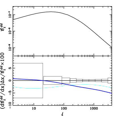
Figure 1: Top panel: Deflection angle power spectrum ${\cal C}_{l}^{dd}$ for the fiducial model ($m_{\nu}=0$). Bottom panel: $100\times d{\cal C}_{l}^{dd}/dm_{\nu}\times(\Delta m_{\nu}/{\cal C}_{l}^{dd})$ (dark) and $100\times d{\cal C}_{l}^{dd}/dw_{x}\times(\Delta w_{x}/{\cal C}_{l}^{dd})$ (light) for $\Delta m_{\nu}=0.1$ eV and $\Delta w_{x}=0.2$.

We calculate the 2-point functions using a publicly available code, CMBfast seljak96 , which was modified to include a scalar field dark energy component, to calculate ${\cal C}_{l}^{dd}$, and to include the effect of massive neutrinos on the recombination history (through the expansion rate). We use the Peacock and Dodds prescription to calculate the non-linear matter power spectrum peacock96 .

Effect of neutrinos. The lower panel in Figure 1 shows the differences in the power spectra between our fiducial model and the exact same model but with one of the three neutrino masses altered from zero to 0.1 eV. The error boxes are those for CMBpol (described below; see Table 1). The ${\cal C}_{l}^{dd}$ are noise-dominated at $l>600$ for CMBpol.

The signature of a 0.1 eV neutrino in the angular power spectra, in the absence of lensing, is at the 0.1% level. Such small masses are only detectable through their effect on lensing, which comes through their influence on the gravitational potential. Replacing a massless component with a massive one increases the energy density and therefore the expansion rate, suppressing growth. The net suppression of the power spectrum is scale dependent and the relevant length scale is the Jeans length for neutrinos bond83 ; ma96 ; hu98 which decreases with time as the neutrino thermal velocity decreases. This suppression of growth is ameliorated at scales larger than the Jeans length at matter–radiation equality, where the neutrinos can cluster. Neutrinos never cluster at scales smaller than the Jeans length today. The net result is no effect on large scales and a suppression of power on small scales, resulting in the shape of $\delta{\cal C}_{l}^{dd}/{\cal C}_{l}^{dd}$ in Figure 1.

Error forecasting method.

The power spectra we include in our analysis are ${\tilde{\cal C}}_{l}^{TT}$, ${\tilde{\cal C}}_{l}^{TE}$, ${\tilde{\cal C}}_{l}^{EE}$ (unlensed), and ${\cal C}_{l}^{dd}$. We do not use the lensed power spectra to avoid the complication of the correlation in their errors between different $\ell$ values and with the error in ${\cal C}_{l}^{dd}$. Using the lensed spectra and neglecting these correlations can lead to overly optimistic forecasts hu02a . If we include the lensed spectra instead of the unlensed ones, the expected errors on $w_{x}$ and $m_{\nu}$ for CMBpol (see Table 1) shrink by about 40% and 30% respectively.

The distortions to the angular power spectra due to a $0.1$ eV neutrino and changes of order 10% in $w_{x}$ are very small. We have taken care to accurately forecast the constraints possible in this mass range. First, we make a Taylor expansion of the power spectra to first order in all the cosmological parameters. Then, given the the expected experimental errors on the power spectra, the expected parameter error covariance matrix is easily calculated.

The Taylor expansion works better and susceptibility to numerical error is reduced with a careful choice of the parameters used to span a given model space eisenstein99 ; efstathiou99 ; hu01a ; kosowsky02 . We take our set to be ${\cal P}=\{\omega_{m},\omega_{b},\omega_{\nu},\theta_{s},w_{x},z_{\rm ri},k^{3}P_{\Phi}^{i}(k_{f}),n_{s},n_{s}^{\prime},y_{\rm He}\}$, with the assumption a flat universe. The first three of these are the densities today (in units of $1.88\times 10^{-29}{\rm g}/{\rm cm}^{3}$) of cold dark matter plus baryons, baryons and massive neutrinos. Next two are the angular size subtended by the sound horizon on the last–scattering surface and the ratio of dark energy pressure to density. The Thompson scattering optical depth for CMB photons, $\tau$, is parameterized by the redshift of reionzation $z_{\rm ri}$. The primordial potential power spectrum is assumed to be $k^{3}P_{\Phi}^{i}(k)=k_{f}^{3}P_{\Phi}^{i}(k_{f})(k/k_{f})^{n_{s}-1+n_{S}^{\prime}ln(k/k_{f})}$ with $k_{f}=0.05\,{\rm Mpc}^{-1}$. The fraction of baryonic mass in Helium is $y_{\rm He}$. We Taylor expand about ${\cal P}=\{0.146,0.021,0,0.6,-1,6.3,6.4\times 10^{-11},1,0,0.24\}$.

We follow zaldarriaga97 to calculate the errors expected in ${\tilde{\cal C}}_{l}^{TT}$, ${\tilde{\cal C}}_{l}^{TE}$ and ${\tilde{\cal C}}_{l}^{EE}$ given Table 1. For errors on ${\cal C}_{l}^{dd}$ we follow hu02b . The errors on the unlensed spectra in the regime where lensing is important (deep in the damping tail) are certainly underestimated because reconstruction of the unlensed map from the lensed map will add to the errors. However, this is not worrisome since we limit all the unlensed spectra to $l<2000$, and a further restriction to $l<1500$ (where lensing is least important) only increases the error on $m_{\nu}$ by about 10% for CMBpol.

Experiments. We consider Planck planck , a high-resolution version of CMBpol , and a polarized bolometer array on the South Pole Telescope we will call SPTpol. Their specifications are given in Table 1. We assume that other frequency channels of Planck and CMBpol (not shown in the table) will clean out non-CMB sources of radiation perfectly. Detailed studies have shown foreground degradation of the results expected from Planck to be mild knox99 ; tegmark00b ; bouchet99 . At $l>3000$ emission from dusty galaxies will be a significant source of contamination. The effect is expected to be more severe for temperature maps. Hence we restrict temperature data to $l<2000$ and polarization data to $l<2500$.

Experiment	$l_{\rm max}^{\rm T}$	$l_{\rm max}^{\rm E,B}$	$\nu$ (GHz)	$\theta_{b}$	$\Delta_{T}$	$\Delta_{P}$
Planck	2000	2500	100	9.2’	5.5	$\infty$
			143	7.1’	6	11
			217	5.0’	13	27
SPTpol ($f_{\rm sky}=0.1$)	2000	2500	217	0.9’	12	17
CMBpol	2000	2500	217	3.0’	1	1.4

Table 1: Experimental specifications. We use the unlensed spectra (${\tilde{\cal C}}_{l}^{TT}$, ${\tilde{\cal C}}_{l}^{TE}$, ${\tilde{\cal C}}_{l}^{EE}$) only at $l<2000$. For $\phi$ reconstruction we use only data with $l<l_{\rm max}^{T,E,B}$.

Table 2:

Error Forecasts
Experiment $m_{\nu}$ (eV) $w_{x}$ $\ln P_{\Phi}^{i}$ $n_{S}$ $n_{S}^{\prime}$ $\theta_{s}$ (deg) $\tau$ $\ln\omega_{m}$ $\ln\omega_{b}$ $y_{\rm He}$ Planck 0.15 0.31 0.017 0.0071 0.0032 0.002 0.0088 0.0066 0.0075 0.012 SPTpol 0.18 0.49 0.018 0.01 0.006 0.0026 0.0088 0.0087 0.01 0.017 CMBpol 0.044 0.18 0.017 0.0029 0.0017 0.00064 0.0085 0.0022 0.0028 0.0048
NOTES.—Standard deviations expected from Planck, SPTpol and CMBpol.

Results. We emphasize the ability of the experiments to simultaneously determine $P_{\Phi}^{i}$, $w_{x}$ and $m_{\nu}$ . These all affect the amplitude of $P_{\Phi}$ at late times, the latter two due to their effect on the rate of growth of density perturbations. If we were only sensitive to the amplitude of ${\cal C}_{l}^{dd}$ then there would be an exact degeneracy between these three parameters. However, the $l$-dependence of the response of ${\cal C}_{l}^{dd}$ to these parameter variations breaks this would-be degeneracy, allowing for their simultaneous determination.

The effect of $m_{\nu}$ can easily be disentangled from that of $w_{x}$. We have already discussed the $l$-dependence of $\partial\ln{\cal C}_{l}^{dd}/\partial m_{\nu}$ shown in Fig. 1 as resulting from the scale- and time-dependence of $\partial\ln P_{\Phi}/\partial m_{\nu}$. The $l$-dependence of $\partial\ln{\cal C}_{l}^{dd}/\partial w_{x}$ has the opposite sense. Although the suppression of $P_{\Phi}$ for increasing $w_{x}$ is nearly $k$–independent, the effect is larger at late times —hence the radial projection gives a larger effect at low $\ell$. The effects of $m_{\nu}$ and $w_{x}$ are sufficiently distinct to allow for their simultaneous determination. We point out that the effect of $w_{x}$ is more pronounced for larger values due to two reasons. One, dark energy starts to dominate earlier (which implies larger uniform suppression) and two, perturbations in dark energy on large scales are enhanced for large $w_{x}$.

The difference in the response of ${\cal C}_{l}^{dd}$ to $m_{\nu}$ and $w_{x}$ allows for, e.g., Planck to detect the acceleration of the Universe ($w_{x}<-1/(3\Omega_{x})$) at the 2$\sigma$ level. Such a confirmation would be valuable given the deep theoretical implications of acceleration kaloper02 . Hu hu02a has previously noted this result obtained with the assumption $m_{\nu}=0$.

As is well known, the $P_{\Phi}^{i}$ can be determined independently of the lensing signal, through use of a signal at large angular scales. One combines ${\cal C}_{l}^{EE}$ and ${\cal C}_{l}^{TE}$ at $l\mathrel{\mathchoice{\lower 3.6pt\vbox{\halign{$\mathsurround=0pt\displaystyle\hfil#\hfil$\cr<\crcr\sim\crcr}}}{\lower 3.6pt\vbox{\halign{$\mathsurround=0pt\textstyle\hfil#\hfil$\cr<\crcr\sim\crcr}}}{\lower 3.6pt\vbox{\halign{$\mathsurround=0pt\scriptstyle\hfil#\hfil$\cr<\crcr\sim\crcr}}}{\lower 3.6pt\vbox{\halign{$\mathsurround=0pt\scriptscriptstyle\hfil#\hfil$\cr<\crcr\sim\crcr}}}}20$ where they are proportional to $P_{\Phi}^{i}\tau^{2}$ and $P_{\Phi}^{i}\tau$ respectively zaldarriaga97 ; kaplinghat03a with the TT, EE and ET spectra at $20\mathrel{\mathchoice{\lower 3.6pt\vbox{\halign{$\mathsurround=0pt\displaystyle\hfil#\hfil$\cr<\crcr\sim\crcr}}}{\lower 3.6pt\vbox{\halign{$\mathsurround=0pt\textstyle\hfil#\hfil$\cr<\crcr\sim\crcr}}}{\lower 3.6pt\vbox{\halign{$\mathsurround=0pt\scriptstyle\hfil#\hfil$\cr<\crcr\sim\crcr}}}{\lower 3.6pt\vbox{\halign{$\mathsurround=0pt\scriptscriptstyle\hfil#\hfil$\cr<\crcr\sim\crcr}}}}l\mathrel{\mathchoice{\lower 3.6pt\vbox{\halign{$\mathsurround=0pt\displaystyle\hfil#\hfil$\cr<\crcr\sim\crcr}}}{\lower 3.6pt\vbox{\halign{$\mathsurround=0pt\textstyle\hfil#\hfil$\cr<\crcr\sim\crcr}}}{\lower 3.6pt\vbox{\halign{$\mathsurround=0pt\scriptstyle\hfil#\hfil$\cr<\crcr\sim\crcr}}}{\lower 3.6pt\vbox{\halign{$\mathsurround=0pt\scriptscriptstyle\hfil#\hfil$\cr<\crcr\sim\crcr}}}}2000$ where they are proportional to $P_{\Phi}^{i}e^{-2\tau}$.

If we assume a single-step transition for the ionization history Planck can achieve $\sigma(\tau)=0.005$ eisenstein99 . However, foreground contamination tegmark00b , and modeling uncertainty in the ionization history holder03 can increase this uncertainty. For these reasons we conservatively ignore polarization data at $l<30$ and instead set a prior, by hand, of $\sigma(\tau)=0.009$; including the $l<30$ polarization data would (perhaps artificially) achieve a smaller $\sigma(\tau)$. In the end, $\tau$ is determined (only slightly) better than this prior because there is some constraint on $P_{\Phi}^{i}$ from the lensing signal. Note that since $P_{\Phi}^{i}e^{-2\tau}$ is so well-determined, we always expect $\sigma(\ln P_{\Phi})=2\sigma(\tau)$, as we find..

An extended period of reionization, as suggested by the combination of WMAP and quasar observations kogut03 , may have large spatial fluctuations in the ionization fraction. Such “patchy” reionization would lead to a large diffuse kinetic SZ contribution to ${\cal C}_{l}^{TT}$ at high $l$ knox98 ; santos03 , possibly larger than the lensing contribution. Fortunately the analogous effect in the polarization is much smaller. For a conservative upper bound on how patchy reionization could degrade $\sigma(m_{\nu})$, we restrict the temperature data to $l<1000$ and find $\sigma(m_{\nu})=0.045$ eV for CMBpol and 0.34 eV for Planck.

The primary motivation for CMBpol is the detection of the B mode due to gravity waves produced in inflation. The amplitude of this signal would directly tell us the energy density during inflation. Following the calculation in knox02 ; kesden02 we find a $3\sigma$ detection is possible for CMBpol if the energy density during inflation is greater than $\rho_{\rm min}=(2\times 10^{15}{\rm GeV})^{4}$; $\rho_{\rm min}^{1/4}$ is an order of magnitude smaller than the GUT scale. We note that $\rho_{\rm min}\propto 1/\tau$, approximately, for $0.05<\tau<0.2$ and we have assumed $\tau=0.1$. This scaling with $\tau$ suggests that the reionization feature in the B mode at the largest angular scales is important and therefore a full-sky experiment is necessary to achieve this sensitivity level.

The scalar spectrum determined from high–resolution CMB observations (the constraining power comes from primary CMB) can also be a useful probe of inflation, as studied recently by gold03 . If $n_{S}-1=0.07$, the central value in fits to WMAP and other observations spergel03 , then inflationary models generically predict $n_{S}^{\prime}\sim(n_{S}-1)^{2}=0.005$ which will be detectable at the $3\sigma$ level by CMBpol.

Determining $\omega_{b}$ and $y_{He}$ to high precision will facilitate precision consistency tests with Big Bang Nucleosynthesis (BBN) predictions. It will also be useful in constraining non-standard BBN. For example, determining $\omega_{b}$ and $y_{He}$ to high precision allows strong constraints to be put on the number of relativistic species N (or equivalently the expansion rate) during BBN. If $\sigma(y_{He})$ is small, then $\sigma(N)=\sigma(y_{He})/0.013$, which for CMBpol works out to $\sigma(N)=0.4$. Constraints on $N$ have important repercussions for neutrino mixing in the early universe, and hence on neutrino mass models abazajian02 .

Conclusions. Gravitational lensing of the CMB is a promising probe of the growth of structure and the fundamental physics that affects it. High sensitivity, high resolution maps will allow us to measure the lensing signature well enough to simultanteously constrain $m_{\nu}$, $w_{x}$ and $P_{\Phi}$. A future all-sky polarized CMB mission aimed at detecting gravitational waves is likely to succeed in determining neutrino mass as well.

- (1) C. L. Bennett et al., (2003), astro-ph/0302207.
- (2) D. J. Eisenstein, W. Hu, and M. Tegmark, Astrophys. J. 518, 2 (1999).
- (3) W. Hu, D. J. Eisenstein, and M. Tegmark, Phys. Rev. Lett. 80, 5255 (1998).
- (4) D. N. Spergel et al., (2003), astro-ph/0302209.
- (5) U. Seljak and M. Zaldarriaga, Astrophys. J. 469, 437 (1996).
- (6) F. Bernardeau, Astron. & Astrophys.324, 15 (1997).
- (7) J. F. Beacom and N. F. Bell, Phys. Rev. D65, 113009 (2002).
- (8) W. Hu, Astrophys. J. Lett.522, L21 (1999).
- (9) K. N. Abazajian and S. Dodelson, (2002), astro-ph/0212216.
- (10) J. Bonn et al., Nucl. Phys. Proc. Suppl. 110, 395 (2002).
- (11) Y. Zdesenko, Rev. Mod. Phys. 74, 663 (2003).
- (12) M. Kamionkowski, A. Kosowsky, and A. Stebbins, Phys. Rev. Lett. 78, 2058 (1997).
- (13) U. Seljak and M. Zaldarriaga, Phys. Rev. Lett. 78, 2054 (1997).
- (14) M. Zaldarriaga and U. Seljak, Phys. Rev. D58, 023003 (1998).
- (15) W. Hu and T. Okamoto, Astrophys. J. 574, 566 (2002).
- (16) J. A. Peacock and S. J. Dodds, Mon.Not.Roy.As.Soc.280, L19 (1996).
- (17) J. R. Bond and A. S. Szalay, Astrophys. J. 274, 443 (1983).
- (18) C. Ma, Astrophys. J. 471, 13 (1996).
- (19) W. Hu and D. J. Eisenstein, Astrophys. J. 498, 497 (1998).
- (20) W. Hu, Phys. Rev. D65, 23003 (2002).
- (21) G. Efstathiou and J. R. Bond, Mon.Not.Roy.As.Soc.304, 75 (1999).
- (22) W. Hu, M. Fukugita, M. Zaldarriaga, and M. Tegmark, Astrophys. J. 549, 669 (2001).
- (23) A. Kosowsky, M. Milosavljevic, and R. Jimenez, Phys. Rev. D66, 63007 (2002).
- (24) M. Zaldarriaga, D. N. Spergel, and U. Seljak, Astrophys. J. 488, 1+ (1997).
- (25) J. A. Tauber, in IAU Symposium (PUBLISHER, ADDRESS, 2001), pp. 493–+.
- (26) L. Knox, Mon.Not.Roy.As.Soc.307, 977 (1999).
- (27) M. Tegmark, D. J. Eisenstein, W. Hu, and A. de Oliveira-Costa, Astrophys. J. 530, 133 (2000).
- (28) F. R. Bouchet and R. Gispert, New Astronomy 4, 443 (1999).
- (29) M. Kaplinghat et al., Astrophys. J. 583, 24 (2003).
- (30) N. Kaloper et al., JHEP 11, 037 (2002).
- (31) G. Holder, Z. Haiman, M. Kaplinghat, and L. Knox, (2003), astro-ph/0302404.
- (32) A. Kogut et al., (2003), astro-ph/0302213.
- (33) L. Knox, R. Scoccimarro, and S. Dodelson, Phys. Rev. Lett. 81, 2004 (1998).
- (34) M. G. Santos et al., (2003).
- (35) L. Knox and Y.-S. Song, Phys. Rev. Lett. 89, 011303 (2002).
- (36) M. Kesden, A. Cooray, and M. Kamionkowski, Phys. Rev. Lett. 89, 11304 (2002).
- (37) B. Gold and A. Albrecht, (2003), astro-ph/0301050.
- (38) K. N. Abazajian, (2002), astro-ph/0205238.
- (39) R. B. Metcalf and J. Silk, Astrophys. J. Lett.492, L1 (1998).