Abstract

The primary observational goals of the Sloan Digital Sky Survey are to obtain CCD imaging of 10,000 deg² of the north Galactic cap in five passbands, with a limiting magnitude in the $r$-band of 22.5, to obtain spectroscopic redshifts of $10^{6}$ galaxies and $10^{5}$ quasars, and to obtain similar data for three $\sim 200$ deg² stripes in the south Galactic cap, with repeated imaging to allow co-addition and variability studies in at least one of these stripes. The resulting photometric and spectroscopic galaxy datasets allow one to map the large scale structure traced by optical galaxies over a wide range of scales to unprecedented precision. Results relevant to the large scale structure of our Universe include: a flat model with a cosmological constant $\Omega_{\Lambda}=0.7$ provides a good description of the data; the galaxy-galaxy correlation function shows departures from a power law which are statistically significant; and galaxy clustering is a strong function of galaxy type.

Chapter 0 Large Scale Structure in the Sloan Digital Sky Survey

1 Introduction to the SDSS

The Sloan Digital Sky Survey (SDSS; York et al. 2000) is the result of an international collaborative effort which includes scientists from the U.S., Japan and Germany (see http://www.sdss.org for details). In brief, the survey uses a dedicated 2.5 meter telescope located at the Apache Point Observatory in New Mexico. Images are obtained by drift scanning with a mosaic camera of 30 2048x2048 CCDs positioned in six columns and five rows (Gunn et al. 1998), which gives a field of view of $3\times 3~{}\mathrm{deg^{2}}$, with a spatial scale of $0.4~{}\mathrm{arcsec\,pix^{-1}}$ in five bandpasses ($u$, $g$, $r$, $i$, $z$) with central wavelengths (3560, 4680, 6180, 7500, 8870Å) (Fukugita et al. 1996). The effective exposure time is 54.1 seconds through each CCD. The SDSS image processing software provides several global photometric parameters for each object, which are obtained independently in each of the five bands. The data are flux-calibrated by comparison with a set of overlapping standard-star fields calibrated with a 0.5-m “Photometric Telescope”.

The SDSS takes spectra only for a target subsample of calibrated imaging data (Strauss et al. 2002). Spectra are obtained using a multi-object spectrograph which observes 640 objects at once. The wavelength range of each spectrum is $3800-9200$ Å. The instrumental dispersion is $\log_{10}\lambda=10^{-4}$dex/pixel which corresponds to 69 km s^-1 per pixel. Each spectroscopic plug plate, 1.5 degrees in radius, has 640 fibers, each $3~{}\mathrm{arcsec}$ in diameter. Two fibers cannot be closer than $55~{}\mathrm{arcsec}$ due to the physical size of the fiber plug. Typically $\sim 500$ fibers per plate are used for galaxies, $\sim 90$ for QSOs, and the remaining for sky spectra and spectrophotometric standard stars.

At the time of writing, the SDSS had imaged roughly $\sim 4,500$ square degrees; $\sim 265,000$ galaxies and $\sim 35,000$ QSOs had both photometric and spectroscopic information. The first 460 square degrees and 50,000 spectra have been made public in an Early Data Release (see Stoughton et al. 2002, which includes many technical details of the survey), and roughly four times this will be made available in early 2003.

Data from the multi-waveband SDSS has already made significant contributions to our knowledge of the structure of our Milky Way galaxy and its satellites, correlations between galaxy observables, such as luminosity, size, velocity dispersion, color, chemical composition, star-formation rate, etc., and how these depend on galaxy environment, active galactic nuclei, high redshift quasars, the Ly$\alpha$ forest and the epoch of reionization. But in this article I will focus exclusively on published results from the SDSS about the large-scale structure of the Universe.

2 Galaxy clustering

In the most successful theoretical models, galaxies grew by gravitational instability from initial seed fluctuations which left their imprint on the CMB. The statistics of these initial fluctuations are expected to be Gaussian, so that complete information about these fluctuations is encoded in the shape of the power spectrum $P(k)$ of the initial density fluctuation field. Nonlinear gravitational instability is expected to modify the shape of $P(k)$, and to make the fluctuation field at the present time rather non-Gaussian. These changes are expected to be less severe on large scales, although, because gravity must compete with the expansion of the universe, what is meant by ‘large’ depends on the amplitude of the initial fluctuations and on the background cosmology. Thus, the large-scale distribution of galaxies at the present time encodes a wealth of cosmological information; one of the principal scientific goals of the SDSS collaboration is to extract this information. On smaller scales, the clustering is sensitive to the nonlinear gastrophysics of galaxy formation. A generic prediction of most galaxy formation models is that clustering should be a strong function of galaxy type: more luminous galaxies are expected to be more strongly clustered. The SDSS database is ideally suited to quantifying how clustering depends on galaxy properties.

With this in mind we discuss measures of clustering in the SDSS angular photometric catalogs first. Although these lack the three-dimensional information present in redshift surveys, so most of the clustering signal is washed out by projection effects, angular catalogs are competitive because they have so many more galaxies than spectroscopic surveys. Section 3 presents the angular two-point functions, $\omega(\theta)$ and $C_{\ell}$, measured in various apparent magnitude limited catalogs drawn from the SDSS database. These can be thought of as measurements of the three dimensional power spectrum $P(k)$ through different windows. It then shows the result of inverting these measurements to derive constraints on the shape and amplitude of $P(k)$. Constraints on $P(k)$ which were obtained more directly from the angular data, without first estimating $w(\theta)$ or $C_{\ell}$, are also described.

Section 4 presents results from the three dimensional catalogs. These are considerably sparser, since spectra are only taken for objects with $r$-band magnitudes less than about 17.5, whereas the photometry is complete to $r<22.5$. Measurements of clustering in these are complicated by the fact that we only measure the redshift of a galaxy, not the comoving distance to it—the measured redshift depends both on the distance to the object and the component of its motion along the line-of-sight. Therefore, measures of clustering in redshift space are distorted compared to clustering in real space. If motions are driven by gravity alone, then the difference depends on cosmology in a predictable way—at least on very large scales. Although the data available at present do not probe these large scales, when the survey is complete, the SDSS dataset will provide an exquisite test of whether or not gravitational instability is the sole source of large scale motions. On the smaller scales ($<$ 15 Mpc) probed by the present data, galaxy clustering is a strong function of galaxy type—this is highlighted in Section 4. Moreover, the SDSS measurements clearly show that the two-point correlation function of galaxies, long described as a simple power-law, does in fact show a statistically significant feature on scales of a few Mpc.

One of the great virtues of the accurate multi-band photometry of the SDSS is that it allows one to make reasonably precise estimates of galaxy redshifts for most objects even when spectra are not available. Measurements of clustering in these photometric redshift catalogs provide the benefit of large galaxy numbers associated with the photometric catalogs, while the photometric redshift estimate can be used to reduce the amount by which the clustering signal is washed-out by projection. Moreover, since the photometric catalog is considerably deeper than the spectroscopic one, it allows one to probe the evolution of clustering out to considerably higher redshifts. These measurements offer a promising way of estimating the evolution of clustering out to redshifts of order unity.

For want of space, I only present results from the lowest order measures of clustering: two point statistics. Higher-order clustering measures such as the moments of counts-in-cells (Szapudi et al. 2002) and the void distribution, the bispectrum, the $n$-point correlation functions, and topological measures such as the genus (Hoyle et al. 2002) and other Minkowski functionals have also been, or currently are being studied. The high quality of the SDSS data also allows various measurements of the weak gravitational lensing effect: McKay et al. (2002) describe galaxy-galaxy shear measurements, and projects to study galaxy-galaxy and galaxy-quasar magnification bias are underway. Also, Nichol et al. (2000) and Bahcall et al. (2002) describe what has been learnt from galaxy clusters in the SDSS, and what the future holds for such studies.

3 Angular clustering

In theory, the two point correlation function $\omega(\theta)$ and the angular power spectrum $C_{\ell}$ are Fourier (actually Legendre) transforms of one another. Therefore, in theory, they contain the same information. In practice, incomplete sky coverage and other complications mean that the measured values of these two quantities are not equivalent, so the SDSS collaboration has measured both.

1 The angular correlation function $\omega(\theta)$

In studies of large scale structure, galaxies are treated as points, and the statistics of point processes are used to quantify galaxy clustering. One of the simplest of these statistics is the two-point correlation function which measures the excess number of (galaxy) pairs, relative to an unclustered (Poisson) distribution, as a function of pair separation. Operationally, the two point correlation function is estimated by generating an unclustered random catalog with the same geometry as the survey, and then measuring

$$\omega(\theta)\equiv{DD-2DR-RR\over RR}$$

where $DD$, $DR$ and $RR$ are data–data, data–random, and random–random pair counts in bins of $\theta+\delta\theta$ in the data and random catalogs.

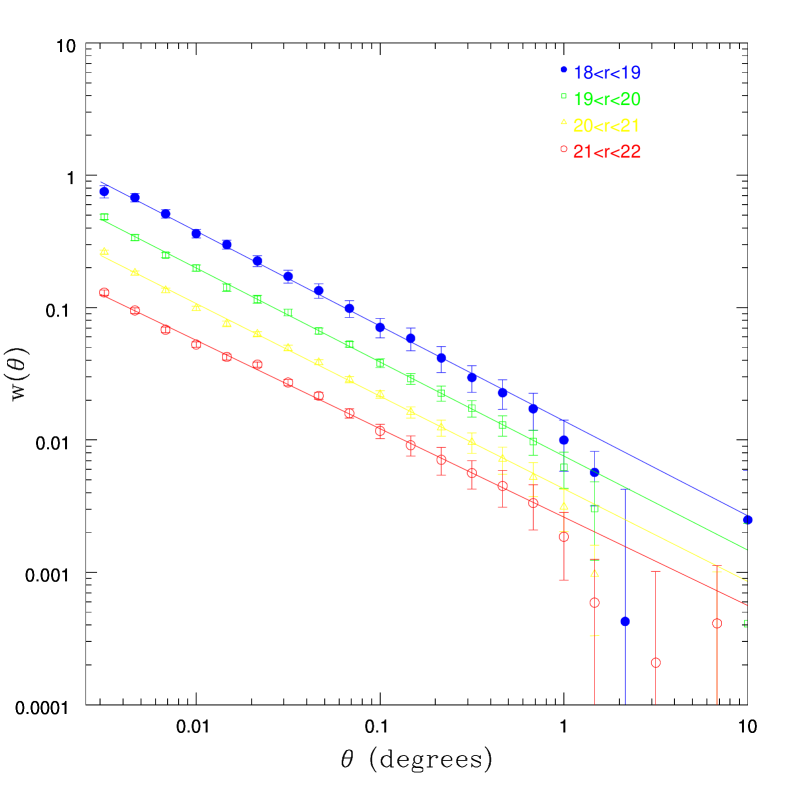
Figure 1: The angular correlation function $\omega(\theta)$ in different magnitude limited catalogs drawn from the SDSS database (from Connolly et al. 2002).

Previous measurements of $\omega(\theta)$, primarily from wide-field photographic plate surveys of the sky, have shown that $\omega(\theta)$ is rather well-fit (at least at small separations) by a power law: $\omega(\theta)=(\theta/\theta_{0})^{1-\gamma}$ with $\gamma\approx 1.7$. The clustering amplitude, characterized by $\theta_{0}$, is expected to depend on the depth of a magnitude limited survey such as the SDSS. This is because the galaxy distribution is expected to be clustered isotropically in three-dimensions. A photometric catalog projects out the radial component of the pair separation; the same angular separation can result from galaxies which have vastly different radial separations. Since the clustering amplitude is smaller on large separations, a deeper catalog contains more pairs which are close in the direction perpendicular to the line-of-sight but are well-separated along the line-of-sight, thus diluting the overall clustering signal.

Figure 1 shows $\omega(\theta)$ for SDSS galaxies in a number of different apparent magnitude bins. The solid lines show power-law fits to the data, over the range $1^{\prime}<\theta<30^{\prime}$ (the fits use the full covariance matrix from Scranton et al. 2002). Notice that the angular clustering signal on large scales is small: at one degree, $\omega(\theta)\sim 0.013$ for galaxies with $18<r^{*}<19$. Therefore, sky-position dependent errors in photometric calibration could dominate the signal. Scranton et al. (2002) describes the results of a battery of tests designed to quantify, and where possible correct for, the effects of photometric errors, stellar contamination, seeing, extinction, sky brightness, bright foreground objects and optical distortions in the camera itself. These tests highlight one of the great features of the SDSS dataset—its uniformity.

Notice that a power law is a good but not perfect description of the data. Also, the fainter catalogs, which contain galaxies out to greater distances, have a smaller angular clustering amplitude. The precise scaling with apparent magnitude depends on cosmology: a flat universe with $\Lambda=0.7$ provides a much cleaner scaling than does one in which $\Omega_{m}=1$ (but we have not shown this here). As a rough guide to the scales involved, note that the median redshift of galaxies with $18<r^{*}<19$ is $z_{m}=0.18$ (this median redshift is 0.24, 0.33 and 0.43 for the successively fainter galaxy catalogs). In a flat universe with $\Lambda=0.7$, one arcminute at $z=0.18$ corresponds to a distance of 154 $h^{-1}$kpc, so that 1 $h^{-1}$Mpc subtends about 0.11 degrees. Clearly, this estimate of $\omega(\theta)$ probes clustering on rather small scales. The next section describes an estimate of the clustering strength on larger scales.

2 The angular power spectrum $C_{\ell}$

There are three good reasons for computing the angular power spectrum $C_{\ell}$ in addition to the angular correlation function $\omega(\theta)$. First, on large scales, where the Gaussian approximation is most likely to apply, the $C_{\ell}$ estimators retain all of the information contained in the angular clustering signal. Therefore, they represent a lossless compression of the full data set. Second, although both $\omega(\theta)$ and $C_{\ell}$ are obtained by averaging the three dimensional power spectrum $P(k)$ over window functions, say $W_{\theta}(k)$ and $W_{\ell}(k)$, the second of these, $W_{\ell}$, is considerably narrower. This is advantageous if, as we will do shortly, one wishes to invert the measured two-dimensional statistic so as to constrain the form of $P(k)$. Narrow window functions are particularly important since small scale clustering is expected to be highly non-Gaussian; if the window function is broad, then one must worry about aliasing from small scale power. And third, it is possible to produce measurements of $C_{\ell}$ in which errors are uncorrelated.

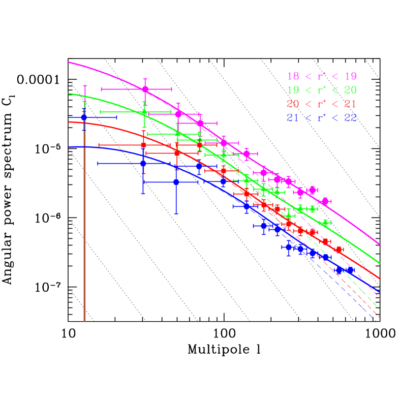
Figure 2: The angular power spectrum $C_{\ell}$ in different magnitude limited catalogs drawn from the SDSS database. As discussed in the text, a crude estimate of the underlying three dimensional power spectrum is obtained by shifting the same curve vertically and horizontally by an amount which depends on the survey depth: apparently fainter and more distant galaxies should be shifted farther up (because there is more averaging along the line-of-sight which has supressed fluctuations) and to the left (because as the survey depth increases a given angular scale $\ell$ corresponds to larger spatial scales). Dotted lines show the direction of this shift when the survey depth is changed (from Tegmark et al. 2002).

Briefly, the measurement is made by dividing the sky patch into $N$ square pixels each $12^{\prime}.5$ on a side and computing the density fluctuation $\delta_{i}=n_{i}/\bar{n}_{i}-1$ in each pixel. These $\delta_{i}$s can be grouped into a vector $d$, the covariance matrix of which is

$${\mbox{{\it\boldmath$C$}}}\equiv\Bigl{\langle}{\mbox{{\it\boldmath$d$}}}{\mbox{{\it\boldmath$d$}}^{\prime}}\Bigr{\rangle}={\mbox{{\it\boldmath$S$}}}+{\mbox{{\it\boldmath$N$}}}\qquad{\rm where}\qquad{\mbox{{\it\boldmath$S$}}}=\sum_{i}p_{i}{\mbox{{\it\boldmath$P$}}}_{i}.$$

Here $N$, assumed to be a diagonal matrix, denotes the contribution to $C$ which comes from the fact that the galaxy distribution is discrete (this is sometimes called the shot-noise contribution), and $p_{i}$ denotes the parameters which specify the amplitude of the power spectrum, and the ${\mbox{{\it\boldmath$P$}}}_{i}$ are matrices which are specified by the survey geometry in terms of Legendre polynomials.

The next step is to determine the $p_{i}$s from the observed data vector $d$. This involves repeatedly multiplying and inverting $N\times N$ matrices, which is computationally expensive. Therefore the Karhunen–Loève method is used to compress the information content of the map before estimating the power spectrum parameters. The actual estimates are made using a quadratic estimator which effectively Fourier transforms the sky map, squares the Fourier modes in the $i$th power spectrum band, and averages the results together. The details of this procedure are described in Tegmark et al. (2002).

The results are shown in Figure 2. A multipole $\ell$ corresponds roughly to an angular scale $\theta\sim 180^{\circ}/\ell$, so that $\ell=600$, for galaxies at $z=0.18$, corresponds roughly to a spatial scale of order 3 $h^{-1}$Mpc.

3 Inversion to the three-dimensional $P(k)$

The previous sections presented estimates of the angular correlation function and power spectrum from the SDSS database. These measurements can be used to derive constraints on the three dimensional power spectrum. This is possible because the angular power spectrum is related to the three dimensional power spectrum by

$$C_{\ell}=\int_{0}^{\infty}{dk\over k}\,k^{3}P(k)\,W_{\ell}(k),\qquad{\rm where}\qquad W_{\ell}(k)={2\over\pi}\left[\int_{0}^{\infty}dr\,f(r)\,j_{\ell}(kr)\right]^{2}.$$

Here $f$ is the probability distribution for the comoving distance $r$ to a random galaxy in the survey (which, in a photometric survey, is not measured), $j_{\ell}$ is a spherical Bessel function, and we have ignored the fact that the power spectrum evolves with redshift (strictly speaking, this expression also makes the standard assumption that clustering does not depend on luminosity; the next section shows that the data do not support this assumption, but the quantitative effect on the following analysis is small). To see what the definition above implies, note that for large values of $\ell$, corresponding to small angular scales, $j_{\ell}(kr)$ is sharply peaked around $kr=\ell$. Assuming the unknown $f(r)$ varies smoothly, we can set it equal to $f(\ell/k)$ and take it out of the integral above, leaving an integral over $j_{\ell}$ only which can be evaluated analytically. Thus, in this approximation, $\ell^{3}W_{\ell}(k)\to[(\ell/k)\,f(\ell/k)]^{2}$, and

$$C_{\ell}\to\int_{0}^{\infty}{dk\over k}\,{k^{3}P(k)\over\ell^{3}}\,\left[{\ell\over k}\,f\!\left({\ell\over k}\right)\right]^{2}\approx{k_{\ell}^{3}P(k_{\ell})\over\ell^{3}}\int_{0}^{\infty}{dk\over k}\,\left[{\ell\over k}\,f\!\left({\ell\over k}\right)\right]^{2},$$

where the second approximation comes from assuming that the term in square brackets is sharply peaked about its mean value $k_{\ell}$. This term depends on the distribution of comoving distances. To see how, define $r_{*}\equiv\int dr\,rf(r)$. Then the assumption that $f$ is peaked means we should set $r_{*}\equiv\beta\ell/k_{\ell}$, where $\beta$ is a constant of order unity. Thus, $C_{\ell}\approx(k_{\ell}/\ell)^{3}P(k_{\ell})\approx(\beta/r_{*})^{3}P(\beta\ell/r_{*})$. In other words, $C_{\ell}$ is a smoothed version of $P(k)$, which is shifted vertically (by a factor $r_{*}^{3}$) and horizontally (by $r_{*}$) on a log-log plot, by an amount which depends on the depth of the sample.

On small scales, the angular correlation function is also related to the power spectrum by a window function:

$$\omega(\theta)=\int{dk\over k}\,k^{2}P(k)\,W_{\theta}(k)\quad{\rm where}\quad W_{\theta}(k)={1\over 2\pi}\int dr\,J_{o}(kr\theta)\,f^{2}(r),$$

and $J_{o}$ is a Bessell function. In contrast to the window associated with $C_{\ell}$, this $W_{\theta}$ oscillates around zero, so that it is harder to associate a single wave number $k$ with the angular $\omega(\theta)$. Nevertheless, one can still develop techniques for inverting the measured $\omega(\theta)$ and $C_{\ell}$ to obtain the form of $P(k)$. A number of these methods are summarized in Dodelson et al. (2002).

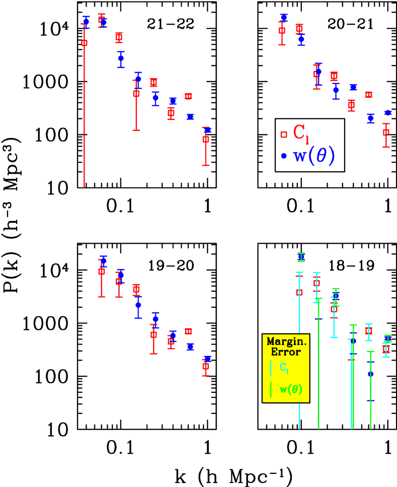
Figure 3: Comparison of $P(k)$ obtained by inverting $\omega(\theta)$ and $C_{\ell}$ in four apparent magnitude bins. Error bars are unmarginalized; marginalizing over the non-zero covariances between $k$ bins makes the error bars much larger (from Dodelson et al. 2002).

Clearly, the results of the inversion are sensitive to the assumed form for $f(r)$ which, in turn, depends on the magnitude limit of the sample and cosmology. (This is because, at fixed redshift, a flat model with $\Lambda>0$ has more volume than when $\Lambda=0$. Therefore, if the sample depth is characterized by a median redshift, which is observable at least in principle, then the typical physical separation between galaxies at that redshift is larger in a flat model with $\Lambda>0$.) Figure 3 shows the result of inverting $\omega(\theta)$ and $C_{\ell}$ in the four apparent magnitude limited samples presented earlier; the inversion assumed a flat model with $\Omega_{\Lambda}=0.7$. Over the range of scales where they overlap, the estimates agree with one another.

The implications for $P(k)$ are usually expressed as constraints on the parameters $\sigma_{8g}=b\sigma_{8}$ and $\Gamma$ which describe the amplitude (i.e. an up-down shift of all the points in Figure 3) and the shape (how far to the right does $P(k)$ peak). The subscript $g$ indicates that the measured $P(k)$ is of the galaxy distribution rather than the dark matter, and the factor $b$ comes from the standard assumption (consistent with numerical simulations of clustering on large scales) that the power in the two distributions differs only by a multiplicative linear bias factor. As the figure shows, the strongest constraints on the shape parameter come from the faintest galaxies (i.e. the magnitude bin $21<r<22$): $\Gamma=0.14^{+0.11}_{-0.06}$ ($95\%$ C.L.). The shape of $P(k)$ also depends on the baryon fraction $\Omega_{b}/\Omega_{m}$: increasing this ratio suppresses power on scales smaller than the peak, and analysis of the full data set will set interesting limits on this parameter also.

4 Direct estimates of $P(k)$

The previous subsection described estimates of the three dimensional $P(k)$ which were derived by first measuring projected quantities $\omega(\theta)$ and $C_{\ell}$. Since these are essentially smoothed versions of $P(k)$, an alternative procedure is to circumvent the initial measurement of projected quantities, and to work instead with quantities which optimize the signal-to-noise of the dataset. This is the KL approach taken by Szalay et al. (2002) who first expand the projected galaxy distribution on the sky over a set of Karhunen-Loève eigenfunctions, and then use a maximum likelihood analysis to derive constraints on the shape and amplitude of $P(k)$. For a flat universe with a cosmological constant, they find $\Gamma=0.188\pm 0.04$ and $\sigma_{8g}=0.915\pm 0.06$ (statistical errors only). Since $\Gamma\approx\Omega_{m}h$, if we use the HST measurement of the Hubble constant to set $h=0.7$, then the SDSS results imply $\Omega_{m}\approx 0.27$.

4 Clustering in $z$ space

The spectroscopic sample provides galaxy redshifts, and hence a reasonably accurate distance measurement, so that, in contrast to the angular photometric catalogs, a much stronger clustering signal can be measured. Moreover, because the redshift is available, it is possible to derive an accurate estimate of the intrinsic luminosity of each galaxy. This allows one to estimate how clustering depends on intrinsic, rather than apparent, properties of galaxies such as luminosity and rest-frame color. This is important because, in magnitude limited surveys like the SDSS, the most luminous galaxies are visible at the greatest distances, whereas the least luminous galaxies are only visible nearby. Therefore, the power on the largest scales is dominated by the clustering of the most luminous galaxies, whereas the power on smaller scales comes from a mix of galaxy types. If clustering depends on luminosity, then one must account for the changing mix of galaxy types at each scale when estimating the shape of the power spectrum.

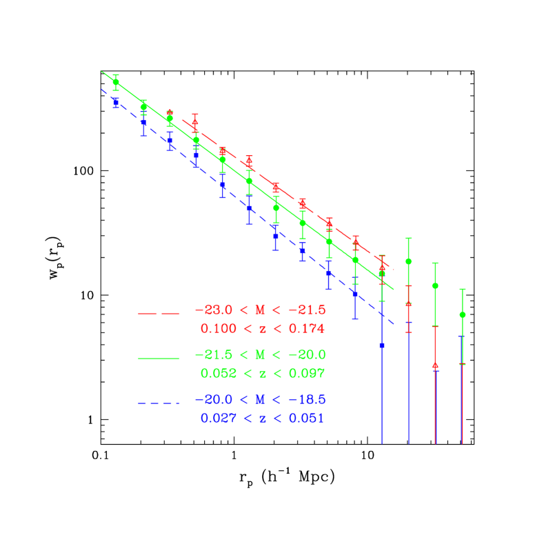
Figure 4: Galaxy clustering depends on luminosity. Changing the luminosity changes the amplitude but not the slope of the correlation function (from Zehavi et al. 2002).

As mentioned previously, peculiar velocities distort clustering statistics in redshift space. One way of accounting for these distortions is to measure the correlation function as a function of the separation parallel and perpendicular to the line-of-sight: $\xi_{2}(r_{p},\pi)$. Only separations parallel to the line-of-sight $\pi$ are affected by peculiar motions, so that

$$w_{p}(r_{p})\equiv 2\int_{0}^{\infty}d\pi\,\xi_{2}(r_{p},\pi)=2\int_{0}^{\infty}d\pi\,\xi\Bigl{(}\sqrt{r_{p}^{2}+\pi^{2}}\Bigr{)}$$

is independent of redshift-space distortions. Since

$$P(k_{p},k_{\pi})\equiv\int dr_{p}\int d\pi\,\xi_{2}(r_{p},\pi)\,\exp(-ik_{p}r_{p}-ik_{\pi}\pi),$$

the quantity $P(k_{p},0)$, being the Fourier transform of $w_{p}(r_{p})$, is also distortion free.

Measurements of the distortion-free correlation function and power spectrum both show that more luminous galaxies are more strongly clustered than less luminous galaxies (Figure 4). Whereas the amplitude of $\xi(r)$ appears to depend strongly on luminosity, the shape is approximately independent of $L$. On the other hand, the shape of the correlation function depends strongly on color: redder galaxies have steeper correlation functions (Figure 5).

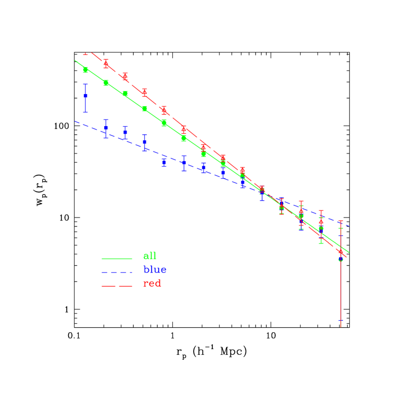
Figure 5: Galaxy clustering depends on color. Changing the color changes the slope and amplitude of $\xi(r)$ (from Zehavi et al. 2002).

As discussed by Budavari et al. (2003), these trends are qualitatively consistent with the following simple model. Suppose there are two types of galaxies, each with their own clustering pattern (say, a red population with a steeper correlation function than the blue population). Then the correlation function of the entire sample will be a weighted sum of the two populations, the weighting being determined by the relative numbers of the two types. Next, suppose that the amplitude of the correlation function in subsamples of each population depends on luminosity, and that the scaling with luminosity is similar for the two populations (on scales larger than 1 Mpc, this is a good description of the SDSS data; on smaller scales, clustering strength increases with luminosity for blue galaxies, whereas red galaxies show the opposite trend). Finally, suppose that the luminosity functions of these two populations have similar shapes, at least at the luminous end. These requirements guarantee that the correlation functions of subsamples defined by luminosity will always have the same shape, whereas subsamples defined differently will have different shapes. Explaining why this should be so is an interesting challenge for galaxy formation models.

A first study of clustering using photometric redshifts provides qualitatively similar results (Budavari et al. 2003). This is extremely encouraging because the use of photometric redshifts allows one to go considerably fainter than the spectroscopic dataset allows. In particular, photo-$z$s offer a cost-effective way of probing clustering out to redshifts of order unity. That this is possible at all is a tribute to the accuracy of the SDSS photometry.

Since the full $\xi(r_{p},\pi)$ is sensitive to peculiar velocities, whereas $w_{p}(r_{p})$ is not, a comparison of the two provides a measurement of galaxy peculiar velocities. On the small scales to which the present data is most sensitive, the dependence of clustering on luminosity and type constrains the velocity dispersions of the halos which different galaxy types populate. The SDSS data show that early-type galaxies populate halos with larger velocity dispersions (Zehavi et al. 2002), in qualitative agreement with the fact that such galaxies are much more common in massive clusters than in the field.

Since the first measurements of Totsuji & Kihara (1969), the galaxy correlation function has been characterized as a power law. A look through most of the figures presented here shows that, while a power law is indeed a good description, it is not perfect. The SDSS correlation functions show rich structure, much of which is statistically significant. In most ab initio models of $\xi(r)$, power-laws are purely fortuitous—they are not generic. Explaining the positions of the bumps and wiggles and their dependence on galaxy type, and hence extracting information from these features in $\xi(r)$ will become a rich area of research.

Funding for the creation and distribution of the SDSS Archive has been provided by the Alfred P. Sloan Foundation, the Participating Institutions, the National Aeronautics and Space Administration, the National Science Foundation, the U.S. Department of Energy, the Japanese Monbukagakusho, and the Max Planck Society. The SDSS Web site is http://www.sdss.org/.

References

- [1] Bahcall, N. A., Feng, D., Bode, P., et al. 2002, ApJ, in press (astro-ph/0205490)
- [2] Budavari, T., Connolly, A. J., Szalay, A. S., et al. 2003 (in preparation)
- [3] Connolly, A. J., Scranton, R., Johnston, D., et al. 2002, ApJ, 579, 42
- [4] Dodelson, S., Narayanan, V. K., Tegmark, M., et al. 2002, ApJ, 572, 140
- [5] Fukugita, M., Ichikawa, T., Gunn, J. E., et al. 1996, AJ, 111, 1748
- [6] Gunn, J.E., Carr, M.A., Rockosi, C.M., Sekiguchi, M., et al. 1998, AJ, 116, 3040
- [7] Hoyle, F., Vogeley, M. S., Gott III, J. R. 2002, ApJ, 580, 663
- [8] McKay, T. A., Sheldon, E. S., Racusin, J., et al. 2002, ApJ, submitted (astro-ph/0108013)
- [9] Nichol, R., Miller, C., Connolly, A., et al. 2000, HEAD meeting 32, 14.02 (astro-ph/0011557)
- [10] Scranton, R., Johnston, D., Dodelson, S., et al. 2002, ApJ, 579, 48
- [11] Stoughton, C., Lupton, R.H., Bernardi, M., et al. 2002, AJ, 123, 485 (Early Data Release)
- [12] Strauss, M.A., Weinberg, D.H., Lupton, R.H. et al. 2002, AJ, 124, 1810
- [13] Szalay, A. S., Jain, B., Matsubara, T., et al. 2002, ApJ, in press (astro-ph/0107419)
- [14] Szapudi, I., Frieman, J. A., Scoccimarro, R. 2002, ApJ, 570, 75
- [15] Tegmark, M., Dodelson, S., Eisenstein, D. J., et al. 2002, ApJ, 571, 191
- [16] Totsuji, H. & Kihara, T. 1969, PASJ, 21, 221
- [17] York, D.G., Adelman, J., Anderson, J.E., et al. 2000, AJ, 120, 1579
- [18] Zehavi, I., Blanton, M., Frieman, J., et al. 2002, ApJ, 571, 172