New Orbits for the $n$-Body Problem

Abstract

In this paper, we consider minimizing the action functional as a method for numerically discovering periodic solutions to the $n$-body problem. With this method, we can find a large number of choreographies and other more general solutions. We show that most of the solutions found, including all but one of the choreographies, are unstable. It appears to be much easier to find unstable solutions to the $n$-body problem than stable ones. Simpler solutions are more likely to be stable than exotic ones.

1 Least Action Principle

Given $n$ bodies, let $m_{j}$ denote the mass and $z_{j}(t)$ denote the position in ${\mathbb{R}}^{2}={\mathbb{C}}$ of body $j$ at time $t$. The action functional is a mapping from the space of all trajectories, $z_{1}(t),z_{2}(t),\ldots,z_{n}(t)$, $0\leq t\leq 2\pi$, into the reals. It is defined as the integral over one period of the kinetic minus the potential energy:

$$A=\int_{0}^{2\pi}\left(\sum_{j}\frac{m_{j}}{2}\|\dot{z}_{j}\|^{2}+\sum_{j,k:k<j}\frac{m_{j}m_{k}}{\|z_{j}-z_{k}\|}\right)dt.$$

Stationary points of the action function are trajectories that satisfy the equations of motions, i.e., Newton’s law gravity. To see this, we compute the first variation of the action functional,

$$\delta A = \int_{0}^{2\pi}\sum_{\alpha}\left(\sum_{j}m_{j}\dot{z}_{j}^{\alpha}\dot{\delta z}_{j}^{\alpha}-\sum_{j,k:k<j}m_{j}m_{k}\frac{(z_{j}^{\alpha}-z_{k}^{\alpha})(\delta z_{j}^{\alpha}-\delta z_{k}^{\alpha})}{\|z_{j}-z_{k}\|^{3}}\right)dt$$

$$= -\int_{0}^{2\pi}\sum_{j}\sum_{\alpha}\left(m_{j}\ddot{z}_{j}^{\alpha}+\sum_{k:k\neq j}m_{j}m_{k}\frac{z_{j}^{\alpha}-z_{k}^{\alpha}}{\|z_{j}-z_{k}\|^{3}}\right)\delta z_{j}^{\alpha}dt,$$

and set it to zero. We get that

$$m_{j}\ddot{z}_{j}^{\alpha}=-\sum_{k:k\neq j}m_{j}m_{k}\frac{z_{j}^{\alpha}-z_{k}^{\alpha}}{\|z_{j}-z_{k}\|^{3}},\qquad j=1,2,\ldots,n,\quad\alpha=1,2$$ (1)

Note that if $m_{j}=0$ for some $j$, then the first order optimality condition reduces to $0=0$, which is not the equation of motion for a massless body. Hence, we must assume that all bodies have strictly positive mass.

2 Periodic Solutions

Our goal is to use numerical optimization to minimize the action functional and thereby find periodic solutions to the $n$-body problem. Since we are interested only in periodic solutions, we express all trajectories in terms of their Fourier series:

$$z_{j}(t)=\sum_{k=-\infty}^{\infty}\gamma_{k}e^{ikt},\qquad\gamma_{k}\in{\mathbb{C}}.$$

Abandoning the efficiency of complex-variable notation, we can write the trajectories with components $z_{j}(t)=(x_{j}(t),y_{j}(t))$ and $\gamma_{k}=(\alpha_{k},\beta_{k}).$ So doing, we get

$$x(t) = a_{0}+\sum_{k=1}^{\infty}\left(a_{k}^{c}\cos(kt)+a_{k}^{s}\sin(kt)\right)$$

$$y(t) = b_{0}+\sum_{k=1}^{\infty}\left(b_{k}^{c}\cos(kt)+b_{k}^{s}\sin(kt)\right)$$

where

$$a_{0}=\alpha_{0},\qquad a_{k}^{c} = \alpha_{k}+\alpha_{-k},\qquad a_{k}^{s}=\beta_{-k}-\beta_{k},$$

$$b_{0}=\beta_{0},\qquad b_{k}^{c} = \beta_{k}+\beta_{-k},\qquad b_{k}^{s}=\alpha_{k}-\alpha_{-k}.$$

Since we plan to optimize over the space of trajectories, the parameters $a_{0}$, $a_{k}^{c}$, $a_{k}^{s}$, $b_{0}$, $b_{k}^{c}$, and $b_{k}^{s}$ are the decision variables in our optimization model. The objective is to minimize the action functional.

ampl is a small programming language designed for the efficient expression of optimization problems Fourer et al. (1993). Figure 1 shows the ampl program for minimizing the action functional.

Note that the action functional is a nonconvex nonlinear functional. Hence, it is expected to have many local extrema and saddle points. We use the author’s local optimization software called loqo (see Vanderbei (1999), Vanderbei and Shanno (1999)) to find local minima in a neighborhood of an arbitrary given starting trajectory. One can provide either specific initial trajectories or one can give random initial trajectories. The four lines just before the call to solve in Figure 1 show how to specify a random initial trajectory. Of course, ampl provides capabilities of printing answers in any format either on the standard output device or to a file. For the sake of brevity and clarity, the print statements are not shown in Figure 1. ampl also provides the capability to loop over sections of code. This is also not shown but the program we used has a loop around the four initialization statements, the call to solve the problem, and the associated print statements. In this way, the program can be run once to solve for a large number of periodic solutions.

2.1 Choreographies

Recently, Chenciner and Montgomery (2000) introduced a new family of solutions to the $n$-body problem called choreographies. A choreography is defined as a solution to the $n$-body problem in which all of the bodies share a common orbit and are uniformly spread out around this orbit. Such trajectories are even easier to find using the action principle. Rather than having a Fourier series for each orbit, it is only necessary to have one master Fourier series and to write the action functional in terms of it. Figure 2 shows the ampl model for finding choreographies.

3 Stable vs. Unstable Solutions

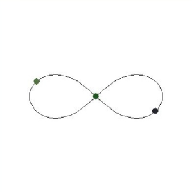
FigureEight3

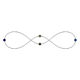
Braid4

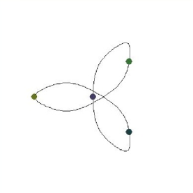
Trefoil4

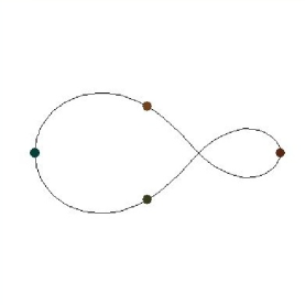
FigureEight4

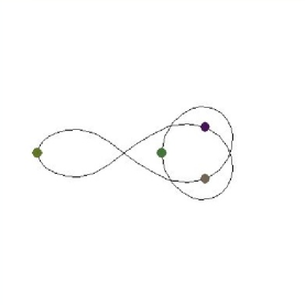
FoldedTriLoop4

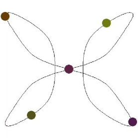
Trefoil5

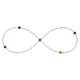
FigureEight5

Figure 3: Periodic Orbits—Choreographies.

Figure 3 shows some simple choreographies found by minimizing the action functional using the ampl model in Figure 2. The famous $3$-body figure eight, first discoverd by Moore (1993) and later analyzed by Chenciner and Montgomery (2000), is the first one shown—labeled FigureEight3. It is easy to find choreographies of arbitrary complexity. In fact, it is not hard to rediscover most of the choreographies given in Chenciner et al. (2001), and more, simply by putting a loop in the ampl model and finding various local minima by using different starting points.

However, as we discuss in a later section, simulation makes it apparent that, with the sole exception of FigureEight3, all of the choreographies we found are unstable. And, the more intricate the choreography, the more unstable it is. Since the only choreographies that have a chance to occur in the real world are stable ones, many cpu hours were devoted to searching for other stable choreographies. So far, none have been found. The choreographies shown in Figure 3 represent the ones closest to being stable.

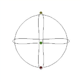
Ducati3

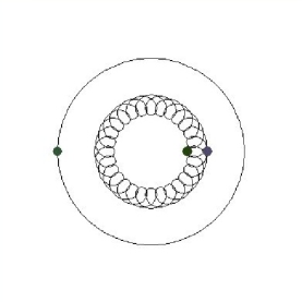
Hill3_15

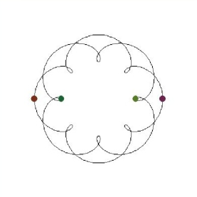
DoubleDouble5

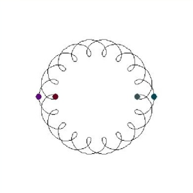
DoubleDouble10

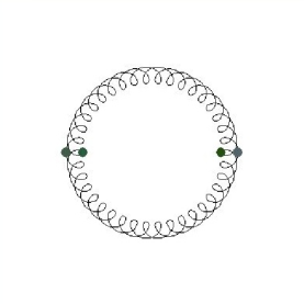
DoubleDouble20

OrthQuasiEllipse4

Rosette4

PlateSaucer4

BorderCollie4

Figure 4: Periodic Orbits–Non-Choreographies.

Given the difficulty of finding stable choreographies, it seems interesting to search for stable nonchoreographic solutions using, for example, the ampl model from Figure 1. The most interesting such solutions are shown in Figure 4. The one labeled Ducati3 is stable as are Hill3_15 and the three DoubleDouble solutions. However, the more exotic solutions (OrthQuasiEllipse4, Rosette4, PlateSaucer4, and BorderCollie4) are all unstable.

For the interested reader, a java applet can be found at Vanderbei (2001) that allows one to watch the dynamics of each of the systems presented in this paper (and others). This applet actually integrates the equations of motion. If the orbit is unstable it becomes very obvious as the bodies deviate from their predicted paths.

3.1 Ducati3 and its Relatives

The Ducati3 orbit first appeared in Moore (1993) and has been independently rediscovered by this author, Broucke Broucke (2003), and perhaps others. Simulation reveals it to be a stable system. The java applet at Vanderbei (2001) allows one to rotate the reference frame as desired. By setting the rotation to counter the outer body in Ducati3, one discovers that the other two bodies are orbiting each other in nearly circular orbits. In other words, the first body in Ducati3 is executing approximately a circular orbit, $z_{1}(t)=-e^{it}$, the second body is oscillating back and forth roughly along the $x$-axis, $z_{2}(t)=\cos(t)$, and the third body is oscillating up and down the $y$-axis, $z_{3}(t)=i\sin(t)$. Rotating so as to fix the first body means multiplying by $e^{-it}$:

$$\bar{z}_{1}(t) = e^{-it}(-e^{it})=-1$$

$$\bar{z}_{2}(t) = e^{-it}\cos(t)=(1+e^{-2it})/2$$

$$\bar{z}_{2}(t) = e^{-it}i\sin(t)=(1-e^{-2it})/2.$$

Now it is clear that bodies 2 and 3 are orbiting each other at half the distance of body 1. So, this system can be described as a Sun, Earth, Moon system in which all three bodies have equal mass and in which one (sidereal) month equals one year. The synodic month is shorter—half a year.

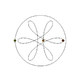
Hill3_2

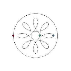
Hill3_3

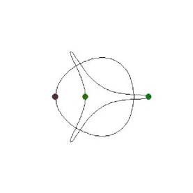
Hill3_0.5

Figure 6: Periodic Orbits—Hill-type with equal masses.

This analysis of Ducati3 suggests looking for other stable solutions of the same type but with different resonances between the length of a month and a year. Hill3_15 is one of many such examples we found. In Hill3_15, there are 15 sidereal months per year. Let Hill3_$n$ denote the system in which there are $n$ months in a year. All of these orbits are easy to calculate and they all appear to be stable. This success suggests going in the other direction. Let Hill3_$\frac{1}{n}$ denote the system in which there are $n$ years per month. We computed Hill3_$\frac{1}{2}$ and found it to be unstable. It is shown in Figure 6.

In the preceding discussion, we decomposed these Hill-type systems into two $2$-body problems: the Earth and Moon orbit each other while their center of mass orbits the Sun. This suggests that we can find stable orbits for the $4$-body problem by splitting the Sun into a binary star. This works. The orbits labeled DoubleDouble$n$ are of this type. As already mentioned, these orbits are stable.

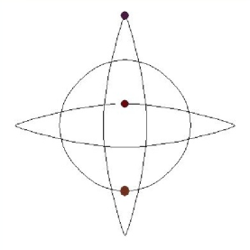
Ducati3_2

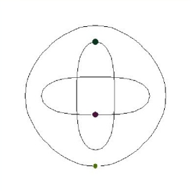
Ducati3_0.5

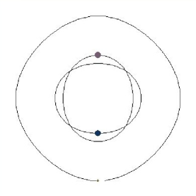
Ducati3_0.1

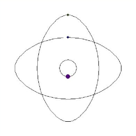
Ducati3_10

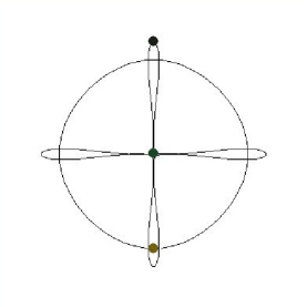
Ducati3_1.2

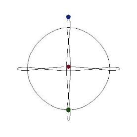
Ducati3_1.3

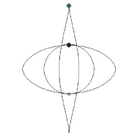
Ducati3_alluneq

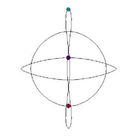
Ducati3_alluneq2

Figure 5: Periodic Orbits—Ducati’s with unequal masses.

Given the existence and stability of FigureEight3, one often is asked if there is any chance to observe such a system among the stars. The answer is that it is very unlikely since its existence depends crucially on the masses being equal. The Ducati and Hill type orbits, however, are not constrained to have their masses be equal. Figure 5 shows several Ducati-type orbits in which the masses are not all equal. All of these orbits are stable. This suggests that stability is common for Ducati and Hill type orbits. Perhaps such orbits can be observed.

4 Limitations of the Model

The are certain limitations to the approach articulated above. First, the Fourier series is an infinite sum that gets truncated to a finite sum in the computer model. Hence, the trajectory space from which solutions are found is finite dimensional.

Second, the integration is replaced with a Riemann sum. If the discretization is too coarse, the solution found might not correspond to a real solution to the $n$-body problem. The only way to be sure is to run a simulator.

Third, as mentioned before, all masses must be positive. If there is a zero mass, then the stationary points for the action function, which satisfy (1), don’t necessarily satisfy the equations of motion given by Newton’s law.

Lastly, the model, as given in Figure 1, can’t solve 2-body problems with eccentricity. We address this issue in the next section.

5 Elliptic Solutions

An ellipse with semimajor axis $a$, semiminor axis $b$, and having its left focus at the origin of the coordinate system is given parametrically by:

$$x(t)=f+a\cos t,\qquad y(t)=b\sin t,$$

where $f=\sqrt{a^{2}-b^{2}}$ is the distance from the focus to the center of the ellipse.

However, this is not the trajectory of a mass in the $2$-body problem. Such a mass will travel faster around one focus than around the other. To accomodate this, we need to introduce a time-change function $\theta(t)$:

$$x(t)=f+a\cos\theta(t),\qquad y(t)=b\sin\theta(t).$$

This function $\theta$ must be increasing and must satisfy $\theta(0)=0$ and $\theta(2\pi)=2\pi$.

The optimization model can be used to find (a discretization of) $\theta(t)$ automatically by changing param theta to var theta and adding appropriate monotonicity and boundary constraints. In this manner, more realistic orbits can be found that could be useful in real space missions.

In particular, using an eccentricity $e=f/a=0.0167$ and appropriate Sun and Earth masses, we can find a periodic Hill-Type satellite trajectory in which the satellite orbits the Earth once per year.

6 Sensitivity Analysis

The determination of stability vs. instability mentioned the previous sections was done empirically by simulating the orbits with a integrator and very small step sizes. Two integrators were used: a midpoint integrator and a $4$-th order Runge-Kutta integrator. Orbits that are claimed to be stable were run for several hours of cpu time (which corresponds to many thousands of orbits) without falling apart. Orbits that are claimed to be unstable generally became obviously so in just a few seconds of cpu time, which corresponds to only a few full orbits. In this section, we describe a Floquet analysis of stability and present this measure of stability for the various orbits found.

For simplicity, in this section we assume that all masses are equal to one. Let $\xi^{*}(t)=(z^{*}(t),\dot{z}^{*}(t))$ be a particular solution to

$$\dot{\xi}=A(\xi)$$

where

$$A\left(z(t),\dot{z}(t)\right)=(\dot{z}(t),a(z(t)))$$

and

$$a(z)=(a_{1}(z),\ldots,a_{n}(z))$$

and

$$a_{j}(z)=-\sum_{k:k\neq j}\frac{z_{j}-z_{k}}{\|z_{j}-z_{k}\|^{2}},\quad j=1,2,\ldots,n.$$

Consider a nearby solution $\xi(t)$:

$$\dot{\xi}(t) = A(\xi(t))$$

$$\approx A(\xi^{*}(t))+A^{\prime}(\xi^{*}(t))(\xi(t)-\xi^{*}(t))$$

$$= \dot{\xi}^{*}(t)+A^{\prime}(\xi^{*}(t))(\xi(t)-\xi^{*}(t)).$$

Put $\Delta\xi=\xi-\xi^{*}$. Then $\dot{\Delta\xi}=A^{\prime}(\xi^{*}(t))\Delta\xi.$ A finite difference approximation yields

$$\Delta\xi(t+h) = \Delta\xi(t)+hA^{\prime}(\xi^{*}(t))\Delta\xi(t)$$

$$= \left(I+hA^{\prime}(\xi^{*}(t))\right)\Delta\xi(t).$$

Iterating around one period, we get:

$$\Delta\xi(T)=\left(\prod_{i=0}^{n-1}\left(I+hA^{\prime}(\xi^{*}(t_{i}))\right)\right)\Delta\xi(0),$$

where $h=T/n$ and $t_{i}=iT/n$.

The following perturbations, which are associated with invariants of the physical laws, are unimportant in calculating $\Delta\xi(T)$:

$$\left[\begin{array}[]{c}\Delta z\\ \Delta\dot{z}\end{array}\right]=\left[\begin{array}[]{c}e_{1}\\ e_{1}\\ e_{1}\\ 0\\ 0\\ 0\end{array}\right],\quad\left[\begin{array}[]{c}e_{2}\\ e_{2}\\ e_{2}\\ 0\\ 0\\ 0\end{array}\right],\quad\left[\begin{array}[]{c}0\\ 0\\ 0\\ e_{1}\\ e_{1}\\ e_{1}\end{array}\right],\quad\left[\begin{array}[]{c}0\\ 0\\ 0\\ e_{2}\\ e_{2}\\ e_{2}\end{array}\right],\quad\left[\begin{array}[]{c}Rz_{1}\\ Rz_{2}\\ Rz_{3}\\ R\dot{z}_{1}\\ R\dot{z}_{2}\\ R\dot{z}_{3}\end{array}\right],\quad\frac{1}{2}\left[\begin{array}[]{c}-3\dot{z}_{1}+2z_{1}\\ -3\dot{z}_{1}+2z_{1}\\ -3\dot{z}_{1}+2z_{1}\\ -3a_{1}-\dot{z}_{1}\\ -3a_{2}-\dot{z}_{2}\\ -3a_{3}-\dot{z}_{3}\end{array}\right],$$

where $R$ denotes rotation by $90^{\circ}$. The first two of these perturbations correspond to translation. The next two correspond to moving frame of reference and the last two correspond to rotation, and dilation. Dilation is explained below. Of course, all positions and velocities are evaluated at $t=0$. Vector $e_{i}$ denotes the $i$-th unit vector in ${\mathbb{R}}^{2}$.

Consider spatial dilation by $\rho$ together with a temporal dilation by $\theta$:

$$Z_{j}(t)=\rho z_{j}(t/\theta).$$

Given that the $z_{j}$’s are a solution, it is easy to check that

$$\ddot{Z}_{j}(t)=-\frac{\rho^{3}}{\theta^{2}}\sum_{k\neq j}\frac{Z_{j}(t)-Z_{k}(t)}{\|Z_{j}(t)-Z_{k}(t)\|^{2}}.$$

Hence, if mass is to remain fixed, we must have that $\rho^{3}=\theta^{2}$:

$$Z_{j}(t)=\rho z_{j}(t/\rho^{3/2})\qquad\dot{Z}_{j}(t)=\rho^{-1/2}\dot{z}_{j}(t/\rho^{3/2}).$$

To find the perturbation direction corresponding to this dilation, we differentiate with respect to $\rho$ at $\rho=1$:

$$\frac{d}{d\rho}\left.\left[\begin{array}[]{c}\rho z_{j}(t/\rho^{3/2})\\ \rho^{-1/2}\dot{z}_{j}(t/\rho^{3/2})\end{array}\right]\right|_{\rho=1}=\left[\begin{array}[]{c}-\frac{3}{2}\dot{z}_{j}+z_{j}\\ -\frac{3}{2}a_{j}-\frac{1}{2}\dot{z}_{j}\end{array}\right].$$

For checking stability, we project any initial perturbation onto the null space of $P^{T}$, where

$$P=\left[\begin{array}[]{cccccc}e_{1}&e_{2}&0&0&Rz_{1}&(-3\dot{z}_{1}+2z_{1})/2\\ e_{1}&e_{2}&0&0&Rz_{2}&(-3\dot{z}_{2}+2z_{2})/2\\ e_{1}&e_{2}&0&0&Rz_{3}&(-3\dot{z}_{3}+2z_{3})/2\\ 0&0&e_{1}&e_{2}&R\dot{z}_{1}&(-3a_{1}-\dot{z}_{1})/2\\ 0&0&e_{1}&e_{2}&R\dot{z}_{2}&(-3a_{2}-\dot{z}_{2})/2\\ 0&0&e_{1}&e_{2}&R\dot{z}_{3}&(-3a_{3}-\dot{z}_{3})/2\end{array}\right].$$

The projection matrix is given by

$$\Pi=I-P(P^{T}P)^{-1}P^{T}.$$

From the fact that $z_{1}+z_{2}+z_{3}=0$ and $\dot{z}_{1}+\dot{z}_{2}+\dot{z}_{3}=0$, it follows that all columns of $P$ are mutually orthogonal except for the 5-th and 6-th columns. Hence, $P^{T}P$ is not a purely diagonal matrix.

Let

$$\Lambda_{n}=\left(\prod_{i=0}^{n-1}\left(I+hA^{\prime}(\xi^{*}(t_{i}))\right)\right).$$

We say that an orbit is stable if all eigenvalues of

$$\lim_{n\rightarrow\infty}\Lambda_{n}\Pi$$

are at most one in magnitude.

6.1 Stable Orbits

We computed $\Lambda_{n}$ for $n=10^{6}$. Table 1 shows maximum eigenvalues for those orbits that seemed stable from simulation. Table 2 shows maximum eigenvalues for those orbits that appeared unstable when simulated.

Acknowledgements. The author received support from the NSF (CCR-0098040) and the ONR (N00014-98-1-0036).

Name	$\max(\lambda_{i}(\Lambda))$	$\max(\lambda_{i}(\Lambda\Pi))$
Lagrange2	1.383	1.362
FigureEight3	1.228	4.220
Ducati3	1.105	3.885
Hill3_15	1.444	2.403
DoubleDouble5	12.298	12.298
DoubleDouble10	1.404	5.948
DoubleDouble20	1.890	1.890

Table 1: Apparently stable orbits.

Name	$\max(\lambda_{i}(\Lambda))$	$\max(\lambda_{i}(\Lambda\Pi))$
Lagrange3	81.630	81.630
OrthQuasiEllipse4	18.343	18.343
Rosette4	1.873	4.449
Braid4	727.508	711.811
Trefoil4	41228.515	41213.852
FigureEight4	221.642	194.095
FoldedTriLoop4	74758.355	74675.092
PlateSaucer4	3653.210	3653.210
BorderCollie4	188.235	188.052
Trefoil5	1.913e+8	1.917e+8
FigureEight5	2223.137	2223.457

Table 2: Apparently unstable orbits.

param N := 3;  # number of masses
param n := 15;  # number of terms in Fourier series representation
param m := 100;  # number of terms in numerical approx to integral

set Bodies := {0..N-1};
set Times  := {0..m-1} circular; # "circular" means that next(m-1) = 0

param theta {t in Times} := t*2*pi/m;
param dt := 2*pi/m;

param a0 {i in Bodies} default 0;        param b0 {i in Bodies} default 0;
var as {i in Bodies, k in 1..n} := 0;    var bs {i in Bodies, k in 1..n} := 0;
var ac {i in Bodies, k in 1..n} := 0;    var bc {i in Bodies, k in 1..n} := 0;

var x {i in Bodies, t in Times}
  = a0[i]+sum {k in 1..n} ( as[i,k]*sin(k*theta[t]) + ac[i,k]*cos(k*theta[t]) );
var y {i in Bodies, t in Times}
  = b0[i]+sum {k in 1..n} ( bs[i,k]*sin(k*theta[t]) + bc[i,k]*cos(k*theta[t]) );

var xdot {i in Bodies, t in Times} = (x[i,next(t)]-x[i,t])/dt;
var ydot {i in Bodies, t in Times} = (y[i,next(t)]-y[i,t])/dt;

var K {t in Times} = 0.5*sum {i in Bodies} (xdot[i,t]^2 + ydot[i,t]^2);

var P {t in Times}
  = - sum {i in Bodies, ii in Bodies: ii>i}
            1/sqrt((x[i,t]-x[ii,t])^2 + (y[i,t]-y[ii,t])^2);

minimize A: sum {t in Times} (K[t] - P[t])*dt;

let {i in Bodies, k in 1..n} as[i,k] := 1*(Uniform01()-0.5);
let {i in Bodies, k in 1..n} ac[i,k] := 1*(Uniform01()-0.5);
let {i in Bodies, k in n..n} bs[i,k] := 0.01*(Uniform01()-0.5);
let {i in Bodies, k in n..n} bc[i,k] := 0.01*(Uniform01()-0.5);

solve;

Figure 1: ampl program for finding trajectories that minimize the action functional.

param N := 3;  # number of masses
param n := 15;  # number of terms in Fourier series representation
param m := 99;  # terms in num approx to integral.  must be a multiple of N

param lagTime := m/N;

set Bodies := {0..N-1};
set Times  := {0..m-1} circular; # "circular" means that next(m-1) = 0

param theta {t in Times} := t*2*pi/m;
param dt := 2*pi/m;

param a0 default 0;         param b0 default 0;
var as {k in 1..n} := 0;    var bs {k in 1..n} := 0;
var ac {k in 1..n} := 0;    var bc {k in 1..n} := 0;

var x {i in Bodies, t in Times}
  = a0+sum {k in 1..n} ( as[k]*sin(k*theta[(t+i*lagTime) mod m])
                       + ac[k]*cos(k*theta[(t+i*lagTime) mod m]) );
var y {i in Bodies, t in Times}
  = b0+sum {k in 1..n} ( bs[k]*sin(k*theta[(t+i*lagTime) mod m])
                       + bc[k]*cos(k*theta[(t+i*lagTime) mod m]) );

var xdot {i in Bodies, t in Times} = (x[i,next(t)]-x[i,t])/dt;
var ydot {i in Bodies, t in Times} = (y[i,next(t)]-y[i,t])/dt;

var K {t in Times} = 0.5*sum {i in Bodies} (xdot[i,t]^2 + ydot[i,t]^2);

var P {t in Times}
  = - sum {i in Bodies, ii in Bodies: ii>i}
            1/sqrt((x[i,t]-x[ii,t])^2 + (y[i,t]-y[ii,t])^2);

minimize A: sum {t in Times} (K[t] - P[t])*dt;

let {k in 1..n} as[k] := 1*(Uniform01()-0.5);
let {k in 1..n} ac[k] := 1*(Uniform01()-0.5);
let {k in n..n} bs[k] := 0.01*(Uniform01()-0.5);
let {k in n..n} bc[k] := 0.01*(Uniform01()-0.5);

solve;

Figure 2: ampl program for finding choreographies by minimizing the action functional.

References

- Broucke (2003) R. Broucke. New orbits for the -body problem. In Proceedings of Conference on New Trends in Astrodynamics and Applications, 2003.
- Chenciner et al. (2001) A. Chenciner, J. Gerver, R. Montgomery, and C. Simó. Simple choreographic motions on bodies: a preliminary study. In Geometry, Mechanics and Dynamics, 2001.
- Chenciner and Montgomery (2000) A. Chenciner and R. Montgomery. A remarkable periodic solution of the three-body problem in the case of equal masses. Annals of Math, 152:881–901, 2000.
- Fourer et al. (1993) R. Fourer, D.M. Gay, and B.W. Kernighan. AMPL: A Modeling Language for Mathematical Programming. Scientific Press, 1993.
- Moore (1993) C. Moore. Braids in classical gravity. Phys. Rev. Lett., 70:3675–3679, 1993.
- Vanderbei (1999) R.J. Vanderbei. LOQO user’s manual—version 3.10. Optimization Methods and Software, 12:485–514, 1999.
- Vanderbei (2001) R.J. Vanderbei. http://www.princeton.edu/rvdb/JAVA/astro/galaxy/Galaxy.html, 2001. .
- Vanderbei and Shanno (1999) R.J. Vanderbei and D.F. Shanno. An interior-point algorithm for nonconvex nonlinear programming. Computational Optimization and Applications, 13:231–252, 1999.