Interacting quintessence solution to the coincidence problem
Abstract
We show that a suitable interaction between a scalar field and a matter fluid in a spatially homogeneous and isotropic spacetime can drive the transition from a matter dominated era to an accelerated expansion phase and simultaneously solve the coincidence problem of our present Universe. For this purpose we study the evolution of the energy density ratio of these two components. We demonstrate that a stationary attractor solution is compatible with an accelerated expansion of the Universe. We extend this study to account for dissipation effects due to interactions in the dark matter fluid. Finally, Type Ia supernovae and primordial nucleosynthesis data are used to constrain the parameters of the model.
pacs:
98.80.Hw, 04.20.JbI Introduction
Nowadays there is a wide consensus among observational cosmologists that our Universe is accelerating its expansion -for a pedagogical short update see pedagogical , see also Perlmutter98 ; Riess98 ; paris ; Efstat ; Perlmutter99 ; Bahcall99 ; Efstat02 - which implies that the Einstein-de Sitter scenario has to be abandoned, at least to describe the present era. The nature of the dark energy behind this acceleration is unknown. Two main proposals, namely the CDM model and QCDM models have been advanced. The former assumes a cosmological constant arising from the energy density of the zero point fluctuations of the quantum vacuum and cold dark matter in the form of pressureless dust. While it fits rather well all the observational constraints melchiorri it has serious difficulties with the low observed value of this vacuum energy (that by all accounts should be many orders of magnitude higher) and fails to address the so–called “coincidence problem”, namely why the energy density of both components happen to be of the same order today? The second group of models assume an evolving scalar field possessing a negative pressure and cold dark matter. It also fits well the observational constraints, and seems rather natural but it is not clear whether it really solves the coincidence problem (for a recent review see paris ).
Most of the QCDM models assume that the dark matter and the scalar field components evolve independently. However, given that the physical nature of the quintessence field is still unknown and also that the dark matter may well be a substratum not as simple as a pressureless perfect fluid, there seems to be no a priori reasons to exclude a coupling between both components. Interacting quintessence models have been shown to provide qualitatively new features which may be relevant to the coincidence problem luca ; zpc . In particular, it has been demonstrated that a suitable coupling may give rise to a stable constant ratio of the energy densities of both components which is compatible with an accelerated expansion of the Universe zpc . On the other hand, this model could not answer the question of how such a stationary solution can be obtained as the result of a dynamical evolution. In the present paper we clarify this point and establish an exactly solvable model for a smooth transition from a matter dominated phase to a subsequent period of accelerated expansion. This model implies the evolution of the density ratio towards a finite, stable, asymptotic value. Thus it may represent a solution to the coincidence problem.
As shown in another previous paper, a very suitable ingredient of quintessence models is a dissipative, negative, scalar pressure of the matter component. Such a quantity may simultaneously help to drive acceleration and solve the coincidence problem enlarged . A negative pressure arises naturally from bulk viscous dissipation, quantum particle production or self-interaction in the matter component antf . Here we combine the advantages of quintessence models interacting with matter (QIM) with those relying on a dissipative pressure within the latter.
The aim of this paper is to show, that on this basis a solution of the coincidence problem in an accelerating universe can be realized in a comparatively simple manner within the framework of general relativity.
The paper is organized as follows. Section II introduces the basic equations of the model. Section III explores the dynamics of the energy density ratio, including the stability properties of the stationary solutions. Furthermore, it derives the corresponding scalar field potential. Section IV investigates the role of a dissipative pressure within the dark matter component and discusses the behavior of the deceleration parameter. In section V the available magnitude–redshift data of supernovae Type Ia (SNe Ia) are used in combination with primordial nucleosynthesis data to restrict the parameters of the model. Section VI presents our conclusions and final comments. Lastly, the Appendix discusses briefly the connections of the matter-quintessence coupling with cosmological inhomogeneities, the issue of possible anomalous acceleration of baryonic matter and some consequences of this interaction on the early universe. Units have been chosen so that .
II Interacting cosmology
Let us assume a FLRW spacetime with matter and a minimally coupled scalar field. The Friedmann equation and the overall conservation equation read
| (1) |
and
| (2) |
respectively, where have assumed the equations of state , with and . We also introduce an overall effective baryotropic index by
| (3) |
where is the total energy density ( is assumed to include both baryonic and nonbaryonic matter; see the Appendix for a discussion of this point). Then Eqs. (1) and (2) can be written as
| (4) |
and
| (5) |
respectively. In terms of the density parameters , and , the last two equations become
| (6) |
and
| (7) |
where .
This scheme is compatible with an interaction between the scalar
field and the matter, described by a coupling term according
to
| (8) |
and
| (9) |
The coupling is left unspecified at this stage. It represents an
additional degree of freedom which will be used below to guarantee
the existence of solutions with a stationary energy density ratio.
After introducing a generalized dissipative pressure through
, the last two equations take the form
| (10) |
| (11) |
respectively, where we have introduced the effective baryotropic indices
| (12) |
From Eqs. (10) and (11) it follows that the
energy density ratio obeys
the equation
| (13) |
It describes the dynamics of the parameter in terms of the equations of state and the mutual interaction of the components. Formally it looks as if we were dealing with a noninteracting dissipative matter fluid (cf. enlarged ; qsa ).
We look for a dynamical solution to the coincidence problem such that the Universe approaches a stationary stage in which becomes a constant. A nonvanishing constant solution to Eq. (13) occurs when the stationary condition
| (14) |
holds. In virtue of (14) the overall baryotropic index on a stationary solution (subindex ) is given by
| (15) |
Indeed, the simplest solution to the the cosmic coincidence problem occurs when and , with and constants. We call this case “strong coincidence”. Then, using Eqs (10) and (11), the stationary conditions become
| (16) |
| (17) |
This last equation becomes an identity for while for it leads to . This second possibility implies a nonaccelerating universe. This means that under the strong coincidence condition an accelerated expansion is only possible in a flat FLRW universe. Then Friedmann’s equation reduces to , thus, and . Further, assuming , with a constant, it follows from Eq. (15) that and . Of course, this does not indicate how such solution is approached.
III Dynamics and stability
The purpose of this section is a detailed study of the general dynamics of the
density ratio as given by Eq. (13). At first we look for constant
solutions , representing a stationary stage of the Universe. We will
assume that all the quantities in
can be
expressed in terms of the ratio . Then, according to Eq. (14),
stationarity requires . Let us look at the stability of these
constant solutions. Expanding the general solution of Eq. (13) about
in powers of , we get up to
first order in
| (18) |
Eq. (18) shows that a root of is asymptotically stable solution whenever . Identifying the energy-momentum tensor of the scalar field with that of a perfect fluid
| (19) |
and using the Eq. (9), we get
| (20) |
Likewise, using the relation
| (21) |
the Friedmann equation can be recast as
| (22) |
The equations (13), (20) and (22) provide the following solution procedure. In a first step we specify the indices and and the ratio as functions of . With Eqs. (14) and (18) we may calculate the constant solutions as the roots of and check their stability properties. In the second step we integrate the Eq. (13) to obtain . This provides us with the dynamics of the density ratio that is relevant for the solution of the coincidence problem. Constraints from nucleosynthesis, CMB anisotropy and cosmic structure formation preclude an early quintessence dominance stage pedagogical ; paris . We will also assume that the current density ratio flat ; tytler ; turner2001 is close to a constant attractor solution. As the coincidence problem may be phrased in terms of the “why now” question, the dynamical solution to this problem arises because the variation of the density ratio is quite small so that there is nothing very peculiar about the present time and the value . Hence, we shall seek to describe the transition from an matter dominance with to a stable stationary era with (coincidence era).
Furthermore, from Eq. (20) it is possible to obtain and from Eq. (22) one finds . In addition, the relation between the kinetic energy of the scalar field and its potential
| (23) |
can be integrated to give and this function inverted to yield the potential by .
We shall apply the indicated procedure to an interaction
characterized by with a constant and which
has already been discussed in zpc . (A more detailed discussion
of the corresponding coupling is given in the
Appendix). When and are assumed to be constants,
the stationary solutions of (13) are obtained by solving
. The roots of this quadratic equation are
| (24) |
where the discriminant
| (25) |
must be nonnegative to obtain real solutions . The quantity
determines the difference between the stationary values , and the relationship holds,
implying . It is expedient to write
Eq. (13) in terms of and
| (26) |
When , the stability of these solutions is
determined by the sign of
| (27) |
While is unstable, the solution is asymptotically stable. This means that a solution of Eq. (26) starting at and and decreasing towards fits in the above picture regarding the evolution of the density ratio. In this picture stands for the density ratio at the onset of the quintessence–matter interaction. On the other hand, when , corresponding to the quadratic root , the density ratio is growing so that we will not consider it any further.
The family of regular monotonic decreasing solutions of Eq. (26) in the range is given by
| (28) |
where , and . In the following we will denote by an asterisk magnitudes at the epoch of mean density ratio , or equivalently . For , corresponding to , we have , while in the opposite case the stable solution is approached. Two other families of solutions of Eq. (26) exist for and . As they are singular and exhibit a growing ratio, they will not be considered here.
Rewriting Eq. (20) in terms of the variable , we have
| (29) |
Integrating (29), we obtain the history of the
quintessence potential after some algebra and using
| (30) |
where .
The expressions (28) for and (30) for determine the Hubble
rate according to (22).
In terms of the redshift
the latter becomes (for a spatially flat universe)
| (31) |
Here we have introduced the quantity
| (32) |
and used the transformation
| (33) |
This parameter is a measure of the closeness of the present Universe to the asymptotic attractor (stationary) stage, as corresponds to the constant solution .
With the help of (28), the equations for the energy densities of the matter (8) and the field (9) can be integrated, which results in
| (34) |
where the constants are related by . Using Eqs. (22), (28) and (30) we integrate to obtain the scale factor in an implicit form in terms of the hypergeometric function
| (35) |
where and . Similarly we can integrate Eq. (23) to obtain the scalar field
| (36) |
and combined with Eq. (30) it yields the potential in parametric form. As both and are monotonic functions, we find that is also monotonic. Finally, combining Eq. (36) with (35) we obtain in implicit form.
In the near attractor regime simple, explicit expressions arise. For the history of the potential (30) can be approximated by and Eq. (22) becomes
| (37) |
Hence the evolution in this regime is near power–law
| (38) |
We also have the approximate expressions
| (39) |
where and the consistency relation
| (40) |
holds with . We note that this asymptotic regime satisfies the strong coincidence condition with and . To leading order the potential becomes
| (41) |
This reproduces the results of Ref. zpc .
IV Dissipative effects
The model investigated in the previous section, where the quintessence field interacts with matter that behaves as a perfect fluid, exhibits a number of interesting features. However, because of the constraint , its domain of applicability is limited to the evolution of the density ratio within the interval . Assuming that , it implies the upper limit . The effect of a scaling field on CMB anisotropies has been estimated in Ref. mel using data from Boomerang and DASI, providing the constraint at during the radiation dominated era. It implies at so that cannot have occurred earlier than . We note however that corresponds to infinite redshift for perfect fluid matter. We will see in this section that a sufficiently large bulk dissipative pressure in the dark matter fluid allows to shift the startup redshift at much higher values.
Another line of evidence pointing to dissipative effects in dark matter comes from the discrepancies between numerical simulations of non-interactive CDM halo models with observations at the galactic scale cdm_problems_1 , cdm_problems_2 . The main discrepancies are the substructure problem, related to excess clustering on sub-galactic scales, and the cusp problem, characterized by excessively concentrated cores halos nbody_1 , nbody_2 , nbody_3 . Confirmation of these problems would imply that structure formation is somehow suppressed on small scales. To deal with them, some kind of self-interaction has been proposed either in cold dark matter (CDM) models scdm_1 , scdm_2 , scdm_3 , scdm_4 , scdm_5 Lin00 self , Goodman00 ann Cen , or in warm dark matter (WDM) models wdm_1 -wdm_6 suss02 . It is quite reasonable to expect that dark matter is out of thermodynamical equilibrium and these same interactions are at the origin of a cosmological dissipative pressure or thermal effects. A simple estimation shows that a cross section of the order of magnitude proposed in these halo formation scenarios, corresponding to a mean free path in the range to , yields at cosmological densities a mean free path a bit lower than the Hubble distance. Hence a description for interacting dark matter as a dissipative fluid at cosmological scales seems appropriate Pavon93 .
We may account for the effect of a bulk dissipative pressure in the matter fluid by the replacement , hence in Eqs. (2), (3) and (8). So, the effective baryotropic index of matter becomes
| (42) |
This means that an ansatz for as a function of is needed to calculate the evolution. Here, we complete the model of the previous section with the inclusion of a bulk viscosity pressure obeying , where is a constant. Accordingly, the roots of the quadratic equation become
| (43) |
where now
| (44) |
Thus we find that the constraint between the stationary density ratios becomes
| (45) |
We see that the startup density ratio, increases with the ratio of viscous to interaction pressures.
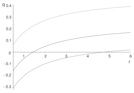
Now we consider the question whether the transition from matter dominance to the coincidence era is compatible with a transition from decelerated to accelerated expansion. This transition implies for and on the late attractor stage. With the help of Eqs. (13), (20) and (22) with the deceleration parameter can be written as
| (46) |
In the present model these acceleration transition constraints
translates into
for the acceleration parameter in the asymptotic regime where
| (47) |
Its derivative
| (48) |
is positive–definite so that the deceleration parameter decreases
monotonically as the Universe expands (see Fig. 1).
Then we find that
| (49) |
and we may write these constraints as , or equivalently
| (50) |
Using Eq. (43) we get
| (51) |
that combined with (49) yields
| (52) |
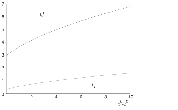
Inserting (52) into (50) and using (45), we find that an accelerating transition implies an upper bound on
| (53) |
and a lower bound on
| (54) |
We note that both bounds grow with the ratio and their values for a perfect fluid (i.e., ) are and respectively (see Fig. 2). The upper bound (53) holds up to the critical ratio where . In the high viscosity regime, above , the upper bound becomes . We also note that the parameter has the lower bound for , that grows with and has a perfect fluid value of . On the other hand , for .
| (55) |
Then, the positive–definite character of the quintessence potential, hence of , implies that the feasible region in parameter space has the upper bound . For CDM it reads and .
The density ratio at the beginning of the accelerated expansion is given as the root of . Using Eq. (46) we find
| (56) |
We see that also grows with the increase of the bulk dissipative pressure, so that ( for CDM) with the constraint ( for CDM).
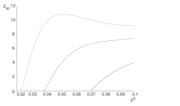
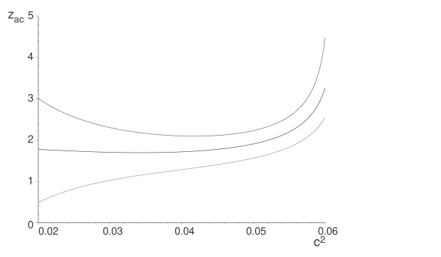
Likewise, the inequalities
must hold. The corresponding redshift is given by
| (57) |
where we have used Eq. (33). We note that the value of the acceleration redshift is model dependent. For CDM models it has been shown to be close to unity TurnerRiess , while it has been argued that coupling between dark energy and dark matter allows for Amendola02 . We have found that this model leads either to or much larger values, depending on the sector of the parameter space (see Figs. 3 and 4).
V Observational constraints
It seems that supernovae of type Ia (SNeIa) may be used as standard candles. Properly corrected, the difference in their apparent magnitudes is related to the cosmological parameters. Confrontation of cosmological models to recent observations of high redshift supernovae () have shown a good fit in regions of the parameter space compatible with an accelerated expansion pedagogical ; Perlmutter98 ; Riess98 ; Efstat ; Perlmutter99 ; Wang99 . We note, however, that models like CDM and QCDM usually require fine tuning to account for the observed ratio between dark energy and clustered matter, while QIM models simultaneously provide a late accelerated expansion and solve the coincidence problem.
Ignoring gravitational lensing effects, the predicted magnitude for an object at redshift in a spatially flat homogeneous and isotropic universe is given by Peebles93
| (58) |
where is its Hubble radius free absolute magnitude and is the luminosity distance in units of the Hubble radius,
| (59) |
For noninteracting QCDM models can be expressed functionally in terms of (assuming that is a constant), so that the history of this index could in principle be reconstructed from the magnitude-redshift data of SNeIa alone. Further, using the conservation equation of the field, the history of the quintessence potential could also be reconstructed. For this reason, many authors have dealt with the recent evolution of .
When quintessence interacts with matter however, the quintessence baryotropic
index looses this preeminent role. To see why it is necessary to plug the
expansion rate in Eq. (59). We first note that Eq. (13)
can be written as .
Then integrating Eq. (20) and inserting in Eq. (22) (for )
we find
| (60) |
where the density ratio in terms of the redshift is given by
| (61) |
So, besides being a functional of the quintessence baryotropic index also becomes a functional of the interaction and dissipative pressures through the effective baryotropic indices. As the histories and cannot be disentangled from in (60), the magnitude-redshift data alone cannot reconstruct even in principle when interactions occur.
| (62) |
This integral can be expressed in terms of the hypergeometric function
| (63) |
where . We have used the sample of high redshift () supernovae of Ref. Perlmutter98 , supplemented with low redshift () supernovae from the Calán/Tololo Supernova Survey Hamuy . This is described as the “primary fit” or fit C in Ref. Perlmutter98 , where, for each supernova, its redshift , the corrected magnitude and its dispersion were computed. We have determined the optimum fit of the QIM model by minimizing a function
| (64) |
where for this data set. This fit yields as the most probable value. We note that means that the Universe is settled at the asymptotic state , with a constant deceleration parameter given by Eq. (49).
In other words, due to the limitations of the magnitude-redshift method (see Ref. Maor and references therein) the currently available set of supernovae located at is unable to provide a clear signature of the turnover from matter dominated decelerated phase to the current accelerated one. Hopefully future observations of type Ia supernovae, such as expected from the proposed SNAP satellite SNAP , combined with other cosmological observations, will provide much severe constraints on the parameters and produce a reliable reconstruction of the evolution of the density ratio. So, for the purpose of fitting to this set of observations, we may use the attractor solution . Then Eq. (63) simplifies to powerlaw ; qsa
| (65) |
where is minus the asymptotic deceleration parameter. So increases with , and corresponds to . On the attractor we have
| (66) |
The optimum fit of this attractor model is given by minimizing the function
| (67) |
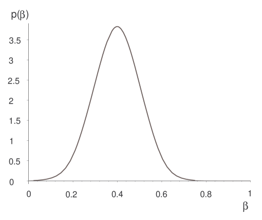
The most likely values of these parameters are found to be , yielding (), and a goodness–of–fit . We estimate the probability density distribution of the parameters by evaluation of the normalized likelihood Lupton93
| (68) |
Then we obtain the probability density distribution for marginalizing over . This probability density distribution is plotted in Fig. 5 and it yields . Hence it can be established that with a confidence level of ; an accelerated superattractor QIM universe is strongly supported by this data set, in agreement with a similar analysis of CDM and QCDM models Perlmutter98 ; Riess98 ; Garnavich98 ; Perlmutter99 .
Stronger bounds on the parameters , and than those obtained in the previous section may be obtained from and estimates of and . The equations to be used are (49), (45) and
| (69) |
obtained by combining Eqs. (43) and (49). For the estimates we take as before , . Besides, Big Bang nucleosynthesis and the fluctuations imprinted on the Cosmic Microwave Background open new windows on the evolution of the quintessence component FJ ; mel ; kneller . Excluding quintessence inflation models (e.g. PV ), primordial nucleosynthesis is probably the earliest epoch from where we can get some information about the density ratio. Hence we approximate the initial density ratio as the ratio at the start up of primordial nucleosynthesis (see the Appendix for further discussion). The quintessence component, evolving under an approximately exponential potential, appears in the early Universe as a form of radiation affecting nucleosynthesis abundance yields and the heights of the acoustic peaks in the cosmic microwave background radiation. When decoupled from matter it behaves like a collisionless, isotropic, and nearly non-clustering component FJ ; dr . Such a non–standard component alters the cooling rate and the upper bound on the change of relativistic energy density is parameterized in terms of the maximum variation in the effective number of neutrino species as , where in the standard model with three massless neutrinos. Then, assuming that the quintessence–matter interaction switches on after nucleosynthesis, we get the bound
| (70) |
Combining it with Eq. (52) and taking into account that dolgov we get for pressureless matter the upper bound on the interaction coefficient
| (71) |
Then, inserting this value in Eq. (49) it follows that
. In other words, a cosmological constant is excluded
in this model. Similarly, from Eq.(69) we get
| (72) |
Besides, assuming a postnucleosynthesis switch on of the interaction, we find
from Eq. (45)
| (73) |
Hence must lie in the range and in the interval . Note that the lower bound (73) is above the critical value , suggesting that viscous effects are important.
VI Concluding remarks
We have presented a spatially homogeneous and isotropic interacting quintessence model that evolves towards a phase of accelerated expansion and simultaneously solves the coincidence problem. It provides a reasonable explanation to the embarrassing question, “why the contributions of dark matter and dark energy (which in principle scale at different rates with expansion) to the overall energy density are of the same order precisely today?” Rather than postulating a potential for the quintessence field and specifying its interaction with the dark matter component, we derived these quantities from the strong coincidence condition (i.e., that the density parameters of these two components tend to constant values at late time). This requirement led us to the stationary condition (Eq.(16)), first obtained in Ref. enlarged , as well as to conclude that the FLRW metric must be spatially flat.
The ratio between the energy densities is seen to evolve from an initial unstable value up to the lower and stable asymptotic value at late time. In terms of these quantities we have introduced the parameter that assess how near (or far away) from the asymptotic state of constant acceleration -see Eq. (32)- our Universe lies. The available data seem to suggest that our Universe is close to the stationary era. On the other hand, they are not sufficient to discriminate our model from the CDM model. Hopefully, the SNAP satellite will provide us with a wealth of high redshift data likely enough to break the degeneracy and infer the redshift at which the Universe began accelerating its expansion.
We note that the quintessence–matter interaction and the dissipative pressure terms imply that the magnitude–redshift relationship is not enough, even in principle, to reconstruct the evolution of these quantities together with the quintessence baryotropic index history. Further independent observational tests are needed for this reconstruction program. Finally, the evolution of cosmological perturbations predicted by this model remains to be studied. This will be considered elsewhere.
Acknowledgements.
D.P. and W.Z. acknowledge partial support by the NATO grant PST:CLG.977973, This work was also partially supported by the University of Buenos Aires under Project X223 and the Spanish Ministry of Science and Technology under grant BFM 2000-C-03-01 and 2000-1322.*
Appendix A
Here we collect some complementary considerations regarding our model. We begin by noting that we consider a universal coupling of the quintessence field to all sorts of matter, either baryonic or not. As our main concern is the investigation of the late universe and a dynamical solution to the coincidence problem, we consider along this stage a simple two-component model: matter (excluding radiation) and quintessence (an additional radiation (relativistic) component would be dynamically irrelevant).
The coupling between matter and quintessence manifests itself as the nonconservation of their partial stress–energy tensors . For the investigation of the dynamics of our homogeneous model, it suffices to specify the projection of this nonconservation equation along the velocity of the whole (comoving) fluid , that for a perfect fluid is
| (74) |
where, for the specific model we have investigated in Sects. III to V, the coupling is with the expansion scalar and , where denotes the total stress energy tensor.
On the other hand, for the investigation of inhomogeneous perturbations of this model, it will be necessary to take into account that the velocity of the components and are different, in general, from the velocity the overall fluid. Also, these fluids may experience acceleration due to pressure gradients or due to their coupling (anomalous acceleration). Perhaps the simplest generalization of (74) to this wider framework is the “longitudinal coupling”
| (75) |
It involves energy transfer between matter and quintessence with no momentum transfer to matter, so that no anomalous acceleration arises. Hence this choice is not affected by observational bounds to a “fifth” force exerted on the baryons. Clearly other generalizations of Eq. (74) could be considered that do involve an anomalous acceleration in matter due its coupling to quintessence. In this regard we note that because of the universal nature of this coupling, it could not be detected by differential acceleration experiments. We also note that the coupling we have proposed is purely phenomenological and the validity of the expression for is restricted to cosmological scales (as it depends on magnitudes that are only well defined in that setting). This means that the form of the coupling at smaller scales remains unspecified, and the requirements for the different couplings that could have a manifestation at these scales are that they give the same (averaged) coupling at cosmological scales and meet the observational bounds from the “local” experiments clifford .
The longitudinal coupling is also a very attractive choice to extend our model to the radiation era, when the dominating matter component is relativistic, as it does not involve deviation of relativistic particles from their geodesics. Indeed the exact solution (28) (valid only for constant ), holds for the matter-quintessence domination era -with in the case of CDM- as well as for the radiation domination era -with . In the usual approximation that drops instantaneously at equality time , all we need to extend our model to the radiation era is to match both solutions of Eq. (13) at (or equivalently at ). Clearly , , the energy densities, and are continuous through this transition, and we can also assume the same for both eras. Hence there is a jump in the slope at given by
| (76) |
where () is the limit from the right (from the left ). That is, falls more steeply in the radiation era than in the matter era. For the combined solution the initial state is the radiation era stationary solution that is larger than the of the matter era solution extrapolated to the radiation era. Then, a lower bound for the matter is also a lower bound for the radiation , and no bound obtained for the parameters is spoiled. In fact better bounds could be obtained using the combined solution.
The extension back in time of the coupling involves another nonuniqueness, and there is no reason to assume that it had the same form also during the early universe. In particular, all couplings containing terms that become negligible in comparison with at late times (e.g. terms like with ) hold the same property of solving the coincidence problem. And the results of our model hold for this class of models in an approximated, asymptotic sense.
In our model we are assuming that the coupling was negligible during the primordial nucleosynthesis. A simple “generalized” coupling with this property is
| (77) |
where the parameter may be chosen at will, so that for and for . So, by choosing as the Hubble parameter at some suitable time after nucleosynthesis (e.g. ), all our results for the late universe stand while the coupling essentially vanishes for times prior to nucleosynthesis end.
Another reason to assume an onset of the interaction at some epoch of the early universe is the high mass of the quintessence field that grows as
| (78) |
for . This means that the mass becomes arbitrary large for early enough times. However, because of the coupling with matter, this very heavy particle could decay into “dangerous” particles like gravitinos, whose decay products would change the baryon–to–photon ratio required by a successful nucleosynthesis (see eg. gravitino ).
References
- (1) S. Perlmutter, Int. J. Mod. Phys. A 15 S1B, 715 (2000).
- (2) S. Perlmutter et al., Astrophys. J. 517, 565 (1999).
- (3) A.G. Riess et al., Astron. J. 116, 1009 (1998).
- (4) P. Brax et al., edits. Proceedings of the XVIIIth IAP Colloquium, “On the nature of dark energy”, held in Paris 1-5 July 2002 (in the press).
- (5) G. Efstathiou, S.L. Bridle, A.N. Lasenby, M.P. Hobson, and R.S. Ellis, Mon. Not. R. Astron. Soc. 303 L47 (1999).
- (6) S. Perlmutter, M.S. Turner and M. White, Phys. Rev. Lett. 83, 670 (1999).
- (7) N.A. Bahcall et al., Science 284, 1481 (1999).
- (8) G. Efstathiou et al., Mon. Not. R. Astron. Soc. 330, L29 (2002).
- (9) A. Melchiorri, talk delivered at the XVIIIth IAP Colloquium, “On the nature of dark energy”, held in Paris 1-5 July 2002, edits. P. Brax et al. (in the press).
- (10) L. Amendola, Phys. Rev D 62, 043511 (2000); D. Tocchini–Valentini and L. Amendola, Phys. Rev. D 65, 063508 (2002).
- (11) W. Zimdahl, D. Pavón and L.P. Chimento, Phys. Lett. B 521, 133 (2001); W. Zimdahl and D. Pavón, to be published in Gen. Relativ. Grav. (2003), preprint astro-ph/0210484
- (12) L.P. Chimento, A.S. Jakubi and D. Pavón, Phys. Rev. D 62, 063508 (2000).
- (13) W. Zimdahl, D.J. Schwarz, A.B. Balakin and D. Pavón, Phys. Rev. D 64, 063501 (2001).
- (14) Chimento L. P., Jakubi A. S. and Zuccalá N.A., Phys. Rev. D 63, 103508 (2001).
- (15) P. de Bernardis et al., Nature 404, 955 (2000); S. Hanany et al., Astrophys. J. 545, L5 (2000); C.B. Netterfield et al., astro-ph/0104460; C. Pryke et al., astro-ph/0104490
- (16) D. Tytler et al., Physica Scripta T85, 12 (2000); J.M. O’Meara et al., Astrophys. J. 552, 718 (2001).
- (17) M.S. Turner, astro-ph/0106035.
- (18) R. Bean, S. H. Hansen, and A. Melchiorri Phys. Rev. D 64 103508 (2001).
- (19) B. Moore, Nature, 370, 629, (1994).
- (20) R. Flores and J. P. Primack, Astrophys. J. 427, L1, (1994).
- (21) A. Burkert and J. Silk, in Dark Matter in Astro and Particle Physics, edited by H.V. Klapdor-Kleingrothaus and L. Baudis (IOP, Bristol, 1999).
- (22) J.F. Navarro, C.S. Frenk and S.D.M. White, Astrophys. J. 462, 563, (1996); ibid 490, 493 (1997).
- (23) B. Moore et al., Monthly Not. R. Astr. Soc. 310, 1147, (1999).
- (24) S. Ghigna et al., astro-ph/9910166.
- (25) D.N. Spergel and P.J. Steinhardt, Phys Rev Lett., 84, 3760, (2000).
- (26) A. Burkert, Astrophys. J. Lett. 534, 143, (2000).
- (27) C. Firmani et al, Monthly Not. R. Astr. Soc. 315, 29, (2000).
- (28) R.N. Mohapatra, S. Nussinov, V. L. Teplitz. e-Print Archive: hep-ph/0111381.
- (29) Rabindra N. Mohapatra and Vigdor L. Teplitz, Phys. Rev. D 62, 063506 (2000).
- (30) W.B. Lin, D.H. Huang, X. Zhang, and R. Brandenberger, Phys. Rev. Lett. 86, 954 (2001).
- (31) D.N. Spergel and P.J. Steinhardt, Phys. Rev. Lett. 84, 3760 (2000); J. P. Ostriker, ibid. 84, 5258 (2000); S. Hannestad, “Galactic halos of self–interacting dark matter,” astro-ph/9912558; C. Firmani et al., Mon. Not. R. Astron. Soc. 315, L29 (2000).
- (32) J. Goodman, New Astronomy 5, 103 (2000).
- (33) M. Kaplinghat, L. Knox, and M.S. Turner, Phys. Rev. Lett. 85, 3335 (2000).
- (34) R. Cen, Astrophys. J. Lett. (to be published), astro-ph/0005206
- (35) S. Colombi, S. Dodelson and L. Widrow, Astrophys. J. 458, 1 (1996).
- (36) R. Schaeffer and J. Silk, ApJ, 332, 1, (1998).
- (37) C.J. Hogan, astro-ph/9912549.
- (38) S. Hannestad and R. Scherrer, Phys. Rev. D 62, 043522, (2000).
- (39) J.J. Dalcanton and C.J. Hogan, astro-ph/0004381.
- (40) C.J. Hogan and J.J. Dalcanton, astro-ph/0002330.
- (41) L.G. Cabral-Rosetti, T. Matos, D. Nuñez, and R.A. Sussman, Class. Quantum Grav. 19 3603 (202).
- (42) D. Pavón, and W. Zimdahl, Physics Letters A 179, 261 (1993).
- (43) M.S. Turner and A.G.Riess, astro-ph/0106051
- (44) L. Amendola, astro-ph/0209494
- (45) L. Wang, R. Caldwell, J.P. Ostriker, and P.J. Steinhardt, Astrophys. J. 530, 17 (2000).
- (46) P.J.E. Peebles, “Principles of Physical Cosmology” (Princeton University Press, Princeton, New Jersey, 1993).
- (47) M. Hamuy, M.M. Phillips, J. Maza, N.B. Suntzeff, R.A. Schommer, and R. Avilés, Astrophys J. 112, 2391 (1996).
- (48) I. Maor, R. Brustein, J. McMahon, and P.J. Steinhardt Phys. Rev. D 65 123003 (2002).
- (49) Levi M., et al., 2000, http://snap.lbl.gov.
- (50) J.A.S. Lima and J.S. Alcaniz, Astron. Astrophys. 348 1 (1999); M. Kaplinghat, G. Steigman, I. Tkachev, and T.P. Walker Phys. Rev. D 59 043514 (1999).
- (51) R. Lupton, “Statistics in Theory and Practice” (Princeton University Press, Princeton, 1993).
- (52) P.M. Garnavich et al., Astrophys. J. 509, 74 (1998).
- (53) P. Ferreira and M. Joyce, Phys. Rev. D 58, 023503 (1998).
- (54) J. P. Kneller and G. Steigman, astro-ph/0210500
- (55) P. J. E. Peebles and A. Vilenkin, Phys. Rev. D 59, 063505 (1999).
- (56) S. Mukohyama, Phys. Lett. B 473, 241 (2000).
- (57) A.D. Dolgov, “Big Bang Nucleosynthesis”,hep-ph/0201107.
- (58) C.M. Will, “The confrontation between general relativity and experiment: A 1998 update”, gr-qc/9811036 ; C.M. Will, Living Rev. Relativity 4, 4 (2001).
- (59) J. Ellis, J. E. Kim and D. V. Nanopoulos, Phys. Lett. B 145, 181 (1984); M. Kawasaki and T. Moroi, Prog. Theor. Phys. 93, 879 (1995); S. Sarkar, Rep. Prog. Phys. 59, 1493 (1996); K. Jedamzik, astro-ph/0112226