Iron K$\alpha$ line profiles and the inner boundary condition of accretion flows

Abstract

Recent X-ray observations have shown evidence for exceptionally broad and skewed iron K$\alpha$ emission lines from several accreting black hole systems. The lines are assumed to be due to fluorescence of the accretion disk illuminated by a surrounding corona and require a steep emissivity profile increasing in to the innermost radius. This appears to question both standard accretion disc theory and the zero torque assumption for the inner boundary condition, both of which predict a much less extreme profile. Instead it argues that a torque may be present due to magnetic coupling with matter in the plunging region or even to the spinning black hole itself. Discussion so far has centered on the torque acting on the disc. However the crucial determinant of the iron line profile is the radial variation of the power radiated in the corona. Here we study the effects of different inner boundary conditions on the coronal emissivity and on the profiles of the observable Fe K$\alpha$ lines. We argue that in the extreme case where a prominent high redshift component of the iron line is detected, requiring a steep emissivity profile in the innermost part and a flatter one outside, energy from the gas plunging into the black hole is being fed directly to the corona.

1 Introduction

The much improved sensitivity of the X-ray satellite XMM Newton is quickly expanding our capability of performing accurate X-ray spectroscopy of accretion powered systems. In several recent observations of accreting black holes, extremely broadened and redshifted iron K$\alpha$ lines have been detected. Wilms et al. (2001) presented the observations of the nearby Seyfert 1 galaxy MCG–6-30-15 in a low-luminosity state and deduced from the iron K$\alpha$ line profile that the reprocessing material must be located in the very innermost part of the accretion flow. Similarly, Miller et al. (2002), found a very broad, skewed Fe K$\alpha$ emission line in the galactic black hole XTE J1650-500 in its very high state. In both cases, not only is the large observed redshift considered as a signature of a rapidly rotating black hole (so that the innermost stable orbit is close to the event horizon and the accretion disc can penetrate much deeper in the potential well), but also the disc emissivity needs to be strongly peaked towards the inner boundary in order to fit the observed line profile. For simplicity, the disc emissivity is usually assumed to have a power-law profile $F(r)\propto r^{-\beta}$ (where $r=R/R_{\rm S}=Rc^{2}/2GM$ is the distance from the center in units of Schwarzschild radii), and the index of such power-law is generally assumed to be given by the accretion disc emissivity index in a standard geometrically thin and optically thick disc [Shakura & Sunyaev 1973]. In this case we expect $\beta<3$. The fact that both Wilms et al. (2001) and Miller et al. (2002) require a larger value of $\beta$ to fit the line profile has prompted speculation that, in the inner disc region, additional energy dissipation must be taking place [Agol & Krolik 2000, Li 2002]. This might be due to magnetic torque exerted by the accreting material in the plunging region at the inner disc boundary [Gammie 1999, Krolik 1999] or to magnetic extraction of the spin energy of the black hole [Li 2002] through magnetic field lines threading the ergosphere and the accretion disc. Such findings have been confirmed by the analysis of a long observation of MCG–6-30-15 with XMM-Newton reported by Fabian et al. (2002). These authors found that “the strong, skewed iron line is clearly detected and is well characterized by a steep emissivity profile within $6GM/c^{2}$ and a flatter profile beyond.”

Here we first make the point that, in the framework of standard, relativistic accretion disc models with zero torque at the inner boundary, the emissivity profile of the hard illuminating X-rays is more centrally peaked than that of the usually assumed standard accretion disc. This is a general property of the energy deposition rate in a magnetic corona above standard accretion discs. Furthermore, the quality of the X-ray spectroscopic data is such that, using our coronal models, we can start considering the nature of the inner boundary condition for relativistic accretion flows. Using a simple analytic formulation, first introduced by Agol & Krolik (2000) to include magnetic stresses at the marginally stable orbit in standard disc equations, we can estimate the effect of a modified inner boundary condition on the observed iron line profiles. In particular, we consider the three following possibilities:

• There is no net torque at the inner boundary (no-torque case; NT);

• Magnetic field lines couple the plunging region to, and exert stress on, the cold, geometrically thin disc only (disc-torque; DT);

• Magnetic field lines couple the plunging region to the vertically extended, magnetically dominated corona only (coronal-thread; CT).

We show that, while in the NT case the coronal emission is more centrally peaked than the disc one (due to the radial dependence of the fraction of energy dissipated there), the effect is greatly enhanced in the CT case, with the strongest deviation from the standard emissivity profile appearing in the innermost coronal region. Although the emissivity profiles again become more centrally peaked when the torque is applied directly to the thin disc (DT), the coronal power is much reduced, and we expect the emission to be completely dominated by the quasi-thermal radiation coming from the optically thick disc.

The structure of the paper is the following: in section 2 we solve the fully general relativistic structure equations for standard geometrically thin and optically thick accretion discs, coupled to a magnetically dominated corona (with the coupling discussed in Merloni, 2003, hereafter M03) and opportunely modified by the inclusion of a term describing the additional dissipation from magnetic stresses at the inner boundary either in the disc or in the corona. In such a way we are able to compute the radial profiles of the hard coronal radiation that illuminates the cold disc and is responsible for the fluorescent iron K$\alpha$ line production (section 3). Then, by means of a simple broken power-law approximation for the coronal emissivity, in section 4, we simulate and compare the expected line profiles for the different cases. In section 5 we discuss a number of possible shortcomings of the model we have adopted, and in section 6 we draw our conclusions.

Figure 1: On the left (panel a), coronal emissivity profiles $F_{\rm c}$ (solid lines) and corresponding standard disc emissivities $Q$ (dashed lines), both normalized to their maximum level, as a function of the disc radius, in units of the inner accretion disc radius (fixed at the marginally stable orbit) for three different values of the dimensionless black hole angular momentum: $a=0$; $a=0.9$ and $a=0.99$, from bottom to top. On the right (panel b), the upper panel shows the location of the innermost stable orbit (dotted line), the radius of maximal coronal emissivity (solid line) and that of maximal disc emissivity (dashed line), all in units of Schwarzschild radii, as functions of the dimensionless black hole spin parameter $a$, for the case of no torque at the inner boundary. In the lower panel the corresponding radial velocity of the gas (in units of the local sound speed) and the relative departure of the gas angular velocity from the Keplerian value (assumed in the computations), at the radius of maximal coronal emissivity are shown.

2 Centrally peaked coronal emissivity: the no-torque case

In Merloni (2003; see also Merloni & Fabian 2002), we have shown how it is possible to build a physically self-consistent analytical model for a thin accretion disc–corona system by solving algebraic equations for the fraction of power released into the corona as a function of the distance from the central (non-rotating) black hole. Here we extend such a treatment to the general relativistic case of accretion discs around rotating black holes by calculating the disc–corona structure equations (presented in the Appendix) which are a generalization of the classical ones first derived by Novikov & Thorne (1973), and take into account both the effects of the presence of a corona on the disc structure and those of the different viscosity prescription on the coronal emissivity profiles.

The nature of viscosity in accretion flows is still one of the most fundamental open questions of black hole astrophysics. At present, magneto-rotational instability [Balbus & Hawley 1991, Balbus & Hawley 1998] is favoured as the primary source of the turbulent viscosity needed to explain the luminosities of accreting black holes. For this reason we expect that the turbulent magnetic stresses responsible for the angular momentum transport in the disc are given by

$$\rho W_{R\phi}\simeq\frac{\langle B_{R}\times B_{\phi}\rangle}{8\pi}\simeq P_{\rm mag}.$$ (1)

Once the relationship between magnetic and disc pressure (given either by the gas or by the radiation) is established, the accretion disc structure can be fully described. This is a long standing issue in accretion disc theory and, in the framework of MRI-driven turbulent viscosity models, can be translated into the uncertainty about the mechanisms by, and the level at, which the disc magnetic field saturates. Numerical simulations are crucial to test and verify different hypothesis on the outcome of the instability and the final scaling of the magnetic pressure. However, full three dimensional MHD simulations of accretion flows that include radiative transfer and is capable to treat radiation-pressure-dominated solutions (on the line of those presented in Turner, Stone & Sano, 2002) are needed, in order to answer the question of the viscosity scaling for luminous thin discs. On the other hand, by means of a more treatable analytic approach, Merloni (2003) has shown that, as the growth rate of the MRI in radiation-pressure-dominated discs is reduced by a factor $c_{\rm g}/v_{\rm A}$ [Blaes & Socrates 2001, Turner, Stone & Sano 2002], where $c_{\rm g}$ is the gas sound speed and $v_{\rm A}$ is the Alfvèn speed, and if the main saturation mechanism for the magnetic field is vertical buoyancy (as would be required in order to produce powerful coronae), then (see also Taam & Lin, 1984; Burm, 1985)

$$P_{\rm mag}=\alpha_{0}\sqrt{P_{\rm gas}P_{\rm tot}},$$ (2)

where $\alpha_{0}$ is a constant (not necessarily smaller than unity, see M03). Then it is easy to show that, locally in the disc, the fraction of power released into the corona [Haardt & Maraschi 1991, Svensson & Zdziarski 1994] is given by

$$f(R)\simeq\sqrt{2\alpha_{0}}\left(1+\frac{P_{\rm rad}(R)}{P_{\rm gas}(R)}\right)^{-1/4}.$$ (3)

The first important implication of the above result is that the coronal fraction $f$ is reduced when radiation pressure dominates. As radiation pressure is more and more dominant with increasing accretion rates, a dependency of the spectral properties of an accreting source (that are very sensitive to the fraction of power released in the hot, optically thin corona) on the accretion rate is introduced. This may be relevant, for example, for understanding spectral transition in galactic black hole binaries [Merloni & Fabian 2002].

Figure 2: The profiles of the coronal fraction $f(R)$ for $\Delta\epsilon=0$ (NT, thick solid lines) and for the case of disc torque (DT) with $\Delta\epsilon=0.05,0.1,0.5$ (dashed lines, $\Delta\epsilon$ increasing from top to bottom). The dimensionless black hole spin $a=0.99,0.9,0.7,0$ is indicated in the different panels. The dimensionless accretion rate, defined as the ratio of the emerging (accretion) bolometric luminosity to the Eddington one has been kept fixed to $\dot{m}\equiv L_{\rm b,acc}/L_{\rm Edd}=\epsilon(a)\dot{M}_{0}c^{2}/L_{\rm Edd}=0.03$, where $\dot{M}_{0}$ is the constant external accretion rate and $\epsilon(a)$ is the standard radiative efficiency computed in terms of binding energy at $R_{\rm in}=R_{\rm ms}$, which is a function of the dimensionless black hole spin $a$.

At any given accretion rate the coronal emissivity profile $F_{\rm c}(R)$, which determines the intensity of the hard X-ray radiation illuminating the disc at every radius, is given by

$$F_{\rm c}(R)=f(R)Q(R)=\frac{3GM\dot{M}_{0}f(R)}{8\pi R^{3}}\frac{{\cal Q}{\cal B}}{{\cal C}^{1/2}}\;{\rm ergs}\;{\rm cm}^{-2}\;{\rm s}^{-1},$$ (4)

where ${\cal Q}$, ${\cal B}$ and ${\cal C}$ are the relativistic correction factors of Novikov and Thorne (1973), approaching unity at large distances (see Appendix). One of the key feature of such a relativistic solution is the ‘no-torque at the inner boundary’ (in the following, NT) condition. Such a condition ensures that the disc radiative flux vanishes at the inner boundary, and this in turn implies that the ratio of radiation to gas pressure decreases as the inner boundary is approached from outside. In fact, the innermost part of a standard geometrically thin and optically thick disc is always gas pressure dominated if the NT condition is satisfied, and the coronal emissivity should therefore be strongly peaked towards the center.

In order to show this, we have calculated the coronal emissivity profiles for a supermassive black hole ($m=10^{8}$) accreting at about three per cent of the Eddington rate (a rate such that at least a portion of the inner disc is dominated by radiation pressure) and with $\alpha_{0}=0.49$, for different values of the black hole spin. We solve the relativistic disc structure equations, modified by the presence of the corona (see Eq. A2-A11), with the disc-corona coupling given by Eq. (3). An example of the results is shown in Fig. 1a. The emissivity profile of the corona $F_{\rm c}$ is much more strongly peaked than the corresponding disc emissivity profile $Q$. This effect does not depends on neglecting the effects of pressure gradients near the inner boundary. Indeed, as it is also clear from Fig. 1a, the peak of the coronal emissivity is not located near the innermost stable orbit, if “near” here means so close that substantial deviation from the values of the physical quantities computed with the Novikov-Thorne equations should be considered. In fact, the coronal emissivity profile peaks close to the radius where the gas pressure is equal to the radiation pressure. Calculations done for high accretion rate discs, including the effects of pressure gradients, show that the ratio of gas to total pressure increases substantially when going towards the center [Abramowicz et al. 1988], from $r/r_{\rm in}=5/3$ to $r/r_{\rm in}=1$ (see e.g. Fig. 6 of Muchotrzeb & Paczynski, 1982, or Fig. 7 of Abramowicz et al. 1988), even for much higher accretion rates than those we are considering. Indeed, we can compute from our numerical solutions the ratio of the radial velocity at the location of the maximal coronal emissivity, $v_{r}(r_{\rm max})\equiv v_{\rm max}$, and compare it with the local sound speed, to have a measure of the distance between $r_{\rm max}$ and the sonic point. Moreover, the error we make by neglecting pressure gradients can be estimated calculating the relative departure of the gas angular velocity from the Keplerian value at $r=r_{\rm max}$, from the momentum equation in the $r$ direction:

$$\frac{\Delta\Omega}{\Omega_{\rm K}}\equiv\frac{(\Omega^{2}-\Omega_{\rm K}^{2})^{1/2}}{\Omega_{\rm K}}=\frac{1}{r\Omega_{\rm K}}\left(\frac{1}{\rho}\frac{dP}{dr}+v_{r}\frac{dv_{r}}{dr}\right)$$ (5)

In Fig. 1b we show the location of the inner disc radius, of the radius of maximal coronal emissivity and of maximal disc emissivity without corona (upper panel) together with the values of $v_{\rm max}/c_{\rm s}$ and $\Delta\Omega/\Omega_{\rm K}$ (lower panel), as a function of the dimensionless black hole angular momentum $a$ for the NT case. At the location of the maximal coronal emissivity, the radial flow is about three orders of magnitude subsonic and the error we make in neglecting pressure gradient and advective terms is a fraction of a percent.

The coronal emissivity profiles shown in Figure 1a represent an upper limit on the central concentration of hard illuminating X-rays that can be achieved without the need of any kind of energy extraction from matter inside the marginally stable orbit. Comparison of the calculated emissivity profiles with those needed to explain the broad relativistic lines observed in the spectra of the Seyfert 1 galaxy MCG–6-30-15 [Wilms et al. 2001, Fabian et al. 2002], reveals that the radial extent of the region with emissivity index $\beta>3$ (the “core” region, see below) is probably too small in the NT scenario to account for the observations. In the next section we investigate the effects of applying a torque at the inner disc boundary on the coronal emissivity profiles.

3 Torque at the inner disc boundary: thin vs. thick discs

The original idea that magnetic field inside the radius of marginal stability ($R_{\rm ms}$) may alter the dynamics of accreting material and act to effectively torque the disc at its inner boundary was already mentioned in the early works on black hole accretion discs (e.g. in Page & Thorne, 1974), although the standard hypothesis, in the following three decades of accretion disc research, has been that of no-torque at the inner boundary (see Abramowicz & Kato, 1989, and references therein). When the NT inner boundary condition is adopted, the maximal energy per unit mass available to be radiated by the accretion disc is uniquely determined by the binding energy at the innermost stable orbit and this fixes the efficiency of accretion. On the other hand, if dynamically important magnetic fields in the plunging region exert significant stresses on the disc (disc torque condition, in the following DT), the available energy per unit mass increases and the efficiency may even reach values greater than unity, if magnetic stress can be exerted on the disc from material that has plunged into the ergosphere, thus effectively tapping the rotational energy of the black hole [Krolik 1999, Gammie 1999, Agol & Krolik 2000]. As a consequence, the nature of the inner disc boundary condition, and in particular the extent of the torque exerted by the plunging gas on the accretion flow, depends on the complicated nature of the (turbulent) angular momentum transport in the disc and in particular on the level of the saturation magnetic field inside the disc [Reynolds & Armitage 2001, Krolik & Hawley 2002]. The recent MHD simulations of Hawley and Krolik (2002), which are the ones with the best resolution to date, seem to confirm the idea that magnetized discs do not satisfy the no-torque at the inner boundary condition, showing that the stress generated by the MHD turbulence does not vanish near the marginally stable orbit.

There is in fact a contrasting argument in such a debate. Indeed, all the simulations that have shown signs of magnetic stress inside the marginally stable orbit were non-radiative, and involved moderately thick discs (very thin, radiatively efficient discs are of course much harder to simulate). Thinner discs being denser, the Alfvèn speed is reduced in their inner part, and maintaining the causal connection between the magnetized gas in the plunging region and the disc should be more difficult. Indeed, Afshordi & Paczynski (2002), by studying a numerical model of a steady state, thin and isothermal accretion disc, argued that the NT inner boundary condition is appropriate, provided that the structure carrying the stress in the disc (likely the magnetic field) has a scaleheight much smaller that the radius, i.e. is itself geometrically thin (see also Li, 2003).

It is worth stressing here that the very existence (and the variability properties) of broad and redshifted fluorescent Iron K$\alpha$ lines in the spectra of accreting black holes, put constraints on the disc models: the discs that produce them have to be cold (not too highly ionized), optically thick to Compton scattering and illuminated by a strongly variable source of hard X-rays. Clearly, non-radiative thick accretion flows, as those simulated by Hawley and Krolik (2002), do not satisfy those conditions.

Therefore, beside the no-torque (NT) and the disc-torque (DT) boundary conditions advocated, respectively, by Paczynski and collaborators and by Krolik and collaborators, we envisage a third plausible alternative, applicable to the case in which a geometrically thin, cold disc is indeed present together with the hotter coronal phase, as inferred from the detection of broad iron K$\alpha$ fluorescent lines. The proposed geometry for the inner flow is the following: a cold thin disc, with no torque at the inner boundary, giving rise to the observed broad lines via reflection of hard X-ray photons, is surrounded by a magnetically dominated [Merloni & Fabian 2001] corona. Magnetic field lines that penetrate the ergosphere at high latitude above the equatorial plane are connected to the coronal plasma, and the torque exerted by the rotation of the inertial frames transports energy into the corona (coronal thread case, CT). This is in practice a generalization of the Blandford-Znajek [Blandford & Znajek 1977] mechanism, where the energy extracted from the rotating hole instead of powering a relativistic outflow is dissipated, via magnetic reconnection, in the corona. The coronal emissivity profile can then be more centrally peaked than in the NT case, because of the excess field dissipation in its innermost part.

Figure 3: The profiles of the coronal fraction $f(R)$ for $\Delta\epsilon=0$ (NT, thick solid lines) and for the case of extra energy dissipation in the corona (CT) with $\Delta\epsilon=0.05,0.1,0.5$ (dashed lines, $\Delta\epsilon$ increasing from bottom to top). The dimensionless black hole spin $a=0.99,0.7$ and the index of coronal dissipation $q_{e}$ are indicated in each different panel. The dimensionless accretion rate, defined as the ratio of the emerging bolometric luminosity to the Eddington one has been kept fixed to $\dot{m}\equiv L_{rmbol}/L_{\rm Edd}=\epsilon(a)\dot{M}_{0}c^{2}/L_{\rm Edd}=0.03$.

In the following sections we treat separately the two extreme case of a torque applied to the thin disc only (DT, section 3.1) and of a direct magnetic connection between the black hole and the coronal plasma (CT, section 3.2). First, we solve the equations for the coupled accretion disc–corona system and derive the coronal emissivity profiles in the two cases, then (section 4) we discuss their effects on the properties of the fluorescent iron lines profiles.

3.1 Torque exerted on the thin disc

We follow here the argument presented by Krolik (1999) and adopt the formalism of Agol & Krolik (2000), in particular, we assume nonzero stress at the marginally stable orbit, so that the flux at the disk surface in the fluid frame is not zero there. The relativistic equations for the disc structure discussed in Agol & Krolik (2000) are modified here by the inclusion of a term that takes into account the fraction of power that goes into the corona and supplemented with the coupling provided by Eq. (3). The corona, in this case, is coupled only to the underlying disc and not to the free-falling gas, nor to the black hole horizon.

Using this boundary condition, we have, for the locally generated radiation flux emerging from the disc:

$$F^{\rm DT}(x)=\frac{3}{8\pi}\frac{GM\dot{M}_{0}(1-f)}{R^{3}}\left(\frac{x_{\rm ms}^{3/2}{\cal C}_{\rm ms}^{1/2}\Delta\epsilon}{{\cal C}(x)x^{1/2}}+R_{\rm R}^{\rm NT}\right).$$ (6)

Here $\Delta\epsilon$ is the additional radiative efficiency relative to the one computed in terms of binding energy at $r_{\rm ms}$ (the usual disc efficiency, $\epsilon(a)$), $x=R/R_{g}=Rc^{2}/GM$ and ${\cal C}(x)$ is one of the auxiliary functions that incorporate relativistic corrections to disk equations (from Novikov and Thorne 1973, see also the Appendix). $R_{\rm F}^{\rm NT}$ is a factor that represent the relativistic correction factors in the NT case [Novikov & Thorne 1973]; it goes to zero at $R_{\rm ms}$. The corresponding angular momentum conservation equation reads

$$-\int T_{r\phi}^{DT}(z)dz=\frac{\dot{M}_{0}\Omega_{\rm K}(x)}{2\pi}\left(\frac{x_{\rm ms}^{3/2}{\cal D}_{\rm ms}^{1/2}\Delta\epsilon}{{\cal C}(x)x^{1/2}}+R_{\rm T}^{\rm NT}\right)$$ (7)

where in the above formula $R_{\rm T}^{\rm NT}$ represent the torque relativistic correction factor (Novikov and Thorne, 1973), analogous to the one included in the flux formula.

With the help of Eqs.(6) and (7), we can again extract the disc structure equations and find the solutions for the coronal fraction as a function of $R$, for different $\Delta\epsilon$. This is shown in Figure 2, for different black hole dimensionless spin parameters and for three different values of $\Delta\epsilon$, between 0.05 ($\la\epsilon(0)\simeq 0.06$) and 0.5 ($\ga\epsilon(1)\simeq 0.42$). We have fixed the dimensionless accretion rate, defined as the ratio of the bolometric luminosity to the Eddington one $\dot{m}\equiv L_{\rm b,acc}/L_{\rm Edd}=\epsilon(a)\dot{M}_{0}c^{2}/L_{\rm Edd}=0.03$.

As expected, when a torque is applied to the geometrically thin, optically thick disc only, the excess dissipation at the inner boundary reduces the ratio $P_{\rm gas}/P_{\rm rad}$ and, consequently, $f$. The more energy is extracted from the plunging region and transferred to the disc, the less coronal emission is produced in the innermost region of the accretion flow.

As it is well known [Agol & Krolik 2000, Li 2002], when extra torque is applied in the innermost region of an accretion disc, the emissivity profile of the disc itself becomes much steeper. Then, if the coronal fraction does not decrease too rapidly with decreasing distance from the hole, the coronal emissivity may be peaked, too. However, the intensity of the non-thermal coronal flux compared with the disc one is much reduced in the DT case, up to the point where coronal emission becomes negligible. In practice, given our prescription for the disc–corona coupling, a torque applied at the inner boundary of the thin disc only, has the effect of quenching the coronal activity in the innermost part of the accretion flow. In section 4 we will show a few quantitative measures of the amount of peakedness of the coronal emissivity profile, and discuss its observable effects on the iron K$\alpha$ line profiles for different black hole spin parameters and $\Delta\epsilon$. Before that, we examine next the effect of extra energy deposition on the corona itself.

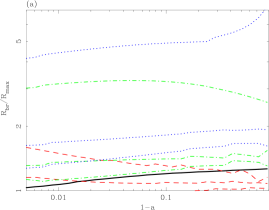
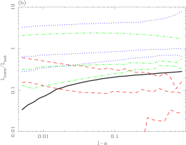
Figure 4: Plots of the ratio $\xi$ of the core radius $R_{\rm br}$ to the radius of maximal coronal emissivity $R_{\rm max}$ (panel a), and of the ratio of the core coronal luminosity $L_{\rm core}$ (computed from $R_{\rm max}$ to $R_{\rm br}$), to the outer one (from $R_{\rm br}$ to $R_{\rm out}=100R_{\rm S}=200GM/c^{2}$; panel b), both as functions of the black hole dimensionless angular momentum parameter $a$. The thick black solid lines represent values computed for $\Delta\epsilon=0$ (NT). Three disc torque cases are shown with (red) dashed lines for $\Delta\epsilon=0.05,0.1$ and $0.5$, from bottom to top, respectively. CT cases correspond to (green) dot-dashed lines ($q_{e}=4$) and (blue) dotted lines ($q_{e}=4.5$), again going from $\Delta\epsilon=0.05,0.1$ to $0.5$ from bottom to top. In all the calculations, we have fixed the dimensionless accretion rate to $\dot{m}=0.03$.

3.2 The black hole–corona connection

The magnetically dominated plasma in the low-density corona (where Alfvèn speed may become relativistic) may indeed be the repository of most of the energy extracted by electromagnetic processes from a spinning black hole [Krolik 1999, Blandford 2001, Semenov et al. 2002]. In this respect, we may consider the inner part of the magnetically dominated corona as the non-stationary analogous of the force-free magnetosphere envisaged by Blandford & Znajek (1977). The extra energy may also come from an increased coronal activity produced by the strongly magnetized plasma in the plunging region [Gammie 1999, Krolik 1999], where efficient reconnection events may disconnect the free-falling plasma from the disc (thus reducing the effective torque at the inner disc boundary), while simultaneously increasing the energy available for coronal heating. The time-averaged effect of such a process of energy extraction and deposition (whose physical modeling, involving the electrodynamics of a reconnecting field in a curved background spacetime, is beyond the aim of this paper) on the radial profile of the hard X-ray radiation illuminating the underlying cold disc is the generation of a central cusp.

In order to consider the effect of a black hole–corona connection, with the consequent increase of coronal emissivity in the simplest possible way, we apply a similar argument to that presented in the previous subsection. The effect of the excess energy dissipation in the coronal region, is parametrized by the same factor $\Delta\epsilon$ representing the extra radiative efficiency of the accreting gas with respect to the standard value $\epsilon(a)$. However, in this case, we leave unchanged the disc equation for the locally generated flux:

$$F(x)=\frac{3}{8\pi}\frac{GM\dot{M}_{0}(1-f^{*}(R))}{R^{3}}R_{\rm R}^{\rm NT},$$ (8)

as well as the angular momentum conservation equation:

$$-\int T_{r\phi}(z)dz=\frac{\dot{M}_{0}\Omega_{\rm K}(x)}{2\pi}R_{\rm T}^{\rm NT},$$ (9)

which are therefore both identical to the no-torque case.

Then, we modify the expression for the local coronal flux by simply adding a term with a power-law profile:

$$F_{\rm c}^{\rm CT}(R)=\frac{3GM\dot{M}_{0}}{8\pi}\left(\frac{f^{*}(R)}{R^{3}}\frac{{\cal Q}{\cal B}}{{\cal C}^{1/2}}+{\cal K}_{e}R^{-q_{\rm e}}\right)\;{\rm ergs}\;{\rm cm}^{-2}\;{\rm s}^{-1}.$$ (10)

The additional term is normalized in such a way that the extra coronal luminosity $L_{e}=2\int^{\infty}_{R_{\rm in}}2\pi RQ_{e}(R)dR$, where we have defined $Q_{e}(r)=(3/8\pi)GM\dot{M}_{0}K_{e}R^{-q_{\rm e}}$, is equal to $\Delta\epsilon\dot{M}_{0}c^{2}$, and thus we have

$${\cal K}_{e}=\frac{4}{3R_{\rm S}}(q_{\rm e}-2)R_{\rm in}^{(q_{\rm e}-2)}.\Delta\epsilon$$ (11)

Here we need to introduce a new definition of the fraction of power released into the corona. We define $f(R)=F^{\rm CT}_{\rm c}(R)/Q(R)=f^{*}(R)+f^{\rm e}(R)$, where now $f^{*}(R)$ is the (usual) fraction of dissipated accretion energy deposited into the corona (bound to be less than unity, see section 2), that enters the disc structure equations, while $f^{\rm e}(R)$ is the additional coronal energy in magnetic field lines connected to the plunging gas at moderate-to-high latitude. As opposed to the DT case, here the more the energy extracted from the black hole (i.e. the bigger $\Delta\epsilon$), the larger the coronal fraction $f(R)$. Indeed, as expected, in the innermost disc region, the coronal fraction, i.e. the ratio of the energy dissipated in the optically thin, hot, magnetically dominated corona to the total gravitational energy locally dissipated by the accretion flow, $Q$, may be larger than unity. This is clearly shown in Figure 3, where, again, we show the profiles of $f(R)$ for both highly and moderately spinning black holes, $a=0.99$ and $a=0.7$, for two different values of the index $q_{\rm e}$ and for three different values of $\Delta\epsilon$, between 0.05 and 0.5. Globally, we can define the integrated fractions of power released into the corona in the following way:

$$<f^{*}>\equiv\frac{2\int^{\infty}_{R_{\rm in}}2\pi Rf^{*}(R)Q(R)dR}{2\int^{\infty}_{R_{\rm in}}2\pi RQ(R)dR}\equiv\frac{L_{\rm c}}{L_{\rm b,acc}}.$$ (12)

Then we get, for the global value of the fraction of power released into the corona, $<f>$:

$$<f>=\frac{L_{e}+L_{\rm c}}{L_{\rm b,acc}}=\frac{\Delta\epsilon}{\epsilon(a)}+<f^{*}>,$$ (13)

from which we deduce that the extra term due to the energy transported from inside $R_{\rm ms}$ and released into the corona, $<f^{\rm e}>$ is given by the ratio $\Delta\epsilon/\epsilon(a)$ of the extra radiative efficiency to the standard (accretion) one.

4 Effects on the Fe K$\alpha$ line profiles

In order to estimate the effect of the coronal emissivity profiles on the shape of the fluorescent Iron K$\alpha$ line produced by the underlying cold, optically thick disc, we have approximated the computed $F_{\rm c}(r)$ with a double power-law (see Fabian et al., 2002, for an application to the observation of MCG–6-30-15), assuming that the inner radius corresponds to the radius of maximal coronal emissivity ($R_{\rm in}=R_{\rm max}$). For the inner core, extending from $R_{\rm max}$ out to a break radius $R_{\rm br}$, we have approximated the peaked profile with an emissivity index $\beta=4$, the same for all the computed profiles. Thus, for the normalized coronal flux we have

$$F_{\rm c}(R) = \left(\frac{R_{\rm max}}{R}\right)^{4}\;\;\;\;{\rm for}\;\;R_{\rm max}<R<R_{\rm br}$$

$$F_{\rm c}(R) = \left(\frac{R_{\rm max}}{R_{\rm br}}\right)^{4}\left(\frac{R_{\rm br}}{R}\right)^{\beta_{2}}\;\;\;\;{\rm for}\;\;R_{\rm br}<R<R_{\rm out}.$$ (14)

By fitting such a profile to the calculated $F_{\rm c}$, we find the core radius $R_{\rm br}$ and the emissivity index, $\beta_{2}$, of the outer, flatter part.

Also, returning radiation [Cunningham 1976] has to be taken into account. This can be done approximately, by using the analytic fitting formula for the fraction of the returning radiation to the locally generated one of Agol & Krolik (2000). For $R_{\rm out}\ga 10R_{\rm in}$ such a fraction, $R_{\rm ret}$ can be approximated with a constant, that we denote $R_{\rm ret,\infty}$. The returning flux then scales as $r^{-3}$:

$$F_{\rm ret}(R)=R_{\rm ret,\infty}Q(R_{\rm out})\left(\frac{R_{\rm out}}{R}\right)^{3}.$$ (15)

We can then introduce the integrated luminosity from the core region $L_{\rm core}=4\pi\int^{R_{\rm br}}_{R_{\rm max}}[F_{\rm c}(R)+F_{\rm ret}(R)]RdR$ (and, correspondingly, that of the outer region $L_{\rm out}=4\pi\int^{R_{\rm out}}_{R_{\rm br}}[F_{\rm c}(R))+F_{\rm ret}(R)]RdR$). By integrating these expressions, we get, for the relative luminosity of the two regions, (for $\beta_{2}\neq 2$)

$$\frac{L_{\rm core}}{L_{\rm out}}=\frac{\beta_{2}-2}{2}\left(\frac{(\xi^{2}-1)+2A\xi^{4}\chi^{3}(\xi-1)}{(1-\chi^{(2-\beta_{2})})+(p-2)A\xi^{4}\chi^{2}(\chi-1)}\right),$$ (16)

where $\xi=R_{\rm br}/R_{\rm max}$, $\chi=R_{\rm out}/R_{\rm br}$ and $A=R_{\rm ret,\infty}Q(R_{\rm out})$.

Both $\xi$ and $L_{\rm core}/L_{\rm out}$ can be used as measures of the peakedness of the coronal emissivity profile. The values of these two quantities determines the profile of the fluorescent iron line produced by the reflection of the illuminating coronal radiation on the cold disc. In Figure 4a we plot the ratio $\xi=R_{\rm br}/R_{\rm max}$ of the break radius to the inner radius as a function of the black hole dimensionless spin $a$, for different values of $\Delta\epsilon$, for the cases of DT, CT and NT. In Figure 4b we plot the ratio $L_{\rm core}/L_{\rm out}$ of the luminosity of the coronal core region to the luminosity of the outer coronal region. These figures show that the inner core in the DT case is less prominent than in the NT case for $a<0.99$ and $\Delta\epsilon<0.1$. Only for $\Delta\epsilon\ga 0.5$ do the coronal emissivity profiles in the DT case become substantially peaked. On the other hand, for the coronal-thread case (CT), already for $\Delta\epsilon=0.05$ is the ratio $L_{\rm core}/L_{\rm out}$ larger than in the NT case. Its value increases rapidly for increasing $\Delta\epsilon$ and $q_{\rm e}$.

To compute the line profiles we have adopted the Laor (1991) model as implemented in XSPEC. Each line is the sum of two components, one produced by the core, the other by the outer region. The model for each component has the following parameters: inner and outer radius, emissivity index $\beta$, line energy, inclination angle and overall normalization. In all cases, the line energy was fixed to 6.4 keV, the emissivity index of the core region to $\beta=4$, the outer radius to $100R_{\rm S}$ and the inclination angle to 30^∘. The variable parameters that determine the line shape are: the inner radius (coincident with $R_{\rm max}$), the break radius, $R_{\rm br}$ (which is simultaneously the outer radius of the core component and the inner radius of the outer component), the emissivity index of the outer component, $\beta_{2}$, and the normalizations of the two components. These have been fixed by imposing $N_{\rm core}+N_{\rm out}=1$ and taking $N_{\rm core}/N_{\rm out}=L_{\rm core}/L_{\rm out}$ as computed with the help of Eq. 16. Table 1 shows the value of the parameters of the double power-law fit to the coronal emissivity profiles that have been used as inputs into the Laor model used to produce the line profiles shown in figures 5, 6 and 7.

Table 1: Physical parameters (inner radius, $r_{\rm max}$; core radius, $r_{\rm br}$, both in units of Schwarzschild radii; outer emissivity index, $\beta_{2}$; and relative normalizations of the core and outer component), obtained from a double power-law fitting of the coronal emissivity profiles for different values of the black hole dimensionless spin parameter $a$, of the extra radiative efficiency $\Delta\epsilon$, and of the inner boundary condition (T). In the fits, the core emissivity index has been fixed to $4$ and the outer radius to $100R_{\rm S}$.

Model parameters				Fit parameters
T	$a$	$\Delta\epsilon$	$q_{\rm e}$	$r_{\rm max}$	$r_{\rm br}$	$\beta_{2}$	$N_{\rm core}$	$N_{\rm out}$
NT	$0.99$	$0$	–	$0.873$	$0.897$	$2.06$	$0.068$	$0.932$
NT	$0.9$	$0$	–	$1.49$	$1.78$	$1.97$	$0.169$	$0.831$
NT	$0.7$	$0$	–	$2.33$	$2.88$	$1.90$	$0.194$	$0.806$
NT	$0.1$	$0$	–	$4.27$	$5.40$	$1.81$	$0.219$	$0.781$
DT	$0.99$	$0.1$	–	$0.734$	$0.826$	$2.11$	$0.112$	$0.888$
DT	$0.9$	$0.1$	–	$1.15$	$1.25$	$2.06$	$0.086$	$0.914$
DT	$0.7$	$0.1$	–	$1.67$	$1.83$	$2.01$	$0.088$	$0.912$
DT	$0.1$	$0.1$	–	$2.79$	$3.02$	$2.02$	$0.077$	$0.923$
DT	$0.99$	$0.5$	–	$0.734$	$1.09$	$2.30$	$0.331$	$0.669$
DT	$0.9$	$0.5$	–	$1.15$	$1.51$	$2.23$	$0.241$	$0.759$
DT	$0.7$	$0.5$	–	$1.67$	$2.11$	$2.25$	$0.210$	$0.790$
DT	$0.1$	$0.5$	–	$2.79$	$3.22$	$2.29$	$0.138$	$0.862$
CT	$0.99$	$0.1$	$4$	$0.734$	$0.999$	$2.57$	$0.267$	$0.733$
CT	$0.9$	$0.1$	$4$	$1.15$	$1.62$	$2.85$	$0.293$	$0.707$
CT	$0.7$	$0.1$	$4$	$1.67$	$2.40$	$3.02$	$0.306$	$0.694$
CT	$0.1$	$0.1$	$4$	$2.79$	$4.30$	$3.11$	$0.361$	$0.639$
CT	$0.99$	$0.5$	$4$	$0.734$	$2.34$	$2.58$	$0.689$	$0.311$
CT	$0.9$	$0.5$	$4$	$1.15$	$3.75$	$2.74$	$0.700$	$0.300$
CT	$0.7$	$0.5$	$4$	$1.67$	$5.06$	$3.06$	$0.679$	$0.321$
CT	$0.1$	$0.5$	$4$	$2.79$	$7.26$	$3.44$	$0.632$	$0.368$
CT	$0.99$	$0.1$	$4.5$	$0.734$	$1.24$	$2.55$	$0.411$	$0.589$
CT	$0.9$	$0.1$	$4.5$	$1.15$	$2.09$	$2.88$	$0.455$	$0.545$
CT	$0.7$	$0.1$	$4.5$	$1.67$	$3.20$	$3.10$	$0.484$	$0.516$
CT	$0.1$	$0.1$	$4.5$	$2.79$	$5.38$	$3.31$	$0.495$	$0.505$
CT	$0.99$	$0.5$	$4.5$	$0.734$	$3.28$	$2.48$	$0.780$	$0.220$
CT	$0.9$	$0.5$	$4.5$	$1.15$	$5.65$	$2.58$	$0.805$	$0.195$
CT	$0.7$	$0.5$	$4.5$	$1.67$	$8.79$	$2.95$	$0.823$	$0.177$
CT	$0.1$	$0.5$	$4.5$	$2.79$	$20.2$	$3.49$	$0.886$	$0.114$

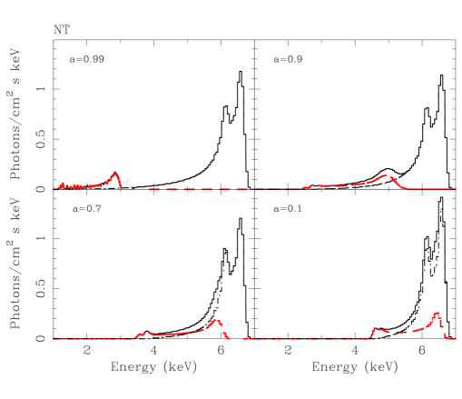
Figure 5: The line profiles calculated from Laor model in the no-torque at the inner boundary case (NT, $\Delta\epsilon=0$), with two components: a core, between the inner radius and the core radius, with steep emissivity profile ($\beta=4$, red dashed lines), and an outer region, from the core radius to the outer radius, with a more shallow emissivity profile. The solid lines represent the total line emission. Four different values of the black hole spin are shown.

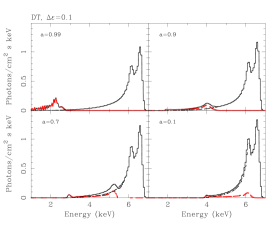
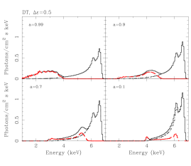
Figure 6: As in Figure 5, in the disc-torque at the inner boundary case (DT), for $\Delta\epsilon=0.1$ (left) and $0.5$ (right) and four values of the spin parameter $a$.

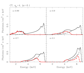
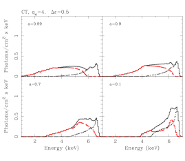
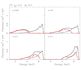
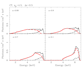
Figure 7: As in Figure 5, in the corona-torque at the inner boundary case (CT), for $\Delta\epsilon=0.1$ (left) and $0.5$ (right), $q_{\rm e}=4$ (top) and $q_{\rm e}=4.5$ (bottom), and four values of the spin parameter $a$.

In Figure 5 we show the composite lines we obtain for the NT case for four values of the black hole spin ($a=0.1,0.7,0.9,0.99$). The red dashed profiles show the line components produced from the core region, while the black, dot-dashed ones those from the outer regions. Obviously, the higher the black hole spin, the more red-shifted is the core-component, which appear as a small excess at low energies. In Figure 6 we show the profiles derived in the CT case for two values of the parameter $\Delta\epsilon$. Comparison with the NT case demonstrate that, for $\Delta\epsilon=0.1$, the redshifted core components are substantially weaker and more redshifted (because $r_{\rm max}$ is smaller in the DT case, see Table 1). For larger $\Delta\epsilon$, the broad red shoulder produced by the core of the coronal emission becomes more evident, especially for rapidly spinning black holes. Finally, in Figure 7 we show the effect of the modified coronal emissivity profile in the case of black hole–corona connection (CT), for two different values of the power-law index of the radial profile of the extra energy dissipation, $q_{\rm e}$. As we expect from the increase of $L_{\rm core}/L_{\rm out}$ with increasing $\Delta\epsilon$ shown in Fig. 4b, the strongly redshifted component of the line, associated with the coronal core is more and more prominent.

The line profiles obtained in the CT with an extra efficiency of the order of 0.1 (and in the DT case for much larger values of $\Delta\epsilon$), are indeed consistent with those observed by XMM Newton in the X-ray spectrum of the Seyfert 1 galaxy MCG–6-30-15 [Fabian et al. 2002], indicating the possibility that dissipation of rotational energy of the black hole tapped by electromagnetic processes has indeed been observed. The calculation we have performed clearly demonstrate that the line profiles are more sensitive to energy of the gas in the plunging region (and/or in the ergosphere) being magnetically transported and dissipated into the corona rather than into the disc, in the sense that the same amount of extra luminosity (additional to the bolometric accretion one) produces much stronger effects in the CT case than in the DT one.

5 Discussion

The calculations we have presented in order to include the effects of different inner boundary conditions into observables are obviously oversimplified, and we discuss below the main uncertainties that may affect our conclusions.

First of all, we only considered stationary solutions of the accretion equations. As clearly demonstrated by a number of simulations [Reynolds & Armitage 2001, Hawley & Krolik 2002] the nature of the accretion flow at the inner boundary is intrinsically time dependent, and the angular momentum transport there, which is mediated by the filaments with the higher relative magnetic field [Reynolds & Armitage 2001], can vary strongly on the dynamical timescale. However the line profiles we aim at modeling are usually derived integrating the observed radiation over many dynamical timescales. In fact, a direct comparison of time-resolved spectra could shed some light on the complex time variability of the inner accretion flow.

Also, we apply a (generalized) $\alpha$ stress model to describe angular momentum transport, which may be questionable if, as we assume, the MRI-driven MHD turbulence saturates due to buoyancy of magnetic flux tubes [Balbus & Papaloizou 1999]. But our approach is essentially phenomenological, and the work presented here aims at understanding the most important pieces of information hidden in marginal effects on observable physical quantities (for example, in the iron line profiles) rather than solve a complex theoretical issue. In this respect, the advantage of the simplifying $\alpha$ prescription is to allow a relatively straightforward interpretation of the observations.

Another reason of uncertainties is the identification of the inner edge of the reflecting cold disc (the “reflection edge”, Krolik & Hawley 2002) with the radius of the marginally stable orbit around the central black hole. As discussed in [Krolik & Hawley 2002], the true reflection edge, i.e. the place where the integrated surface density of the disc has declined enough that the disc becomes effectively transparent, may depend on the accretion rate (and on the fraction of power released into the corona), if magnetic stresses in the inner disc are such that the radial inflow accelerates smoothly inward rather that having a sharp transition at $R_{\rm ms}$. Numerical simulations of cold, thin, radiative discs at different accretion rates are clearly needed in order to better verify these hypothesis.

Finally, contrary to the cases of NT and DT inner boundary conditions, where, for a given small number of assumptions, a full self-consistent analytic model can be solved for the disc–corona system, the coronal-thread hypothesis is admittedly more speculative: we do not have a specific model for how the energy can be extracted from the black hole and deposited there (but see discussion at the beginning of section 3.2), and we do not take into account the problem of angular momentum transfer in the corona (our coronae are effectively non accreting). Once again, given all the theoretical uncertainties, we believe it is more appropriate to adopt the simplest assumption about how the energy extracted from the black hole energizes the corona (see section 3.2) and explore its observational consequences.

Given all the above uncertainties, it is obvious that all three kinds of boundary condition we have adopted are highly idealized. None of them is likely to fully describe the physical condition in the innermost part of a turbulent disc surrounded by a magnetically dominated corona. Nonetheless, their predictions for the intensity of the coronal emission compared with the quasi-thermal disc one, for the coronal emissivity profiles and for the shape of the fluorescent Iron K$\alpha$ lines are qualitatively very different in the three cases and relatively easy to distinguish. That is what makes the use of such idealized models worthwhile. In fact, the current observations provides us with enough information to constrain the models. The shape of the iron line is very sensitive to the coronal emissivity profiles. Both the spin of the black hole (through the amount of gravitational redshift the line photons suffer) and the extra efficiency $\Delta\epsilon$ (through the relative intensity of the red wing of the line, which fixes the emissivity index and size of the core region) can in principle be measured. Simultaneous multi-wavelength observations can set limits on the relative fraction of coronal versus disc emission, therefore helping discriminate between the CT and DT cases. The full picture can then emerge after a careful comparison with existing models of all these pieces of informations.

6 Conclusions

Our work demonstrates that detailed spectral analysis of the most broadened and redshifted iron K$\alpha$ lines from accreting black holes (and of their variability) is a fundamental tool with which to constrain both the geometry of the innermost part of the disc-corona system and the nature of the inner boundary condition of relativistic accretion flows.

The emissivity profile to be considered in analysing the data, to which the line shape is very sensitive, must be that of the illuminating flux, and therefore of coronal radiation, rather than that of the disc. When the generation of a magnetically dominated corona is included self-consistently in the relativistic equations for standard accretion discs, the coronal emissivity profiles are usually strongly peaked in the inner part, as far as a portion of the disc is radiation pressure dominated. The extent of such an inner coronal “core” depends crucially on the inner boundary condition. Here we have explored with our calculation three different (idealized) prescriptions: a classical no-torque at the inner boundary condition; a magnetic connection to the plunging region of the cold, geometrically thin disc only (disc-torque) and a magnetic connection to the plunging region of the vertically extended, magnetically dominated corona only (coronal-thread). We show that, while in the NT case indeed the coronal emission is more centrally peaked than the disc one, this effect is much enhanced in the CT case, with the strongest deviation from the standard emissivity profile appearing in the innermost coronal region for larger black hole spin and larger amount of energy tapped from the plunging region (and/or the black hole itself). On the other hand, when the torque is applied directly to the thin disc (DT case), although the emissivity profiles may become again more centrally peaked (for quite large values of $\Delta\epsilon$), the coronal power is much reduced, and we expect the emission to be completely dominated by the quasi-thermal radiation coming from the optically thick disc.

By approximating the exact coronal emissivity profiles with a broken power-law, we have shown how the detailed line profiles are sensitive to the location of the break radius and to the relative normalization of the inner and outer illuminating regions. These parameters depend strongly on the black hole spin, on the amount of extra energy deposited into the corona, and on the nature of the inner boundary condition itself. The recently observed extremely broad and skewed fluorescent lines in the X-ray spectra of the Seyfert 1 galaxy MCG–6-30-15 [Wilms et al. 2001, Fabian et al. 2002], may therefore be read as an indication that the extraction of energy from spinning black holes is most likely mediated by the magnetic corona rather than by the geometrically thin, optically thick accretion disc.

Appendix A Relativistic disc structure equations with modified viscosity law

Following Novikov & Thorne (1973), we define

$${\cal A} = 1+a^{2}x^{-4}+2a^{2}x^{-6}$$

$${\cal B} = 1+ax^{-3}$$

$${\cal C} = 1-3x^{-2}+2ax^{-3}$$

$${\cal D} = =1-2x^{-2}+a^{2}x^{-4}$$

$${\cal E} = =1+4a^{2}x^{-4}-4a^{2}x^{-6}+3a^{4}x^{-8}$$

$${\cal Q} = \frac{1+ax^{-3}}{x(1-3x^{-2}+2ax^{-3})^{1/2}}[x-x_{0}-1.5a\ln(x/x_{0})$$

$$-\frac{3(x_{1}-a)^{2}}{x_{1}(x_{1}-x_{2})(x_{1}-x_{3})}\ln\frac{(x-x_{1})}{(x_{0}-x_{1})}-\frac{3(x_{2}-a)^{2}}{x_{2}(x_{2}-x_{1})(x_{2}-x_{3})}\ln\frac{(x-x_{2})}{(x_{0}-x_{2})}-\frac{3(x_{3}-a)^{2}}{x_{3}(x_{3}-x_{1})(x_{3}-x_{2})}\ln\frac{(x-x_{3})}{(x_{0}-x_{3})}]$$

where $x=\sqrt{Rc^{2}/GM}$, $x_{0}=\sqrt{R_{\rm ms}c^{2}/GM}$, and $x_{1}=2\cos(1/3\cos^{-1}(a)-\pi/3)$, $x_{2}=2\cos(1/3\cos^{-1}(a)+\pi/3)$, $x_{3}=-2\cos(1/3\cos^{-1}(a))$.

• When magnetic stresses are proportional to the geometric mean of gas and total pressure [Merloni 2003], in the case of radiation pressure dominated discs, we obtain the following expressions for disc scaleheight, pressure, density (both calculated at the disc mid-plane), temperature and ratio of the radiation to gas pressure, respectively:

  $$h \simeq 10.6\dot{m}(1-f){\cal A}^{2}{\cal B}^{-3}{\cal C}^{1/2}{\cal D}^{-1}{\cal E}^{-1}{\cal Q}$$ (18)

  $$P \simeq 3.15\times 10^{18}(\alpha m)^{-8/9}r^{-8/3}\dot{m}_{0}^{8/9}{\cal A}^{-16/9}{\cal B}^{8/9}{\cal C}^{-4/9}{\cal E}^{8/9}{\cal Q}^{8/9}\;{\rm dyne}$$ (19)

  $$\rho \simeq 1.29\times 10^{-4}(\alpha m)^{-8/9}r^{3/9}\dot{m}_{0}^{-10/9}(1-f)^{-2}{\cal A}^{-26/9}{\cal B}^{4}{\cal D}^{5/9}{\cal E}^{13/9}{\cal Q}^{-10/9}\;{\rm g\;cm}^{-3}$$ (20)

  $$T \simeq 1.86\times 10^{8}(\alpha m)^{-2/9}r^{-2/3}\dot{m}_{0}^{2/9}{\cal A}^{-2/9}{\cal D}^{-1/9}{\cal E}^{1/9}{\cal Q}^{2/9}\;{\rm K}$$ (21)

  $$\frac{P_{\rm rad}}{P_{\rm gas}} \simeq 7.97\times 10^{5}(\alpha m)^{2/9}r^{-7/3}\dot{m}_{0}^{16/9}(1-f)^{2}{\cal A}^{20/9}{\cal B}^{-4}{\cal D}^{-8/9}{\cal E}^{-10/9}{\cal Q}^{16/9},$$ (22)

  where the dimensionless parameters are defined as: $r=R/R_{\rm S}$, $\dot{m}_{0}=0.06\dot{M}_{0}c^{2}/L_{\rm Edd}$ and $m=M/M_{\odot}$.

• In the gas pressure dominated part of the disc, instead we have:

  $$h \simeq 2.02\times 10^{-2}\xi^{-3/32}(\alpha m)^{-1/10}r^{21/20}\dot{m}_{0}^{1/5}(1-f)^{1/10}{\cal A}{\cal B}^{-6/5}{\cal C}^{1/2}{\cal D}^{-3/5}{\cal E}^{-1/2}{\cal Q}^{1/5}$$ (23)

  $$P \simeq 1.88\times 10^{18}\xi^{3/32}(\alpha m)^{-9/10}r^{-51/20}\dot{m}_{0}^{4/5}(1-f)^{-1/10}{\cal A}^{-1}{\cal B}^{9/5}{\cal D}^{2/5}{\cal E}^{1/2}{\cal Q}^{-4/5}\;{\rm dyne}$$ (24)

  $$\rho \simeq 20.3\xi^{11/32}(\alpha m)^{-7/10}r^{-33/20}(1-f)^{-3/10}\dot{m}_{0}^{2/5}{\cal A}^{-1}{\cal B}^{3/5}{\cal D}^{-1/5}{\cal E}^{1/2}{\cal Q}^{2/5}\;{\rm g\;cm}^{-3}$$ (25)

  $$T \simeq 5.6\times 10^{8}\xi^{-1/4}(\alpha m)^{-1/5}r^{-9/10}\dot{m}_{0}^{2/5}(1-f)^{1/5}{\cal B}^{-2/5}{\cal D}^{-1/5}{\cal Q}^{2/5}\;{\rm K}$$ (26)

  $$\frac{P_{\rm rad}}{P_{\rm gas}} \simeq 1.31\times 10^{2}\xi^{-35/32}(\alpha m)^{1/10}r^{-21/20}\dot{m}_{0}^{4/5}(1-f)^{9/10}{\cal A}{\cal B}^{-9/5}{\cal D}^{-2/5}{\cal E}^{-1/2}{\cal Q}^{4/5}.$$ (27)

  The value $\xi\simeq 1/3$, the numerical that takes into account the difference in the vertical density profile that should enter in the definition of the disc scaleheight for a gas pressure dominated disc, can be found by imposing continuity of all physical quantities at the boundary between the two regions (see Merloni, 2001).

References

- [Abramowicz et al. 1988] Abramowicz, M. A. Czerny, B., Lasota, J.-P. & Szuszkiewicz, E., 1988, ApJ, 332, 646.
- [Abramowicz & Kato 1989] Abramowicz, M. A. & Kato, S., 1989, ApJ, 336, 304.
- [Afshordi & Paczynski 2002] Afshordi, N., Paczynski, B., 2002, ApJ, submitted, astro-ph/0202409
- [Agol & Krolik 2000] Agol, E. & Krolik, J. H., 2000, ApJ, 528, 161.
- [Balbus & Hawley 1991] Balbus, S. A. & Hawley, J. F., 1991, ApJ, 376, 214.
- [Balbus & Hawley 1998] Balbus, S. A. & Hawley, J. F., 1998, Rev. Mod. Phys. 70, 1.
- [Balbus & Papaloizou 1999] Balbus, S. A. & Papaloizou, J. C. B., 1999, ApJ, 521, 650.
- [Blaes & Socrates 2001] Blaes, O. & Socrates, A., 2001, ApJ, 553, 987.
- [Blandford 2001] Blandford, R. D., 2001, Prog. Theor. Phys. Supp., 143, 182.
- [Blandford & Znajek 1977] Blandford, R. D. & Znajek, R. L., 1977, MNRAS, 179, 433.
- [Cunningham 1976] Cunningham, C. T., 1976, ApJ, 208, 534.
- [Burm 1985] Burm, H., 1985, A&A, 143, 389.
- [Fabian et al. 2002] Fabian, A. C. et al., 2002, MNRAS, 335, L1.
- [Fabian et al. 2000] Fabian, A. C., Iwasawa, K., Reynolds, C. R. & Young, A. J., 2000, PASP, 112, 1145.
- [Galeev, Rosner & Vaiana 1979] Galeev, A. A., Rosner, R. & Vaiana, G. S., 1979, ApJ, 229, 318.
- [Gammie 1999] Gammie, C. F., 1999, ApJL, 522, L57.
- [Haardt & Maraschi 1991] Haardt, F. & Maraschi, L., 1991, ApJL, 380, L51.
- [Hawley & Krolik 2002] Hawley, J. F. & Krolik, J. H., 2002, ApJ, 566, 164
- [Krolik 1999] Krolik, J. H., 1999, ApJL, 515, L73
- [Krolik & Hawley 2002] Krolik, J. H. & Hawley, J. F., 2002, ApJ, 573, 754
- [Laor 1991] Laor, A., 1991, ApJ, 376, 90.
- [Li 2002] Li, X.-L., 2002, ApJ, 567, 463.
- [Li 2003] Li, X.-L., 2003, astro-ph/0212456
- [Martocchia, Matt & Karas 2002] Martocchia, A., Matt, G. & Karas, V., 2002, A&A, 383, L23
- [Merloni 2001] Merloni, A., 2001, PhD thesis.
- [Merloni 2003] Merloni, A., 2003, MNRAS, submitted.
- [Merloni & Fabian 2001] Merloni, A. & Fabian, A. C., 2001, MNRAS, 321, 549.
- [Merloni & Fabian 2002] Merloni, A. & Fabian, A. C., 2002, MNRAS, 332, 165.
- [Miller et al. 2002] Miller, J. M. et al., 2002, ApJL, 570, L69.
- [Muchotrzeb & Paczyński 1982] Muchotrzeb, M. & Paczyński, B., 1982, AcA, 32, 1.
- [Novikov & Thorne 1973] Novikov, I. D. & Thorne, K. S., 1973, in Black Holes, ed. C. De Witt & B. De Witt (New York: Gordon & Breach), 343.
- [Page & Thorne 1974] Page, D. & Thorne, K. S., 1974, ApJ, 191, 499.
- [Reynolds & Armitage 2001] Reynolds, C. S. & Armitage, P. J., 2001, ApJL, 561, L81.
- [Sakimoto & Coroniti 1981] Sakimoto, P. J. & Coroniti, F. V., 1981, ApJ, 247, 19.
- [Sakimoto & Coroniti 1989] Sakimoto, P. J. & Coroniti, F. V., 1989, ApJ, 342, 49.
- [Semenov et al. 2002] Semenov, V. S., Dyadechkin, S. A., Ivanov, I. B., Biernat, H. K., 2002, Physica Scripta, 65, 13.
- [Shakura & Sunyaev 1973] Shakura, N. I. & Sunyaev, R.A., 1973, A&A, 24, 337.
- [Stella & Rosner 1984] Stella, L. & Rosner, R., 1984, ApJ, 277, 312.
- [Svensson & Zdziarski 1994] Svensson, R. & Zdziarski, A. A., 1994, ApJ, 436, 599.
- [Taam & Lin 1984] Taam, R. E. & Lin, D. N. C., 1984, ApJ, 287, 761
- [Turner, Stone & Sano 2002] Turner, N. J., Stone, J. M. & Sano, T., 2002, ApJ, 566, 148.
- [Wilms et al. 2001] Wilms, J., Reynolds, C. S., Begelman, M. C., Reeves, J., Molendi, S., Staubert, R. & Kendziorra, E., 2001, MNRAS, 328, L27.