On the linear filters for point source extraction of the Planck mission

Abstract

The manifestation of point sources in the upcoming Planck maps is a direct reflection of the properties of the pixelized antenna beam shape for each frequency, which is related to the scan strategy, pointing accuracy, noise properties and map-making algorithm. In this paper we firstly compare analytically two filters for the Planck point source extraction, namely, the adaptive top-hat filter (ATHF), the theoretically-optimal filter (TOF). Our analyses are based on the premise that the experiment parameters the TOF assume and require are already known: the CMB and noise power spectrum and a circular Gaussian beam shape and size, whereas the ATHF does not need any a priori knowledge. The analyses show that the TOF is optimal in terms of the gain after the parameter inputs. We simulate the Planck HFI 100 GHz channel with elliptical beam in rotation to test the efficiency of the TOF and the ATHF. We also apply the ATHF on the WMAP Q-band map and the derived map (the foreground-cleaned map by Tegmark, de Oliveira Costa & Hamilton) from the WMAP 1-year data. The uncertainties on the angular power spectrum will hamper the efficiency of the TOF. To tackle the real situations for the Planck point source extraction, most importantly, the elliptical beam shape with slow precession and change of the ellipticity ratio due to possible mirror degradation effect, the ATHF is computationally efficient and well suited for the construction of the Planck Early Release Compact Source Catalogue.

1 Introduction

The observation of cosmic microwave background (CMB) radiation by ESA Planck mission will be able to provide the understanding of our Universe with many key cosmological parameters with unprecedented precision. The signal received from the sky, however, will contain not only the CMB radiation, but also foreground emissions such as synchrotron, dust, free-free emission, Sunyaev-Zel’dovich effect from galaxy clusters and extra-galactic point sources. Removing foreground contaminations is therefore one of the main tasks for the Planck mission. Of these different foreground emissions, the purpose for extraction of extra-galactic point sources has two folds: to separate the foregrounds from the underlying CMB signals to achieve the scientific goal of the Planck mission as this type of foreground contamination is rather non-Gaussian. On the other hand, the whole sky coverage and a wide range of the Planck observing frequencies provide an opportunity for producing the extra-galactic point source catalogue, most notably, the proposed Early Release Compact Source Catalogue (ERCSC), which will be released in roughly 7 months when the full sky is covered once.

Recently, the NASA Wilkinson Microwave Anisotropy Probe (WMAP ) experiment [Bennett et al. 2003a] has demonstrated the importance of the component separation tools for extraction of CMB power spectrum from the raw data. One of the sources with localized peculiarities of the CMB sky is from the point source contamination. For the WMAP mission, the catalogue of the radio point sources was obtained [Bennett et al. 2003b, Pierpaoli 2003] and the final CMB maps were cleaned from the point source contribution.

The WMAP channels at high frequency correspond to the Planck LFI frequency range, in which the contamination of point sources seems 3 times higher than that from the WMAP . For the Planck HFI channels, the point sources are expected to be more significant regarding the issue of component separation and of point source catalogue.

In this paper, we compare the theoretically-optimal filter [Tegmark & de Oliveira-Costa 1998] (hereafter TOF) and the adaptive top-hat filter [Chiang et al. 2002b] (ATHF) proposed for extra-galactic point source detection. Theoretically speaking, the filter proposed by Tegmark & de Oliveira-Costa [Tegmark & de Oliveira-Costa 1998] is optimal in terms of the gain factor. The gain factor is an indicator of the amplitude enhancement of point sources relative to the background. By ‘theoretically’ we mean that the required information input for this filter is known: the CMB and the noise power spectrum, and the circular beam shape and size. This filter is known as a ‘Matched Filter’ in the field of signal processing.

A lot of effort has been devoted to the development of other linear filters [Cayón et al. 2000, Vielva et al. 2001, Sanz, Herranz & Martínez-González 2001, Vio, Tenorio & Wamsteker 2002, Barreiro et al. 2003, Vielva et al. 2003], namely the spherical Mexican Hat Wavelet (MHW), and the so-called pseudo-filter. Vio et al. (2002) and Barreiro et al. (2002) have performed the comparison between the TOF and the pseudo-filter. Vielva et al. (2001, 2003) have applied the MHW on simulation data for the Planck mission.

The Planck in-flight beam shape properties are crucial in connection with the point source extraction. There are many issues regarding the in-flight antenna beam shape properties and its reconstruction [Burigana et al. 2001, Fosalba, Doré & Bouchet 2002, Chiang et al. 2002a, Naselsky et al. 2002]. First of all, according to optics calculations the main beams are not circular Gaussian [Burigana et al. 2001], but elliptical, which is normally formulated as bivariate Gaussian functions. Secondly, with the most likely scan strategy, the inclination angle of the beam is not all parallel through the sky due to possible precession of its spin axis, but is rather slowly rotating along circular scans. Note that this slow rotation of the antenna beam is different from the balloon-borne experiments such as MAXIMA-1, which has a fast rotating beam [Wu et al. 2001], or WMAP, in which the pixels have hits of multiple orientations [Page et al. 2003], and therefore a resultant quasi-symmetric pixel-beam. Furthermore, there could exist mirror degradation effect during the approximately 15-month routine operation of the Planck mission [Naselsky et al. 2002], which will mimic the change of the inclination angle and the shape of the beam. The combined effect from the above-mentioned factors will cause the in-flight beam shape to change with time not only its ellipticity ratio $\sigma_{+}/\sigma_{-}$, where $\sigma_{+}$ and $\sigma_{-}$ are the major and minor axis of the ellipse, but also the inclination angle. There are also some minor effects such as the issues on pointing accuracy and the noise properties that could also mimic the beam degradation. The filters which assume a circular Gaussian beam for point source extraction will need corresponding modifications.

The adaptive top-hat filter is flexible for real situations. The ATHF is similar to the so-called Gabor transform of the signal, using a adaptive width of the kernel. The ATHF has a top-hat shape with two cut-off scales working in harmonic domain. The two cut-off scales $\ell_{\max}$ and $\ell_{\min}$ serve to cut down the unwanted power from both sides of the power spectrum. Simultaneously, the two scales retain the essential part of power spectrum where the convolution (by the beam) of point sources is most pronounced.

We also propose a median filtering technique for removing the point source from the maps. The median filter can be used on combination with any methods of point source detection in order to increase the precision of the CMB map reconstruction.

The layout of this paper is as follows. In Section 2 we discuss the antenna beam shape properties by firstly introducing the Planck scan strategy and the definition of the window function. In Section 3 we present the detailed analysis on the theoretically-optimal filter (TOF) (the Matched Filter) and the adaptive top-hat filter (ATHF). In Section 4 We compare by simulations the TOF and the ATHF on gain capability on more realistic situations and apply the ATHF on Discussions and conclusion are in Section 5.

2 The Planck antenna beam shape properties

2.1 The scan strategy

The manifestation of point sources in the upcoming Planck maps is a direct reflection of the properties of the pixelized antenna beam shape, which is related to the scan strategy, pointing accuracy, map-making algorithm and the extraction of the systematic effects from the time-ordered data (TOD) set and pixelized maps as well. Before our analysis of point source problem, in particular, for the Planck Early Release Compact Source Catalogue (ERCSC), we need to describe the Planck experiment when the TOD contain the information about the signal (and noise) from a large number of circular time-ordered scans [Delabrouille, Patanchon & Audit 2002, Chiang et al. 2002a]. Below we assume for simplicity that the systematic features are already removed and the instrumental noise is Gaussian white noise. In the temporal domain the observed signal $m_{t}$ is the combined signal $d_{t}$ of the CMB and foregrounds from the sky (hereafter beam-convolved ‘sky signals’), plus random instrumental noise $n_{t}$,

$$m_{t}=d_{t}+n_{t}$$ (1)

where

$$d_{t}=\sum_{\ell=0}^{\infty}\sum_{m=-\ell}^{\ell}B_{t,\ell m}a_{\ell m}Y_{\ell m}({\mbox{\boldmath$r$}}_{t}),$$ (2)

and $B_{t,\ell m}$ is the multipole expansion of the time-stream beam $B_{t}({\mbox{\boldmath$r$}}_{t})$. In Eq. (2) $a_{\ell m}$ are the corresponding multipole coefficients of the CMB and foreground signal expansion on the sphere and $Y_{\ell m}$ are the spherical harmonics.

Following Tegmark & Efstathiou [Tegmark & Efstathiou 1996] we also assume that map making algorithm is linear. Thus the signal in each pixel $s_{p}$ should have the following relation

$$d_{t}=\sum\limits_{p=0}^{N}{\sf M}_{t,p}s_{p},$$ (3)

where ${\sf M}_{t,p}$ is the corresponding pointing matrix and $s_{p}$ is the sky signals convolved by the pixel beam $B_{p,\ell m}$,

$$s_{p}=\sum_{\ell=0}^{\infty}\sum_{m=-\ell}^{\ell}B_{p,\ell m}a_{\ell m}Y_{\ell m}({\mbox{\boldmath$x$}}_{p}),$$ (4)

${\mbox{\boldmath$x$}}_{p}$ is the two-dimensional vector with its components $x_{p}$ and $y_{p}$ denoting the location on the surface of the sphere. The definition of the pointing matrix ${\sf M}_{t,p}$ depends on the scan strategy of an experiment. Below, as a basic model, we will use the model of the scan strategy of the Planck mission which was discussed by Burigana et al. [Burigana et al. 1998]. Let $s$ be the unit vector along the satellite spin-axis in the anti-Sun direction and $o$ is that along the direction of the optical axis of the telescope. The angle between spin-axis and optical axis is $\alpha_{0}=\cos^{-1}({\mbox{\boldmath$s$}}\cdot{\mbox{\boldmath$o$}})\simeq 85^{\circ}$. The satellite itself will scan the same circle 60 times around the spin-axis at $\Omega=1$ r.p.m.. Each hour the spin-axis is manoeuvred along the ecliptic plane by $\sim 2\aas@@fstack{\prime}5$. Note that for our geometrical model, during the circling of the optical axis around the spin-axis in each step, the inclination of the beam relative to the optical axis are stable. For modelling of the Planck antenna beam shape we will describe the simplest scan strategy with the spin axis right on the ecliptic plane without any additional (regular) modulation (e.g. it can be above or below the plane due to precession). This model reflects the geometrical properties of the beam asymmetry and their manifestation in the pixelized maps. Under the assumptions mentioned above we can now describe the elliptical beam shape model as follows,

$$B_{t}({\mbox{\boldmath$x$}}-{\mbox{\boldmath$x$}}_{t})=\exp\left[-\frac{1}{2}({\sf RU})^{\rm T}{\sf D}^{-1}({\sf RU})\right],$$ (5)

where

$${\sf U}=\left(\begin{array}[]{c}x-x_{t}\\ y-y_{t}\par\end{array}\right),$$ (6)

${\sf R}$ is the rotation matrix which describes the inclination of the elliptical beam,

$${\sf R}=\left(\begin{array}[]{rr}\cos\alpha&\sin\alpha\\ -\sin\alpha&\cos\alpha\end{array}\right),$$ (7)

with $\alpha$ being the inclination angle between $x$ axis and the major axis of the ellipse. The ${\sf D}$ matrix denotes the beam dispersion along the ellipse principal axes, which can be expressed as

$${\sf D}=\left(\begin{array}[]{cc}\sigma^{2}_{+}&0\\ 0&\sigma^{2}_{-}\par\end{array}\right).$$ (8)

The center of the Cartesian coordinate system is denoted by $x_{t}$ and $y_{t}$ at some moment $t$ with $z$ axis along the $o$, and $x$ and $y$ axis on the plane tangent to the celestial sphere. We will choose below the standard orientation of the local Cartesian coordinate system with $x$ axis parallel to the scanning direction.

After some time $\Delta t=2\pi N_{\rm rot}/\Omega$, where $N_{\rm rot}=60$ is the number of the sub-scans, the spin axis of the satellite shall be stepped along the ecliptic plane to ${\mbox{\boldmath$s$}}^{{}^{\prime}}$ with the small deviation $\Delta{\mbox{\boldmath$s$}}={\mbox{\boldmath$s$}}^{{}^{\prime}}-{\mbox{\boldmath$s$}}\sim 2\aas@@fstack{\prime}5$. For a small part of the sky we can neglect the rotation of the Cartesian coordinate system and choose the $x^{{}^{\prime}}$ and $y^{{}^{\prime}}$ axes parallel to $x$, $y$ axis.

The received signals in each pixel $p$ depend on the orientation of the pixel beam $B_{p}({\mbox{\boldmath$x$}})$ and the location of its center [Wu et al. 2001]. For the upcoming Planck non-symmetric spatially-dependent beam, the convolution of the signal with asymmetric beam immediately produces non-Gaussian signature coupled with the underlying signal, which affects the estimation of angular power spectrum. Although the real beam profile (including the sidelobes) are complicated, we begin our analysis from the model of the time-dependent, elliptical beam shape which is applicable up to $\sim\,-30$ dB level. At low amplitude part of the beam shape ($<-30$ dB) the complexity of the beam estimation increase dramatically. Moreover, due to possible precession of the spin axis $s$ (around the standard orientation), which can be described as some additional noise, it is possible to find some transformation of the width of the beam taking into account the statistical properties of the precession. In such a case the angle between the spin axis and the optical axis should be $\phi(t)=\phi_{0}+\nu(t)$, where $\phi_{0}\sim 85^{\circ}=\rm const.$ and $\nu(t)\ll\phi_{0}$ denote a random precession.

2.2 The window function

Due to the scan strategy and (possible) precession, the pixel beam pattern, in principle, should be different for different pixels on the sphere, which means that we need some modification of the standard tools for the $C_{\ell}$ power spectrum extraction by taking into account any possible peculiarities from the bivariate Gaussian beam shape. The finite resolution of the pixel beam means that the signal we receive from the sky is smoothed by the beam,

$$T({\mbox{\boldmath$p$}})=\int d\Omega_{\mbox{\boldmath$n$}}B({\mbox{\boldmath$p$}},{\mbox{\boldmath$n$}})T_{\rm CMB}({\mbox{\boldmath$n$}})$$ (9)

Usually the influence of the pixel beam on the observed signals can be described in terms of the window function [White & Srednicki 1995, Souradeep & Ratra 2001]

$$W_{\ell,({\mbox{\boldmath$p$}},{\mbox{\boldmath$q$}})}^{2}=\frac{4\pi}{2\ell+1}\sum_{m=-\ell}^{\ell}B_{\ell m,{\mbox{\boldmath$p$}}}B^{*}_{\ell m,{\mbox{\boldmath$q$}}}$$ (10)

where $p$ and $q$ denote the positions of the corresponding pixels in the map and

$$B_{\ell m,{\mbox{\boldmath$p$}}}=\int d\Omega_{\mbox{\boldmath$n$}}B({\mbox{\boldmath$p$}},{\mbox{\boldmath$n$}})Y_{\ell m}^{*}({\mbox{\boldmath$n$}})$$ (11)

is the spherical harmonic transform of the beam function pointing in the direction $p$. This window function determines the CMB signal correlation matrix as

$$C_{({\mbox{\boldmath$p$}},{\mbox{\boldmath$q$}})}=\sum_{\ell=0}^{\infty}{2\ell+1\over 4\pi}C_{\ell}W_{\ell,({\mbox{\boldmath$p$}},{\mbox{\boldmath$q$}})}^{2}$$ (12)

In the framework of the Planck mission it is possible to use the flat sky approximation (as a part of the whole sky $C_{\ell}$ harmonic analysis) in order to estimate the point source contamination and beam influence on the high multipole part of the $C_{\ell}$ power spectrum. For such flat sky limit the computation cost is minimal, as we can implement Fast Fourier Transforms (FFT) for the CMB anisotropy. When the sky signal is convolved with an elliptical beam with an angle between its major axis and the scan direction, the temperature becomes

$$T({\mbox{\boldmath$p$}})=\int_{0}^{\infty}\frac{d{\mbox{\boldmath$k$}}}{(2\pi)^{2}}e^{i{\mbox{\boldmath$k$}}\cdot{\mbox{\boldmath$p$}}}B({\sf R}_{\alpha}[{\mbox{\boldmath$k$}}])T_{\rm CMB}({\mbox{\boldmath$k$}}),$$ (13)

where $B$ is the Fourier transform of the beam profile at the origin, and ${\sf R}_{\alpha}[{\mbox{\boldmath$k$}}]$ is the rotation operator with an angle $\alpha$ with respect to the scan direction [Souradeep & Ratra 2001], which can be written explicitly as

$$B({\sf R}_{\alpha}[{\mbox{\boldmath$k$}}])=\exp\left[-\frac{1}{2}({\sf RK})^{\rm T}{\sf D}({\sf RK})\right],$$ (14)

where ${\sf R}$ and ${\sf D}$ are defined as in Eq. (7) and (8) and

$${\sf K}=\left(\begin{array}[]{c}k_{x}\\ k_{y}\end{array}\right).$$ (15)

The window function now can be expressed as [Souradeep & Ratra 2001]

$$W^{2}_{\mbox{\boldmath$k$}}(\alpha,\Delta\theta)=$$ (16)

$$\int_{0}^{2\pi}\frac{d\phi_{k}}{2\pi}e^{i{\mbox{\boldmath$k$}}\cdot\Delta{\mbox{\boldmath$\theta$}}}B({\sf R}_{\alpha}[{\mbox{\boldmath$k$}}])B^{*}({\sf R}_{\alpha+\Delta\theta}[{\mbox{\boldmath$k$}}]),$$

where $\phi_{k}$ is the angle of wave vector ${\mbox{\boldmath$k$}}\equiv(k_{x},k_{y})$ in the $k$ space such that $k_{x}=k\cos\phi_{k}$ and $k_{y}=k\sin\phi_{k}$. Moreover, for the flat sky approximation (and without the influence of the instrumental noise and any peculiarities of the scanning such as precession) we can use the assumption of stable beam orientation, $\alpha=\rm const.$, with the corresponding Fourier image for the elliptical part of the beam shape,

$$B({\mbox{\boldmath$k$}}) = \exp\left[-\frac{\sigma^{2}_{+}(k_{x}\cos\alpha+k_{y}\sin\alpha)^{2}}{2}\right.$$ (17)

$$- \left.\frac{\sigma^{2}_{-}(-k_{x}\sin\alpha+k_{y}\cos\alpha)^{2}}{2}\right]$$

$$= \exp\left[-\frac{k^{2}_{x}}{2a^{2}}-\frac{(k_{y}-k_{x}\frac{b^{2}}{a^{2}})^{2}a^{2}\sigma^{4}}{2}\right]$$

where $\sigma^{2}=\sigma_{+}\sigma_{-}$, $r=\sigma_{+}/\sigma_{-}$, $a^{2}=(\cos^{2}\alpha+r^{2}\sin^{2}\alpha)/r\sigma^{2}$ and $b^{2}=-(r^{2}-1)\sin 2\alpha/2r\sigma^{2}$. Without loss of generality, we can rotate the coordinate system such that $\alpha=0$, and, for small $\Delta\theta$, $\Delta{\mbox{\boldmath$\theta$}}\equiv{\mbox{\boldmath$\theta$}}=(\theta_{x},\theta_{y})$ with $\beta=\arctan(\theta_{y}/\theta_{x})$. The window function can be written as

$$W_{\mbox{\boldmath$k$}}^{2}(\Delta\theta)\equiv W_{k}^{2}(\theta,\beta)=\int_{0}^{\pi}\frac{d\phi_{k}}{\pi}\cos[k\theta\cos(\phi_{k}-\beta)]$$

$$\times \exp\left\{-k^{2}\sigma^{2}r\left[1+(r^{-2}-1)\sin^{2}\phi_{k}\right]\right\},$$ (18)

with the bivariate beam profile

$$B({\mbox{\boldmath$k$}})=\exp\left\{-\frac{k^{2}\sigma^{2}r}{2}\left[1+(r^{-2}-1)\sin^{2}\phi_{k}\right]\right\}.$$ (19)

The integral in Eq. (18) can be expressed analytically [Souradeep & Ratra 2001]. If the asymmetry of the beam shape is low then we can express $W_{k}(\theta)$ as an infinite series in powers of asymmetry parameter $\epsilon_{k}=k^{2}\sigma^{2}(r^{-2}-1)$,

$$W_{k}^{2}(\theta,\beta)=\sum\limits_{n=0}^{\infty}(-1)^{n}(\epsilon_{k})^{n}w_{k,n}$$ (20)

where

$$w_{k,n}=B\left(\frac{1}{2},n+\frac{1}{2}\right)(\cos\beta)^{2n}\exp(-k^{2}\sigma^{2}r)$$

$$\times\sum\limits_{m=0}^{n}\frac{(\tan\beta)^{2m}F_{2}\left(\frac{1}{2}+m,\frac{1}{2},1+n;-k^{2}\theta^{2}/4\right)}{\Gamma(n-m+1)\Gamma(m+1)},$$ (21)

$\Gamma(a)$ and $B(a,b)$ are the Euler Gamma function of the first and the second kind, respectively, and $F_{2}$ is a generalized hyper-geometric function. For beams with symmetric shape where $r=1$ and $\sigma_{+}=\sigma_{-}=\sigma$, we obtain from Eq. (21)

$$W_{k}^{2}(\theta)=J_{0}(k\theta)e^{-k^{2}\sigma^{2}},$$ (22)

where the zeroth-order Bessel function $J_{0}(k\theta)$ corresponds to the standard asymptotic of the Legendre polynomials $P_{\ell}(\cos\theta)\approx J_{0}(k\theta)$ at $k=\ell+1/2$. In a general case when $r\geq 1$ the window function $W_{k}^{2}(\theta)$ is a function of the separation angle $\theta$ and phase $\beta$ as from Eq. (21). This fact reflects the influence of the anisotropy of the beam on the CMB signal after convolution which transforms isotropic CMB signal to anisotropic one.

For applications of the above-mentioned properties of the beam shape and the window function for point source extraction, let us define the mean beam profile as follows,

$$\overline{B}_{\ell}=\frac{1}{2\ell+1}\sum_{m=-\ell}^{\ell}B_{\ell m}.$$ (23)

In the flat sky approximation, taking Eq. (19) into account, the mean beam profile is related to the ellipticity parameter $r$ as

$$\overline{B}(k)=\exp\left[-\frac{k^{2}\sigma^{2}(r^{2}+1)}{4r}\right]I_{0}\left[\frac{k^{2}\sigma^{2}(r^{2}-1)}{4r}\right],$$ (24)

where $I_{0}(x)$ is the Bessel function of the first kind. For the window function $W^{2}(k)$ in the flat sky approximation we have

$$W^{2}(k)=\int_{0}^{\pi}\frac{d\phi}{\pi}\exp\left\{-\frac{k^{2}\sigma^{2}}{r}\left[1+(r^{2}-1)\sin^{2}\phi\right]\right\}$$

$$=\exp\left[-\frac{k^{2}\sigma^{2}(r^{2}+1)}{2r}\right]I_{0}\left[\frac{k^{2}\sigma^{2}(r^{2}-1)}{2r}\right].$$ (25)

The last two approximations play a crucial role in point source extraction. First of all, the actual value of the beam profile at the location of the point source is related to the orientation of the beam as

$$B({\mbox{\boldmath$k$}}) = \overline{B}(k)I_{0}^{-1}\left[\frac{k^{2}\sigma^{2}(r^{2}-1)}{4r}\right]$$ (26)

$$\times \exp\left[-\frac{k^{2}\sigma^{2}(r^{2}-1)}{4r}\cos 2\phi_{{\mbox{\boldmath$k$}}}\right],$$

and is different from the mean beam profile. These differences depend on the position of the point source in the map and for a given value of the flux $S_{i}$ the result of the point source subtraction should be different for different points of location.

3 Optimization of the linear filters

In this section we would like to elaborate for point source extraction the subtleties of the 3 linear filters: the theoretically-optimal filter, the adaptive top-hat filter and the pseudo-filter. The analyses and comparisons are based on the assumption that the beam shapes for all frequency channels are circular Gaussian and are known if required (by the TOF and the pseudo-filter) and the signal properties, both the CMB and pixel noise power spectrum, are known if required (by the TOF). The analysis and comparison is in terms of the gain factor. The gain factor is defined as $R_{\rm f}/R_{\rm i}$, where $R_{\rm f}$ is the signal ${\rm S}_{\rm f}$ to noise ${\rm N}_{\rm f}$ ratio with “${\rm f}$” indicating after convolution by the filter.

3.1 The theoretically-optimal filter

In the following analyses for the theoretically-optimal filter (TOF) we adopt the convention of notation by Tegmark & Efstathiou [Tegmark & Efstathiou 1996], Tegmark & de Oliveira-Costa [Tegmark & de Oliveira-Costa 1998] (hereafter TD98), i.e., the de-convolved power spectrum of the combined signal is defined as

$$C_{\ell}=C_{\ell}^{\rm sky}+\frac{C^{\rm pix}}{W_{\ell}^{2}},$$ (27)

where $C_{\ell}^{\rm sky}$ is the sky signals including CMB and all foregrounds but the point source contribution, $C^{\rm pix}$ is the noise power spectrum, which is taken as $({\rm FWHM}\sigma_{\rm pix})^{2}$, and $W_{\ell}^{2}$ is the window function. Thus the combined (except point sources) power spectrum in the map is $C_{\ell}^{\rm tot-ps}\equiv C_{\ell}W_{\ell}^{2}$. Note that the in-flight beam $B_{\ell m}$ and the window function $W_{\ell}^{2}$ definitely have some error bars caused by possible mirror degradation effects, the galactic foreground contaminations and the instrumental noise. Thus simple inversion of $W_{\ell}^{-2}$ for the power spectrum requires specific renormalization due to the antenna beam shape properties.

The idea to construct the theoretically-optimal filter (TOF) for point source extraction is outlined in TD98. We can write down the signal as the sum of the point source contribution and the rest (TD98)

$$x({\mbox{\boldmath$r$}})=g\sum_{i}S_{i}\delta_{D}({\mbox{\boldmath$r$}}_{i},{\mbox{\boldmath$r$}})+\sum_{\ell m}a_{\ell m}Y_{\ell m}({\mbox{\boldmath$r$}}),$$ (28)

where $\delta_{D}$ is a Dirac delta function, $S_{i}$ is the flux of the point source at the direction ${\mbox{\boldmath$r$}}_{i}$, $a_{\ell m}$ is the coefficients of the signal decomposition with $\langle|a_{\ell m}|^{2}\rangle\equiv C_{\ell}$ as in Eq. (27), $Y_{\ell m}({\mbox{\boldmath$r$}})$ the spherical harmonics, and

$$g=\frac{1}{2k}\left(\frac{hc}{kT_{\rm CMB}}\right)^{2}\frac{[2\sinh(h\nu/2kT_{\rm CMB})]^{2}}{(h\nu/kT_{\rm CMB})^{4}}.$$ (29)

This filter is named as ‘theoretically-optimal’ because it is constructed in such a way that the gain factor will be maximal, i.e., when the ‘observed’ signal, $B\otimes x({\mbox{\boldmath$r$}})$ is convolved with the filter $F$,

$$y({\mbox{\boldmath$r$}}) = g\sum_{i}S_{i}(F\otimes B)({\mbox{\boldmath$r$}}_{i}\cdot{\mbox{\boldmath$r$}})$$ (30)

$$+ \sum_{\ell m}F_{\ell m}B_{\ell m}a_{\ell m}Y_{\ell m}({\mbox{\boldmath$r$}}),$$

the maximization of the ‘signal’ to ‘noise’ ratio (${\rm S}_{\rm f}/{\rm N}_{\rm f}$) will give us the filter shape, where ${\rm S}_{\rm f}$ is the square root of the variance of the point source amplitudes and ${\rm N}_{\rm f}$ now is the rms of the combined signal, both convolved by the filter $F$. Equivalently, we want to maximize

$$R = \frac{g^{2}\langle\sum_{i}\sum_{j}S_{i}S_{j}[(F\otimes B)({\mbox{\boldmath$r$}}_{i}\cdot{\mbox{\boldmath$r$}})][(F\otimes B)({\mbox{\boldmath$r$}}_{j}\cdot{\mbox{\boldmath$r$}})]\rangle}{\sum_{\ell}{(2\ell+1)/(4\pi)}F_{\ell}^{2}W_{\ell}^{2}C_{\ell}}$$ (31)

$$= g^{2}\sum_{i}S_{i}^{2}\frac{\left[\sum_{\ell}{(2\ell+1)/(4\pi)}F_{\ell}\overline{B_{\ell}}\right]^{2}}{\sum_{\ell}{(2\ell+1)/(4\pi)}F_{\ell}^{2}W_{\ell}^{2}C_{\ell}},$$

where $\otimes$ denotes convolution, $B_{\ell m}$ are the coefficients of the spherical harmonic decomposition of the beam profile, $F_{\ell m}$ is the multipole expansion of $F$, and $\overline{B_{\ell}}$ is the mean beam. We thus can obtain the TOF for each Planck frequency channel.

Note that in reaching Eq. (31) the filter is assumed isotropic in the Fourier rings and statistically homogeneous. Thus in the spherical harmonic decomposition this filter has only $\ell$-dependence, but not on the azimuthal numbers $m$. This condition is only valid when the sky signal and the pixel noise are Gaussian. If the sky signal (or the pixel noise) is non-Gaussian, however, then Eq. (31) needs the corresponding modification. For the following analyses we assume for simplicity that the Gaussian assumption is appropriate for the CMB plus foreground.

The determination of the TOF is similar to the definition of functional derivatives definition. Suppose that $\overline{F_{\ell}}$ corresponds to the maximization of the ratio $R$ from Eq. (31), then a small variation $f_{\ell}$ of the shape from the $\overline{F_{\ell}}$ shall shift the function $R(\overline{F_{\ell}}+f_{\ell})$ away from the maximal value $R_{\max}$, which is proportional to the $f_{\ell}$, $f_{\ell}^{2}$…, if $||f||\ll 1$. So we have

$$F_{\ell}=\overline{F_{\ell}}+f_{\ell},$$ (32)

and obtain the following formulae from Eq. (31),

$$\Delta\equiv R(F_{\ell})-R(\overline{F_{\ell}})=g^{2}\sum_{i}S_{i}^{2}\frac{M+Q}{\alpha P},$$ (33)

where

$$M=2\beta\sum_{n}\frac{2n+1}{4\pi}\left[\alpha\overline{B}_{n}-\beta W^{2}_{n}C_{n}\overline{F}_{n}\right]f_{n},$$ (34)

$$\alpha=\sum_{\ell}{2\ell+1\over 4\pi}W_{\ell}^{2}\overline{F_{\ell}}^{2}C_{\ell},$$ (35)

$$\beta=\sum_{\ell}{2\ell+1\over 4\pi}\overline{B_{\ell}}\,\overline{F_{\ell}},$$ (36)

$$Q = \alpha\left(\sum_{n}\frac{2n+1}{4\pi}\overline{B}_{n}f_{n}\right)^{2}$$ (37)

$$- \beta^{2}\sum_{n}\frac{2n+1}{4\pi}W^{2}_{n}f^{2}_{n}C_{n},$$

and

$$P=\sum_{\ell}{2\ell+1\over 4\pi}W_{\ell}^{2}(\overline{F_{\ell}}+f_{\ell})^{2}C_{\ell}.$$ (38)

Equivalently, to maximize the gain factor $R(F_{\ell})$ is to take $M=0$, the condition that the first functional derivative is zero, $\delta R/\delta F_{\ell}=0$. If we assume that the TOF profile is an analytic function, then from Eq. (34) we get

$$\overline{F}_{n}=\frac{\alpha\overline{B}_{n}}{\beta W^{2}_{n}C_{n}}.$$ (39)

As one can see from Eq. (35) and (36) the coefficients $\alpha$ and $\beta$ are also the functionals of the TOF profile. Substituting Eq. (39) into Eq. (35) and (36) we obtain the following relationship between $\alpha$ and $\beta$ functionals,

$$\beta^{2}=\alpha\sum_{\ell}{2\ell+1\over 4\pi}\frac{\overline{B_{\ell}}^{2}}{W_{\ell}^{2}C_{\ell}}$$ (40)

Taking into account the definitions of the $\alpha$ and $\beta$ functionals and Eq. (40), we reach the conclusion that the TOF $\overline{F}_{n}$ from Eq. (39) have the form

$$\overline{F_{\ell}}_{=}\frac{\rho\overline{B_{\ell}}}{W_{\ell}^{2}C_{\ell}},$$ (41)

where $\rho=\alpha/\beta$ and $(\beta^{2}/\alpha)g^{2}\sum_{i}S_{i}^{2}$ is the maximal gain after filtering,

$$R^{\rm TOF}\equiv R(\overline{F_{\ell}})=g^{2}\sum_{i}S_{i}^{2}\sum_{\ell}{2\ell+1\over 4\pi}\frac{\overline{B_{\ell}}^{2}}{W_{\ell}^{2}C_{\ell}}.$$ (42)

If the TOF $\overline{F_{\ell}}$ corresponds to the global maximum of the gain (in the class of the analytic functions) then the second functional derivative $\delta^{2}R/\delta F_{\ell}^{2}$ should be negative at $F_{\ell}=\overline{F_{\ell}}$. For small variations around $\overline{F_{\ell}}$ this corresponds to the condition $Q<0$, according to Eq. (33). After substituting $f_{\ell}=\overline{F_{\ell}}\;\epsilon_{\ell}$ into Eq. (37) we get

$$Q = \alpha\left(\sum_{\ell}\sum_{n}h_{\ell}h_{n}\epsilon_{\ell}\epsilon_{n}-\sum_{n}h_{n}\sum_{\ell}h_{\ell}\epsilon^{2}_{\ell}\right)$$ (43)

$$= -\frac{1}{2}\sum_{\ell}\sum_{n}h_{\ell}h_{n}(\epsilon_{\ell}-\epsilon_{n})^{2},$$

where $h_{\ell}={(2\ell+1)/(4\pi)}\overline{B_{\ell}}^{2}/W_{\ell}^{2}C_{\ell}$. As one can see from Eq. (43), for any values of the $\epsilon_{\ell}$ functions, the function $Q$ is negative and the filter $F_{\ell}=\overline{F_{\ell}}$ corresponds to the maximal gain in the functional space of the linear filters.

The filter shape of Eq. (41) for point source extraction is a generalization of the TD98 filter, which is obtained under the assumption of circular Gaussian antenna beam shapes. The new element which we get for the more complicated Planck antenna beam shape in Eq. (41) shows that for the TOF construction, instead of the TD98 model, we need to know the mean beam (over all $m$ from Eq. (23) beam profile), the window function $W_{\ell}^{2}$, and all the signal properties as well.

One of the most crucial factors affecting the efficiency of the TOF is from the systematic effects, namely, the possible degradation effect of the primary and secondary mirror surface during the flight [Naselsky et al. 2002]. As mentioned in the Introduction, the mirror degradation could change the ellipticity ratio and the beam size, so the calibration and reconstruction of the Planck in-flight antenna beam shape will have direct consequence of Eq. (23) and the window function.

From a practical point of view, when we apply the TOF of Eq. (41) for the Planck point source extraction, in particular for the ERCSC, it is necessary to know precisely the power spectrum of the sky signals and the pixel noise properties. It is, however, only possible at the earliest after the analyses of component separation and $C_{\ell}$ extraction when the mission is completed. Conversely, for the realization of the $C_{\ell}$ extraction it is necessary to know the window function $W_{\ell}^{2}$ for all frequency ranges. This means that for the ERCSC construction it is better to to use primitive filters which require as little information as possible about the properties of the antenna beam shape and the sky signals.

One additional possibility for the new class of the linear filters comes from Eq. (34) at $M=0$ but for the non-analytical shape of the optimal filter $\overline{F_{\ell}}$, which is not in the scope of this paper. In the next section we will demonstrate that the maximization of the gain factor can be obtained using a simple top-hat filter.

3.2 The Adaptive Top-Hat filter (ATHF)

Chiang et al. [Chiang et al. 2002b] introduce another class of filter similar to the Gabor transform [Gabor 1946, Hansen, Gorski & Hivon 2003]: the adaptive top-hat filter (ATHF), which is implemented in the harmonic space with two adaptive cut-off parameters, $F_{\ell}^{\rm TH}=\Theta(\ell-\ell_{\min})\Theta(\ell_{\max}-\ell)$, where $\Theta$ is a Heaviside function, $\ell_{\min}$ and $\ell_{\max}$ are two adaptive parameters. The ATHF allows us to investigate a new class of non-analytical functions for the ERCSC. Point source extraction by the ATHF is based on the idea that each point source in the map (and the TOD as well) manifests itself as a non-Gaussian feature which is convolved with the beam shape. The goal, therefore, is to distinguish these non-Gaussian features from the CMB signal and pixel noise by using some general properties of the CMB map only. The ATHF is generalized from the amplitude-phase analysis method for point source extraction in the Planck maps [Naselsky, Novikov & Silk 2002]. In filtering, the parameter $\ell_{\min}$ suppresses all the power of the signal from the sky at the multipole range $\ell<\ell_{\min}$ for which the beam shape influence on the signal is not crucial. This part of filtering by the ATHF reflects the fact that the pure CMB signal has $\ell^{-2}$ tail, whereas dust, synchrotron and free-free emission have $\sim\ell^{-3}$ tails for the foregrounds [Tegmark & Efstathiou 1996]. The parameter $\ell_{\max}$, on the other hand, suppresses the high multipole power from pixel noise and secondary anisotropies, in order to relatively increase the point source amplitudes above the threshold of detection.

Non-symmetric beam break the statistical isotropy of the Fourier ring in the power spectrum and the ellipticity of the beam will manifest itself in the Fourier domain [Chiang et al. 2002a]. The usual estimation of the ellipticity ratio of Planck antenna beam ($\sim 1.2\div 1.3$) is well above the ratio of the two proposed cut-off scales of the ATHF for all the Planck channels [Chiang et al. 2002b], which means the cut-off scales of the ATHF will retain the part of the elliptic shape on the Fourier ring.

Before our analyses, we would like to emphasize again the adaptiveness of the ATHF which does not at all need any a priori information of the experiment parameters. In principle, we can start from any values of the $\ell_{\min}$ and $\ell_{\max}$ parameters for investigation of the peak amplitudes in the CMB map without any assumptions on the properties of the signal and noise. We can choose, for example, $\ell_{\max}^{(0)}=\ell_{\rm pix}$, where $\ell_{\rm pix}$ is the multipole mode corresponding to the pixel size, and $\ell_{\min}^{(0)}=2$, the lowest multipole mode. After the first step of the iteration, the maxima might contain both CMB peaks and point sources above some specified threshold $\nu_{t}\sigma_{f}$, where $\sigma_{f}$ is the square root of the variance of the filtered map and $\nu_{t}$ is a dimensionless amplitude, which, following the standard criterion (see, e.g. TD98), we will set $\nu_{t}=5$.

The next few steps of the iteration are to increase the $\ell_{\min}$ parameter. Because the power of the low multipole part of the CMB and foreground signal are gradually subtracted by the increasing $\ell_{\min}$, the new variance of the signal after filtering $\sigma^{2}_{0}$ must be smaller than the preceding one, but the point source amplitudes changes only slightly, which results in pushing the gain factor higher. The steps of increasing $\ell_{\min}$ are carried on up to the step where the gain factor dips after reaching a maximum value. We can then tune the $\ell_{\max}$ parameter in the similar way by lowering it from $\ell_{\max}^{(0)}=\ell_{\rm pix}$.

Tuning of the cut-off scales of the ATHF will produce the so-called Brownian motion of the CMB peaks, as compared to motions within the beam size for beam-convolved point sources [Chiang & Naselsky 2003], which is useful in lowering the threshold of the criterion for point source detection.

For practical implementation of the iteration scheme, however, it is not necessary to start from $(\ell_{\min}^{(0)},\ell_{\max}^{(0)})=(2,\ell_{\rm pix})$. In order to minimize the time needed for the realization of the iteration scheme, we can use as the first step from the suggested sets of $\ell_{\min}$ and $\ell_{\max}$ for all the Planck channels [Chiang et al. 2002b]. Below to obtain the maximal gain from the ATHF, we can give the same treatment as that for the TD98 filter, but treating $k_{\min}$ and $k_{\max}$ as variables. Again, the same assumptions are made on the properties of the signal and noise similar to the TD98 filter and its generalization TOF [Eq. (39)], namely, the mean beam, the window function and the power spectra of the signal and noises are known. For analysis we will use the flat sky approximation for a small path of the sky. The generalization of the analysis for the whole sphere can be done without special modification.

Let us start with Eq. (31) for the flat path of the sky, the cut-off shape of the ATHF transforms the $k_{\min}$ and $k_{\max}$ parameters on to the summations at both numerator and denominator,

$$R(k_{\min},k_{\max})=g^{2}\sum_{i}S_{i}^{2}\frac{\left[\int\limits_{\textstyle k_{\min}}^{\textstyle k_{\max}}dk\;k\;\overline{B}(k)\right]^{2}}{\int\limits_{\textstyle k_{\min}}^{\textstyle k_{\max}}dk\;k\;W^{2}(k)C(k)},$$ (44)

where the shape of the filter $\overline{F}(k)=\Theta(k-k_{\min})\Theta(k_{\max}-k)$ now is quite peculiar. By the definition, the perturbations of the $k_{\min}$ and $k_{\max}$ parameters, $\delta k_{\min}$ and $\delta k_{\max}$, produce the perturbations of the filter shape

$$f(k) = \Theta(k-k_{\max}+\delta k_{\max})\Theta(k_{\max}-k)$$ (45)

$$+ \Theta(k-k_{\min}+\delta k_{\min})\Theta(k_{\min}-k)$$

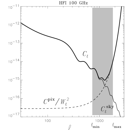
Figure 1: The simulated angular power spectrum of the CMB and pixel noise for the Planck HFI 100 GHz channel. The solid curve is the power spectrum $C_{\ell}^{\rm sky}$, which includes the CMB signal and foregrounds, and the dash line is the de-convolved noise power spectrum $C^{\rm pix}/W_{\ell}^{2}$. The thick curve represents the de-convolved power spectrum of the combined signal $C_{\ell}$. The shaded area shows the optimal top-hat filtering range $(\ell_{\min},\ell_{\max})$ for this channel, taken from Chiang et al. (2002b). We can see from the figure that $C_{\ell}(\ell_{\max})\simeq C^{\rm pix}/W^{2}(\ell_{\max})$ and $C_{\ell}(\ell_{\min})\simeq C^{\rm sky}(\ell_{\min})$.

As one can see from Eq. (45) these perturbations correspond to $||f(\ell)||\gg||F(\ell)||$ at the ranges $k_{\max}-\delta k_{\max}\leq k\leq k_{\max}$ and $k_{\min}-\delta k_{\min}\leq k\leq k_{\min}$. Thus finding the optimal values of the $k_{\min}$ and $k_{\max}$ parameters through the same treatment as in the last section is not appropriate. From a theoretical point of view that means that for a given top-hat shape of the filter the point of maxima of the gain parameter does not correspond to any solutions for Eq. (34).

In order to find the optimal $k_{\min}$ and $k_{\max}$ values we use instead the following conditions $\partial R(k_{\min},k_{\max})/\partial k_{\min}=0$ and $\partial R(k_{\min},k_{\max})/\partial k_{\max}=0$. For Eq. (44) these conditions lead to

$$2\overline{B}(k_{\max})\int\limits_{\textstyle k_{\min}}^{\textstyle k_{\max}}dk\;k\;W^{2}(k)C(k)$$ (46)

$$= W^{2}(k_{\max})C(k_{\max})\int\limits_{\textstyle k_{\min}}^{\textstyle k_{\max}}dk\;k\;\overline{B}(k),$$

and

$$2\overline{B}(k_{\min})\int\limits_{\textstyle k_{\min}}^{\textstyle k_{\max}}dk\;k\;W^{2}(k)C(k)$$ (47)

$$= W^{2}(k_{\min})C(k_{\min})\int\limits_{\textstyle k_{\min}}^{\textstyle k_{\max}}dk\;k\;\overline{B}(k).$$

We get from Eq. (46) and Eq. (47)

$$W^{2}(k_{\min})C(k_{\min})=\frac{\overline{B}(k_{\min})}{\overline{B}(k_{\max})}W^{2}(k_{\max})C(k_{\max}).$$ (48)

Apart from a trivial solution in Eq. (48), with undefined value of the $\overline{k}=k_{\max}=k_{\min}$, there are non-trivial solutions. For comparison with other filters we use the same circular Gaussian model for the antenna beam and the window function, $W^{2}(k)=\overline{B}^{2}(k)=\exp(-k^{2}\theta_{B}^{2})$, where $\theta_{B}$ is the ${\rm FWHM}/\sqrt{8\ln 2}$, so from Eq. (48) we have $\overline{B}(k_{\max})C(k_{\max})=\overline{B}(k_{\min})C(k_{\min})$. We can assume that $k_{\min}\theta_{B}<1$,

$$\overline{B}(k_{\min})=\exp(-k_{\min}^{2}\theta^{2}_{B}/2)\simeq 1\gg\exp(-k_{\max}^{2}\theta^{2}_{B}/2).$$ (49)

Figure 2: The point source extraction rate from the TOF and the ATHF. We put 50 point sources with $1.5\sigma_{\rm CMB}$ randomly in the CMB map simulating the Planck HFI 100 GHz channel with the corresponding pixel noise. This number of point sources is too large for the 100 GHz frequency channel, it nevertheless serves as the efficiency (percentage) of extraction rate. The elliptical beam is rotating across the simulation patch with ellipticity ratio $\theta_{+}/\theta_{-}=1.3$. The plot is the extraction percentage of point sources against the $\theta$ inserted to the TOF (in terms of $\theta_{0}=10.7/\sqrt{8\ln 2}$ (arcmin) ). In the dotted curve, the power spectrum is precisely known. The short-dash curve is the case when the slope of the CMB power spectrum has 5 per cent more tilt, whereas the long-dash line 5 per cent less tilt. The horizontal level marks the ATHF extraction percentage. With the exact power spectrum, the TOF is still able to detect 85 per cent of the point sources if the supplied $\theta$ is chosen in between $\theta_{+}$ and $\theta_{-}$.

We further have the following two assumptions. At the range of $k\la k_{\min}$, the power spectrum of the combined signal $C(k_{\min})$ is mainly determined by the sky signals, and the pixel noise contribution is not significant, so

$$C(k_{\min})\simeq C^{\rm sky}(k_{\min}).$$ (50)

On the other hand, for the range of $k\ga k_{\max}$, the power spectrum is mainly determined by the pixel noise power spectrum, which leads

$$C(k_{\max})\simeq\frac{C^{\rm pix}}{W^{2}(k_{\max})}.$$ (51)

The assumptions of Eq. (49), (50) and (51) are illustrated in Fig. 1, in which we show the simulated power spectrum for the Planck High Frequency Instrument (HFI) 100 GHz frequency channel. Eq. (50) and Eq. (51) lead to the following relationship between $k_{\max}$ and $k_{\min}$ parameter,

$$\overline{B}(k_{\max})\overline{B}(k_{\min})=\frac{C^{\rm pix}}{C^{\rm sky}(k_{\min})},$$ (52)

which leads to

$$k_{\max}^{2}\simeq\frac{2}{\theta^{2}_{B}}\ln\left[\frac{C^{\rm sky}(k_{\min})}{C^{\rm pix}}\right].$$ (53)

The ratio $R$ can then be obtained from Eq.(44)

$$R^{\rm ATHF}\simeq g^{2}\sum_{i}S_{i}^{2}\frac{2}{\theta^{2}_{B}C^{\rm sky}(k_{\min})}.$$ (54)

We can further solve Eq. (47) by inserting Eq. (27), which then becomes (with the integral part of $C^{\rm pix}\ll C^{\rm sky}W^{2}$)

$$\int^{k_{\max}}_{k_{\min}}dk\;k\;C^{\rm sky}(k)W^{2}(k)\simeq\frac{C^{\rm sky}(k_{\min})}{2\theta^{2}}.$$ (55)

If the $C^{\rm sky}(k)=Ak^{-n}$, Eq. (55) can be approximated and we reach

$$k_{\max}\sim k_{\min}+\frac{1}{k_{\min}\theta^{2}}.$$ (56)

Note that we use the simple trapezoidal rule for the integration, which works better when the index $n$ is smaller.

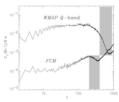
Figure 3: The power spectrum of the foreground-cleaned map by Tegmark, de Oliveira-Costa & Hamilton (2003) and the WMAP Q-band map. The shaded areas are the filtering ranges of the ATHF for point source detection: $(\ell_{\min},\ell_{\max})=(200,400)$ for the FCM and $(400,900)$ for the WMAP Q-band map.

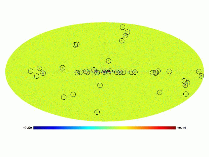
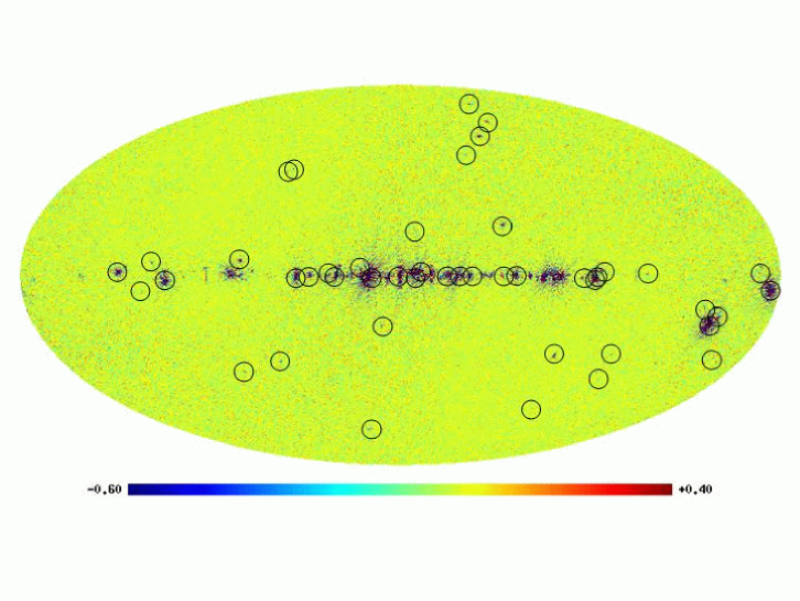
Figure 4: The adaptive top-hat filtered maps from the foreground-cleaned map (top) by Tegmark, de Oliveira-Costa & Hamilton (2003) and the WMAP Q-band map (bottom). The filtering ranges for both maps are shown in Fig. 3. In the top panel, the circled are peaks with amplitudes above $5\sigma_{\rm f}$ after filtering, which are the point source residues from the component separation. One interesting feature is that not all the residues we recover are extragalactic point sources. The dash circles are not peaks, but dips. In the bottom panel we retain the positions of the circles for comparison, from which those peaks are point sources. This is to prove that most of the peaks we retrieve from the FCM are point source residues.

4 Application of the ATHF on simulations and WMAP data

4.1 Simulations of the Planck HFI 100 GHz channel

We carry out the simulations of the Planck HFI 100 GHz channel for point source extraction by the TOF and the ATHF. The simulation area is 25.6 ${\rm deg}^{2}$, and the pixel size is 3.0 arcmin. The $\sigma_{\rm CMB}$ and the $\sigma_{\rm pix}$ are $4.03\times 10^{-5}$ and $6.07\times 10^{-6}$, respectively. Point sources with amplitudes above $2\sigma_{\rm CMB}$ at this channel would be flushed out by both (symmetric) filters with the 5 $\sigma$ criterion (see the 5th column of Table 3 in Chiang et al. [Chiang et al. 2002b]), so we add randomly 50 point sources whose amplitudes are $1.5\sigma_{\rm CMB}$ to check the efficiency. Obviously the number of point sources is too large for this frequency channel, but it serves as the demonstration of the efficiency of extraction. We specifically use an elliptical beam shape in the simulation with ellipticity ratio $\theta_{+}/\theta_{-}=1.3$ [Burigana et al. 1998]. We designate the elliptical beam size such that $\theta_{-}^{2}+\theta_{+}^{2}=2\theta_{0}^{2}$ where $\theta_{0}={\rm FWHM}/\sqrt{8\ln 2}$. For the HFI 100 GHz channel the FWHM is 10.7 arcmin. In order to simulate more realistic situations, we put this beam in rotation while scanning across the simulation area in order to investigate how the elliptical beam could affect the efficiency of point source extraction for the TOF and the ATHF.

The period of rotation of the beam is $2\pi$ along both sides of the simulation square. Although the rotation period is too large for such size of map, it nevertheless can elucidate the effect of elliptical beam shape regarding point source extraction.

Without the exact information of the in-flight beam size and orientation, the optimal form of the TOF is by inserting a circular beam function into Eq. (41), where the window function $W^{2}_{k}=\overline{B}_{k}^{2}=\exp(-k^{2}\theta^{2})$. In Fig. 2 we plot the point source extraction rate from the TOF for the 50 point sources. The plot is the extraction percentage of point sources against the $\theta$ inserted to the TOF (in terms of 100 GHz channel $\theta_{0}$). We would like to examine, for in-flight elliptical beam shapes, how the supplied beam function for the TOF can affect the extraction rate. In the dotted curve, the power spectrum is precisely known. The short-dash curve is the case when the slope of the CMB power spectrum has 5 per cent more tilt, whereas the long-dash line 5 per cent less tilt. The horizontal line marks the ATHF extraction percentage. With the exact power spectrum, the TOF is able to detect 85 per cent of the point sources with amplitude $1.5\sigma_{\rm CMB}$ when the supplied $\theta$ is chosen in between $\theta_{+}$ and $\theta_{-}$. For the case of 5 per cent more tilt in power spectrum, the supplied beam function will need adjustment to a smaller $\theta$ value to ensure the TOF to have a maximal resonance, and adjustment to a larger $\theta$ for the case of 5 per cent less tilt. On the other hand, the ATHF can reach 74 per cent of extraction rate without any information. From Fig. 2 it is not surprising that the ’safe bet’ of the beam function is $\theta/\theta_{0}\simeq 1$ for the uncertainties in the power spectrum. However, as the cleaning of foreground contamination precedes the determination of the angular power spectrum, and during the whole sky scan of the Planck mission, the possible degradation effect of the mirrors could change the beam size and shape, the efficiency of the TOF will be hampered.

4.2 The ATHF on the WMAP derived map

In this subsection we apply the ATHF to the derived map from the WMAP 1-year data. The derived maps are produced by Tegmark, de Oliveira-Costa & Hamilton [Tegmark, de Oliveira-Costa & Hamilton 2003] performing an independent component separation analysis from the WMAP team. They are the foreground-cleaned map (FCM) and the Wiener-filtered map (WFM). The FCM was tested to be non-Gaussian [Chiang, Naselsky, Verkhodanov & Way 2003], partly due to galactic emission. Here we investigate the possible point source residues from their component separation.

We use the ATHF on the FCM as it is the map with scientific significance. In Fig. 3 we show the power spectra of the FCM and the WMAP Q-band map with the corresponding filtering ranges (the shaded area) of the ATHF: $(\ell_{\min},\ell_{\max})=(200,400)$ for the FCM and $(400,900)$ for the WMAP Q-band map. It is easy to see that the CMB (plus foreground) power spectra (convolved with the beam) and the noise level. Note that the presentation of the angular power spectrum in Fig. 3 is the standard format, i.e. $C_{\ell}$ with the factor $\ell(\ell+1)/4\pi$, which is different from Fig. 1 used for analysis in the previous Section. We therefore apply the ATHF with filtering ranges covering the conjunction of the CMB and noise power curves. The choice of the filtering range follows the rule of the thumb described in Chiang et al. [Chiang et al. 2002b]: the $\ell_{\min}$ to exclude most of the CMB power, the $\ell_{\max}$ the noise power, and both to keep the part being convolved by the beam.

Fig. 4 shows the filtered maps of the FCM (top panel) and the WMAP Q-band map (bottom). The circled in the top panel are filtered peaks with amplitudes above $5\sigma_{\rm f}$. One interesting feature in Fig. 4 is that not all the residues we recover are extragalactic point sources. The dash circles are not peaks, but dips. In the bottom panel we retain the positions of the circles for comparison, from which those peaks are point sources. This is to prove that most of the peaks we retrieve from the FCM are point source residues. We do not intend to recover all residues from one single iteration of the ATHF but simply demonstrate the usefulness and quickness of the ATHF on the real data. Application of the ATHF on the WMAP 5 different channel maps will be on a separate paper.

One important issue related to elliptical beam-convolved point source extraction is the removal of point sources. Normally, circular Gaussian profile is used for cleaning the elliptical beam-convolved point sources from the map after detection of the point source position. Due to the ellipticity of the beam and pixel noise, there are considerable residues after the cleaning by circular Gaussian profile. To eliminate the residual peaks, we apply a simple algorithm that is modified from the so-called hybrid median filter used in signal processing. The hybrid median filter is useful in noise reduction and in particular in elimination of shot noise. This non-linear filter replaces the targeting pixel with average of the neighboring pixels from the same row, column and two diagonals. In the modified cascading version, the targeted region ($3\times 3$ pixels) centered at the residual peak is replaced with the following algorithm (see Fig. 5). The central pixel is replaced by the median of the 8 pixels from the same row, column, and two diagonals right outside the targeted region. The four pixels at the four corners in the region can then be decided by the median of their 4 corner pixels, which include the already-replaced central pixel. The rest 4 pixels can be replaced by the median of their neighbouring pixels from the same row and column.

5 Conclusions

We have discussed analytically the three main linear filters for point source extraction of the Planck mission. The TOF is optimal in terms of the gain factor. The so-called optimal pseudo-filter is at its best asymptotic at the far ends to the TOF under certain circumstance. Both of these filters require the experiment parameters such as the beam shape and size.

Note that the calculation is based on the simple geometrical model of the beam. As we mention in the beginning, the point source is the reflection of, among others, the beam shape properties. The possible antenna beam degradation would be a problem for the calibration of the in-flight antenna beam shape [Naselsky et al. 2002], causing the change of the inclination and the ellipticity ratio of the beam during the mission.

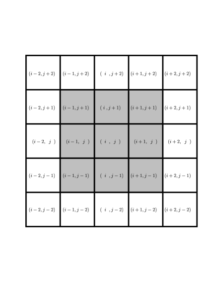
Figure 5: The cascading hybrid median filtering scheme. For a residual peak located at $(i,j)$ from the cleaning by circular Gaussian profile, we can apply the cascading hybrid median filter to replace the inner $3\times 3$ pixels. First of all, we replace the central pixel $(i,j)$ by the median of the 8 pixels from the same row, column, and the diagonals outside the targeted region, i.e., by the median of pixels $(i-2,j)$, $(i-2,j+2)$, $(i,j+2)$, $(i+2,j+2)$, $(i+2,j)$, $(i+2,j-2)$, $(i,j-2)$ and $(i-2,j-2)$. Once the central pixel is decided, we can in turn replace the four corners by the median of its diagonals, e.g., the pixel $(i+1,j+1)$ can be replaced by the median of $(i,j+2)$, $(i+2,j+2)$, $(i+2,j)$ and the replaced $(i,j)$. Then the last 4 pixels can be replaced by their neighbouring pixels of the same row and column, e.g., $(i+1,j)$ by the median of $(i+1,j+1)$, $(i+2,j)$, $(i+1,j-1)$ and the replaced $(i,j)$.

There is one comment on the extraction of point sources from the time-ordered scans when the inclination of the beam, the issue of pointing and the noise properties are most crucial: the inclination angle and the pointing will decide the point source FWHM on the time-ordered data, for which the ATHF is particularly useful.

Note also that we can easily generalize the multi-frequency method for point source extraction [Naselsky, Noviko & Silk 2002] by applying the ATHF for all Planck frequency channels.

References

- [Bardeen et al. 1986] Bardeen J. M., Bond J. R., Kaiser N., Szalay A. S., 1986, ApJ, 304, 15
- [Barreiro et al. 2003] Barreiro R.B., Sanz J.L., Herranz D., Martínez-González E., 2003, MNRAS, 342, 119
- [Bennett et al. 2003a] Bennett C. L. et al., 2003, ApJ, 583, 1
- [Bennett et al. 2003b] Bennett C. L. et al., 2003, ApJS, 148, 97
- [Bond & Efstathiou 1987] Bond J. R., Efstathiou G., 1987, MNRAS, 226, 655
- [Burigana et al. 1998] Burigana C., Maino D., Mandolesi N., Pierpaoli E., Bersanelli M., Danese L., Attolini M. R. 1998, A&AS, 130, 551
- [Burigana et al. 2001] Burigana C., Natoli P., Vittorio N., Mandolesi N., Bersanelli M., 2001, Exper. Astro., 12, 87
- [Cayón et al. 2000] Cayón L., Sanz J. L., Barreiro R. B., Martínez-González E., Vielva P., Toffolatti L., Silk J., Diego J. M., Argüeso F., 2000, MNRAS, 315, 757
- [Chiang & Naselsky 2003] Chiang L.-Y., Naselsky P.D., in preparation
- [Chiang, Naselsky, Verkhodanov & Way 2003] Chiang L.-Y., Naselsky P.D., Verkhodanov O.V., Way M.J., ApJL, 590, 65
- [Chiang et al. 2002a] Chiang L.-Y., Christensen P. R., Jørgensen H. E., Naselsky I. P., Naselsky P. D., Novikov D. I., Novikov I. D., 2002a, A&A, 392, 369
- [Chiang et al. 2002b] Chiang L.-Y., Jørgensen H.E., Naselsky, I.P., Naselsky P.D., Novikov I.D., Christensen P.R., 2002b, MNRAS, 335, 1054
- [Delabrouille, Patanchon & Audit 2002] Delabrouille J., Patanchon G., Audit E., 2002, MNRAS, 330, 807
- [Doroshkevich et al. 2003] Doroshkevich A.G., Naselsky P.D., Verkhodanov O.V., Novikov D.I., Turchaninov V.I., Novikov I.D., Christensen P.R., 2003, A&A submitted (astro-ph/0305537)
- [Fosalba, Doré & Bouchet 2002] Fosalba P., Doré O., Bouchet F. R. , 2002, Phys. Rev. D, 66, 063003
- [Gabor 1946] Gabor D., 1946, Theory of Communication, Proc. IEE., 93, 429
- [Górski, Hivon & Wandelt 1999] Górski, K. M., Hivon, E., & Wandelt, B. D. 1999, Proceedings of the MPA/ESO Cosmology Conference “Evolution of Large-Scale Structure”, eds. A. J. Banday, R. S. Sheth and L. Da Costa, PrintPartners Ipskamp, NL
- [Hansen, Gorski & Hivon 2003] Hansen F. K., Gorski K. M., Hivon E., 2003, MNRAS, 343, 559
- [Hobson et al. 1999] Hobson M. P., Barreiro R. B., Toffolatti L., Lasenby A. N., Sanz J. L., Jones A. W., Bouchet F. R., 1999, MNRAS. 306, 232.
- [Naselsky, Novikov & Silk 2002] Naselsky P. D., Novikov D., Silk J., 2002, ApJ, 565, 655
- [Naselsky, Noviko & Silk 2002] Naselsky P. D., Novikov D., Silk J., 2002, MNRAS, 335, 550
- [Naselsky et al. 2002] Naselsky P. D., Verkhodanov O. V., Christensen P. R., Chiang L.-Y., 2002, A&A submitted (astro-ph/0211093)
- [Page et al. 2003] Page L. et al., 2003, ApJS, 148, 39
- [Pierpaoli 2003] Pierpaoli E., 2003, ApJ, 589, 58
- [Sanz, Herranz & Martínez-González 2001] Sanz J. L., Herranz D., Martínez-González E., 2001, ApJ, 552, 484
- [[\citenamSlezak, Bijaoui & Mars1990] Slezak E., Bijaoui A., Mars G., 1990, A&A, 227, 301
- [Souradeep & Ratra 2001] Souradeep T., Ratra B., 2001, ApJ, 560, 28
- [Tegmark & Efstathiou 1996] Tegmak M., Efstathiou G., 1996, MNRAS, 281, 1297
- [Tegmark & de Oliveira-Costa 1998] Tegmark M. & de Oliveira-Costa A., 1998, ApJ, 500, L83
- [Tegmark, de Oliveira-Costa & Hamilton 2003] Tegmark M., de Oliveira-Costa A., Hamilton A., 2003, PRD submitted (astro-ph/0302496)
- [Vielva et al. 2001] Vielva P., Martínez-González E., Cayón L., Diego J.M., Sanz J. L., Toffolatti L., 2001, MNRAS, 326, 181
- [Vielva et al. 2003] Vielva P., Martínez-González E., Gallegos J.E., Toffolatti L., Sanz J. L., 2003, MNRAS, 344, 89
- [Vio, Tenorio & Wamsteker 2002] Vio R., Tenorio L., Wamsteker W., 2002, A&A, 391, 789
- [White & Srednicki 1995] White M., Srednicki M., 1995, ApJ, 443, 6
- [Wu et al. 2001] Wu J. H. P. et al., 2001, ApJS, 132, 1
- [Zabotin & Naselsky 1985] Zabotin N. A., Naselsky P. D., 1985, SvA, 29, 614