The galaxy population of the $z=1$ cluster of galaxies MG2016+112

Abstract

A photometric redshift analysis of galaxies in the field of the wide-separation gravitational lens MG2016+112 reveals a population of 69 galaxies with photometric redshifts consistent with being in a cluster at the redshift of the giant elliptical lensing galaxy $z=1.00$. The $Ks$-band luminosity function of the cluster galaxies is well represented by the Schechter function with a characteristic magnitude $K^{*}_{s}=18.90_{-0.57}^{+0.45}$ and faint-end slope $\alpha=-0.60^{+0.39}_{-0.33}$, consistent with what is expected for a passively evolving population of galaxies formed at high redshift, $z_{f}>2$. From the total $Ks$-band flux of the cluster galaxies and a dynamical estimate of the total mass of the cluster, the restframe $Ks$-band mass-to-light ratio of the cluster is derived to be $M/L_{Ks}=27^{+64}_{-17}\,h_{50}\,(M/L_{Ks})_{\sun}$, in agreement with the upper limit derived earlier from Chandra X-ray observations and the value derived locally in the Coma cluster. The cluster galaxies span a red sequence with a considerable scatter in the colour-magnitude diagrams, suggesting that they contain young stellar populations in addition to the old populations of main-sequence stars that dominate the $Ks$-band luminosity function. This is in agreement with spectroscopic observations which show that 5 out of the 6 galaxies in the field confirmed to be at the redshift of the lensing galaxy have emission lines. The projected spatial distribution of the cluster galaxies is filamentary-like rather than centrally concentrated around the lensing galaxy, and show no apparent luminosity segregation. A handful of the cluster galaxies show evidence of merging/interaction. The results presented in this paper suggest that a young cluster of galaxies is assembling around MG2016+112.

1 introduction

1.1 Galaxy evolution in clusters

The predominance of early-type galaxies in clusters compared with the field is a clear sign that the evolution of galaxies depends on environment, but the physical mechanism at work, in particular the question of when and how the most massive galaxies, the giant ellipticals, formed is a topic of ongoing theoretical and observational research.

The traditional “monolithic” elliptical galaxy formation scenario proposed by Eggen et al. (1962) postulates a single burst of star formation at high redshift, followed by passive stellar evolution.

Early type galaxies in nearby and intermediate redshift clusters are observed to form a tight colour-magnitude relation (Bower et al., 1992; Aragon-Salamanca et al., 1993; Gladders et al., 1998; Stanford et al., 1998), or “red sequence” which when combined with the close correlation between galaxy mass and metallicity implied by the Mg₂-$\sigma$ relation (Bender et al., 1993) is explained naturally by a single, early episode of star formation ($z_{f}>2$). If more massive galaxies are more efficient at retaining supernova ejecta, they will have higher metallicities, and therefore redder colours (Arimoto & Yoshii, 1987; Kodama & Arimoto, 1997).

There is however many pieces of evidence suggesting that the evolution of the entire cluster galaxy population is not as simple as expected from the monolithic galaxy formation scenario. The fraction of blue galaxies in clusters increase rapidly with redshift (Butcher & Oemler, 1978, 1984; Rakos & Schombert, 1995). High resolution imaging and spectroscopic studies show that a significant fraction of intermediate redshift blue galaxies are late-type spirals with emission lines and/or post-starburst signatures (Dressler & Gunn (1992); Dressler et al. (1999); Poggianti et al. (1999) and that the cluster S0 population is far less abundant at $z\sim 0.5$ than today. It has been proposed that these blue star-forming galaxies are the progenitors of cluster S0 galaxies (Dressler et al., 1997; van Dokkum et al., 1998; van Dokkum et al., 2000). In agreement with this explanation of the Butcher-Oemler effect, some S0s in the present epoch appear to contain younger stellar populations (Kuntschner & Davies, 1998).

Hierarchical structure formation models present a very different view of galaxy evolution in which galaxies assemble by merging of smaller stellar systems over a wide redshift range. In this scenario, the evolution of elliptical galaxies are governed by the time at which the bulk of the stellar populations are formed, the era when the majority of mergers took place, and the amount of new star formation induced during each merger event. If the formation of the stars in an elliptical galaxy takes place over a broad cosmic time interval, then ellipticals at any redshift should exhibit a wide range of mass-weighted stellar ages. If however most stars in present day cluster ellipticals were formed in smaller disks at high redshift $z\gg 1$ and if little additional star formation took place in subsequent mergers, then the end product ellipticals could appear to be old and approximately coeval even if the bulk of merging took place relatively late. The hierarchical models of Kauffmann & Charlot (1998a) reproduce the colour-magnitude relation of ellipticals because more massive galaxies are formed from merging of systematically more massive progenitors, which retain more metals when forming stars.

Discriminating between the two formation scenarios described above is difficult, even when studying galaxies in clusters at high redshift. An increasing number of observations (Stanford et al., 1997; Ellis et al., 1997; Stanford et al., 1998; Rosati et al., 1999; Nakata et al., 2001) show that the evolution of the “red sequence” to redshifts $z\sim 1$ is consistent with a high formation redshift and a subsequent passive evolution favored by monolithic collapse, but none of them can exclude the possibility that cluster ellipticals formed from mergers of smaller galaxies as long as the bulk of star formation took place at much larger redshifts and there was little star formation in the subsequent merging process.

One way to distinguish between the two scenarios is by studying the evolution of the mass function of the cluster galaxies. Hierarchical galaxy formation models predicts the mass assembly of galaxies to take place over a long time scale ($z\ll 2$) and to be quite decoupled from star formation (Kauffmann & Charlot, 1998b). If this picture is true, a strong evolution of the stellar mass function with redshift is expected. This evolution is best studied in the $Ks$-band because it is relatively unaffected by ongoing/recent star-formation and hence directly measures the growth of galaxy mass (Kauffmann & Charlot, 1998b).

Locally, the cluster galaxy luminosity function have been studied in great detail both at optical and Near Infrared (NIR) wavelengths. Goto et al. (2002) derive the composite luminosity function of 204 “Sloan Digital Sky Survey Cut & Enhance Galaxy Cluster Catalog” in the redshift range range $z=0.02$ to $z=0.25$ in the five SDSS bands $u^{*}$, $g^{*}$, $r^{*}$, $i^{*}$ and $z^{*}$, and find that the faint-end slope of the luminosity function becomes flatter toward the redder wavebands, consistent with the hypothesis that the cluster luminosity function has two distinct underlying populations; a population of bright ellipticals with a gaussian-like luminosity distribution that dominate the bright end, and a population of faint blue star-forming galaxies with a steep power-law like luminosity distribution, that dominate the faint-end. de Propris et al. (1998) derive the NIR (H-band) luminosity function of the Coma cluster galaxies, and find results consistent with the above picture of a population of bright red galaxies and large population of faint blue dwarf galaxies.

HST imaging of high redshift cluster galaxies have revealed a population of luminous “red” mergers in high redshift clusters (van Dokkum et al., 2000; van Dokkum et al., 2001). The existence of these galaxies which follow the same colour-magnitude relation as the cluster ellipticals (but with a slightly larger scatter) supports the hierarchical galaxy formation scenario.

The bright (massive) end of the luminosity function is expected to steepen and shift to fainter magnitudes at high redshift, as the old bright cluster galaxies begin to break up into building blocks.

In contrast to the bright cluster galaxies, the faint cluster galaxies seem to have a much greater diversity of star formation histories (Kodama & Bower, 2001). The Butcher-Oemler effect in intermediate redshift is an example of this. If this progression of activity to lower-mass galaxies as the universe ages is a consequence of the faint galaxies forming at later cosmic times than their massive counterparts, then distant clusters should have a luminosity function with a declining faint-end slope in contrast to rising faint-end slope of local clusters (de Propris et al., 1998).

The evolution of the $K$-band luminosity function in the redshift range $z=0.1$-$0.9$ has been studied by de Propris et al. (1999). The evolution of the characteristic magnitude $K^{*}$ of the galaxies, is found to be consistent with what is expected for a passively evolving population of galaxies formed at $z_{f}>2$. The data is not deep enough to constrain the faint-end slope which is fixed at $\alpha=-0.9$ (the value derived in the H-band for the Coma cluster). The authors find no significant dependence on the X-ray luminosity of the clusters.

Nakata et al. (2001) extend the study to $z=1.2$ by deriving the $K$ band luminosity function for the cluster around the radio galaxy 3C324. These authors also choose to fix the faint-end slope at $\alpha=-0.9$ and find consistency with what is expected for passively evolving stellar populations formed at $z_{f}>2$.

The suggested passive evolution of $K^{*}$ with redshift to $z=1.2$ is a nice confirmation of the passively evolving stellar population found from other methods (such as the colour-magnitude relation), but does not help discriminate between the monolithic and hierarchical formation scenarios, since no steepening of the bright end of the luminosity function (a deficit of the brightest galaxies) has been observed and no attempt has been made to measure the faint-end slope.

1.2 Previous observations of the MG2016+112 system

MG2016+112 is a wide separation gravitational lens first identified by Lawrence et al. (1984) to be comprised of at least three lensed images of an active galactic nucleus (AGN) at redshift $z=3.269$. The primary lensing object is a giant elliptical galaxy at $z=1.004$ (hereafter “the lens galaxy”, Schneider et al. (1986); Soucail et al. (2001); Koopmans & Treu (2002)). Wide separation gravitational lens systems have in many cases been found to contain galaxy clusters or groups that contribute significantly to the large separation angles. A nice property of clusters discovered in this way is that they are mass selected, and therefore not biased toward the old relaxed systems that clusters selected in X-rays or in the optical/NIR are (since their selection depends on the presence of thermalized gas and/or central concentrations of luminous old red galaxies).

Hattori et al. (1997) reported the detection of resolved X-ray emission at $z\sim 1$ centered on the lens galaxy. This result was based on the detection of an X-ray line at 3.35 keV in the ASCA spectra of the system, which was interpreted as Fe K emission originating from a cluster at $z\sim 1$, and on the detection of “diffuse” X-ray emission near the giant elliptical in ROSAT HRI observations. Infrared and optical observations of the field revealed no excess of galaxies around the giant elliptical lens (Schneider et al., 1985; Langston et al., 1991; Lawrence et al., 1993). This led to the suggestion of a “dark cluster” associated with the lens, in which a cluster sized dark matter and hot gas overdensity exists with few optically bright galaxies ($M/L_{V}>2000M_{\sun}/L_{\sun}$). This conclusion was puzzling as the observed iron line in the X-ray spectra indicated a near solar metallicity for the cluster, which implies a long history of star-formation in the region. Benítez et al. (1999) re-analyzed the ROSAT HRI data and found a faint elliptical X-ray source which was coincident with a red galaxy overdensity. Deep $V$,$I$ and $K$ band Keck imaging revealed a red sequence of galaxies, with colours consistent with being at redshift $z\sim 1$.

Soucail et al. (2001) performed a spectroscopic survey of 44 galaxies in the field and found an excess of 6 red galaxies securely identified to be at $z\sim 1$, though not very centrally concentrated around the giant elliptical galaxy. For these six galaxies a mean redshift of $z=1.005$, a velocity dispersion of $\sigma=771^{+430}_{-160}$km s^-1, a dynamical mass estimate of $2.8\times 10^{14}h_{50}M_{\sun}$ and a V-band mass-to-light ratio of $M/L_{V}=215^{+308}_{-77}h_{50}M_{\sun}/L_{\sun}$ was derived.

It is interesting to note that a high fraction of the $z=1$ galaxies (5 out of 6) have emission lines in their spectra, indicating the presence of young stellar populations. This is a much larger fraction than in low redshift clusters which are dominated by old quiescent galaxies with no emission lines, and also much higher than in other high redshift ($z\geq 1$) clusters, where the fraction of emission line galaxies is found to be 10-15% (Stanford et al., 1997; Rosati et al., 1999).

Clowe et al. (2001) performed a weak lensing analysis of the field and detected a mass concentration 64″ northwest of the lensing galaxy, and were able to rule out (at the $2\sigma$ level) a mass peak centered on the lensing galaxy of the size suggested by the Hattori et al. (1997) X-ray observations.

Chartas et al. (2001) recently acquired a 7.7 ksec observation of the system with Chandra. These observations can account for all the X-ray emission as originating from the lensed images and additional X-ray point sources in the field, and place an $3\sigma$ upper limit on the 2-10 keV flux and luminosity of diffuse cluster emission of 1.6 $\times$ 10^-14 ergs s^-1 cm^-2 and 1.7 $\times$ 10⁴⁴ ergs s^-1, respectively, and an estimated upper limit on the mass $M_{500}<4.5\times 10^{14}h_{50}M_{\sun}$ and mass-to-light ratio of $M/L_{V}<190M_{\sun}/L_{\sun}$.

Rather than being an X-ray luminous “dark-cluster”, MG2016+112 thus turned out to be a spectroscopically confirmed cluster of galaxies, detected neither in X-rays nor in weak lensing maps.

In this paper we revisit the system through deep NIR and optical observations. We identify 69 galaxies in the field with photometric redshifts consistent with being cluster galaxies at redshift $z=1$ and derive their colour-magnitude sequences and their luminosity function.

The outline of the paper is as follows: In section 2 we describe the observations and data reduction. In section 3 we describe the construction of a multi colour photometric catalog of galaxies in the field (object detection, matching, photometry, star/galaxy separation). In section 4 we discuss the photometric redshift analysis. The results are presented in section 5 and summarized in Section 6.

Throughout this paper we assume a flat $\Omega_{\Lambda}=0.3$, $\Omega_{\Lambda}=0.7$, $h_{0}=0.70$ cosmology unless otherwise noted.

2 Observations and data reduction

The observational basis of this work consists of very deep NIR $J$ and $Ks$ band observations carried out with the ISAAC instrument (proposal 63.O-0379) in service mode between May and July 1999, and moderately deep optical $B$, $V$, $R$, and $I$ band observations carried out with the FORS1 instrument (proposal 65.O-0666) in service mode in July 2000. Both FORS1 and ISAAC are mounted on the VLT/ANTU telescope. ISAAC employs a $1024^{2}$ Hawaii array, with a pixel scale of $0\aas@@fstack{\prime\prime}147$ and a field of view (FOV) of $2\aas@@fstack{\prime}5\times 2\aas@@fstack{\prime}5$. FORS1 employs a $2048^{2}$ CCD (TK2048EB4) which with the high resolution collimator used for the present observations has a pixel scale of $0\aas@@fstack{\prime\prime}1$ and a FOV of $3\aas@@fstack{\prime}4\times 3\aas@@fstack{\prime}4$.

The data was originally obtained for other purposes than studying the cluster galaxy population. The NIR dataset was designed to perform a weak lensing analysis on the background galaxies. The optical dataset was designed to study the central bright gravitationally lensed QSO and is therefore not deep enough to detect the fainter cluster galaxies. The derived magnitudes (or upper limits) however serve as powerful input for the photometric redshift analysis which separates the cluster galaxies from the foreground and background field galaxy population. All observations were performed in excellent seeing conditions. The observing log is given in Tab. 1.

Table 1: Log of the VLT/UT1 observations

Instrument	Filter	NExp	Exp	Seeing	Completeness
ISAAC	$Ks$	275	60	0$\aas@@fstack{\prime\prime}$4	22$\aas@@fstack{m}$0
ISAAC	$J$	70	120	0$\aas@@fstack{\prime\prime}$4	23$\aas@@fstack{m}$0
FORS1	$I$	2	200	0$\aas@@fstack{\prime\prime}$4	24$\aas@@fstack{m}$0
FORS1	$R$	2	150	0$\aas@@fstack{\prime\prime}$4	24$\aas@@fstack{m}$5
FORS1	$V$	4	180	0$\aas@@fstack{\prime\prime}$4	26$\aas@@fstack{m}$0
FORS1	$B$	5	300	0$\aas@@fstack{\prime\prime}$5	27$\aas@@fstack{m}$0

NExp: number of exposures, Exp: exposure time in seconds

2.1 Reduction and calibration of NIR data

The deep near-infrared imaging consists of 70 images of 2 minutes integration time (2 hours 20 minutes) obtained in $J$ in 3 independent sequences, and 275 images of 1 minute each (4 hours 35 minutes) obtained in $Ks$ in 5 sequences. Some of them were taken in photometric conditions while others not, so subsequent re-scaling to the photometric ones was applied in the final combination. Data reduction was performed with the “eclipse” software package (Devillard, 1997) and IRAF routines. Flat-fields were produced from series of twilight sky flats. To take into account the rapidly varying NIR background the sky value in each pixel was calculated as a running median of the pixel value in the exposures taken immediately before and after a given exposure.

To compensate for the dithering pattern and optical distortion the individual frames were transformed to a reference frame using a 3rd order geometrical transformation calculated from the position of 30-40 stars in each frame. Finally, the images were averaged with some clipping to remove residuals defects. Photometric calibration was obtained through the observations of standard calibration stars during the photometric nights of the programme.

2.2 Reduction and calibration of optical data

The individual optical data frames were bias subtracted and flat fielded using the standard ESO pipeline and cleaned for cosmic rays using Laplacian edge detection (van Dokkum, 2001). In some of the frames the background was found to have large scale gradients over the field. To properly account for this we ran all the frames through the SExtractor software (Bertin & Arnouts, 1996) with options set to save a full resolution interpolated background map, which was then subtracted from the science frames (large scale background variation are well modeled by SExtractor). Cosmetic defects in areas with no objects were patched by interpolation of the background in surrounding annuli. This was necessary since some wavebands had too few exposures for deviant pixel rejection. Finally the individual frames were geometrically transformed to the same reference frame and combined using the IRAF tasks geoform, geotran and imcombine.

The combined frames were calibrated using the atmospheric extinction and color corrected zero-points quoted on the ESO webpage, and corrected for Galactic extinction using the parameterization of the Galactic extinction law of Cardelli, Clayton & Mathis (1989), assuming the mean Galactic value for the total-to-selective extinction in the V band $R_{V}=\left<R_{V}\right>_{MW}=3.1$ and E(B$-$V)=0.22 (from interpolation of DIRBE/IRAS dust maps, Schlegel et al. 1998). Finally, all the frames were WCS calibrated using the USNO-A2.0 catalog (Monet & et al., 1998).

3 Object detection, Photometry and Matching

Object detection was done in the $Ks$ band, using the SExtractor software (Bertin & Arnouts, 1996) with default parameter settings. We searched for the detected objects in the remaining frames using the SExtractor ASSOC option, which assumes that the frames being matched have been registered to the same pixel coordinate system.

The transformations of the combined images to the $Ks$-band image were derived using the IRAF tasks geoform.

Transforming the optical images to the $Ks$-band image includes a rebinning (due to the different pixel scales of the two instruments) in addition to the distortion transformation. To avoid this image degradation, as well as other potential problems associated with non-linear image transformations, such as blurring of persistent bad pixels and cosmic ray events, corruption of the background statistics etc. we transformed the $Ks$-band object list xy-pixel coordinates to match the reference frames of the other images using the IRAF task geoxytran, rather than transforming the images themselves. In this way the photometry is performed on the original, untransformed images.

For the total $Ks$ band magnitudes of the objects we used SExtractors mag_best which has been shown to be accurate to about $0\aas@@fstack{m}05$ (Smail et al., 2001) and colours were derived in fixed apertures of approximately 12 kpc at $z=1$ (10 pixels in the ISAAC images, 15 pixels in the FORS1 images).

3.1 Completeness

To estimate the completeness magnitude of the observations we ran SExtractor object detection independently on all the frames. In Fig. 1 we plot the number of detected objects as a function of $Ks$ and $J$ band magnitude. From visual inspection of the turnover magnitudes of the distributions in Fig. 1 we estimate that the $Ks$ band observations are complete to about 22$\aas@@fstack{m}$0 and the $J$ band observations are complete to about 23$\aas@@fstack{m}$0. The estimated completeness magnitudes of all the wavebands, including the optical are listed in Tab. 1.

Figure 1: Binned representation (binsize is $0\aas@@fstack{m}5$) of the number of detected objects as a function of magnitude in the $Ks$ (full curve) and $J$ band (dashed curve). The data are estimated to be complete to $Ks$=22$\aas@@fstack{m}$0 and $J$=23$\aas@@fstack{m}$0

3.2 Star/galaxy separation

SExtractor assigns to each object a parameter class_star which ranges from 0 to 1. When the FWHM is well determined stars obtain values close to 1, while extended objects obtain values close to 0. A main concern is contamination of the galaxy sample by stars, especially since some of them (e.g. M stars) would have the same colours as early-type galaxies at the cluster redshift. We therefore adopt a very conservative threshold in the class_star parameter of 0.05. Objects with class_star larger than this value in the $Ks$ band or $J$ band are labeled stars. Now we can construct a multi colour catalogue of galaxies consisting of objects which (i) have $Ks\leq 22$ (ii) are detected in at least two bands and (iii) are classified as a galaxy by means of the class_star parameter.

4 Photometric Redshift Analysis

To separate the cluster galaxies from the foreground and background galaxies we estimated their redshifts using the public hyperz photometric redshift code of Bolzonella et al. (1996). The code uses the GISSEL98 (Galaxy Isochrone Synthesis Spectral Evolution Library) spectral evolution library of Bruzual & Charlot (1993) to build synthetic spectra with 7 different star formation histories which match the observed properties of local galaxies from E to Irr type: a constant star-forming rate and six exponentially decaying star formation rates with time scales from 1-30 Gyr. The models assume solar metallicity and a Millar-Scalo IMF, and internal reddening is considered using the Calzetti et al. (2000) model with $A_{V}$ varying between 0$\aas@@fstack{m}$0 and 1$\aas@@fstack{m}$2. Objects not detected in a waveband are assigned zero flux (with an error corresponding to the limiting magnitude) rather than just ignored in the fit. This “upper limit” is important for the photometric redshift determination and is the reason for including the rather “shallow” optical data in the analysis. Fig. 2 shows a histogram of the derived photometric redshifts of all the galaxies in the field. There is a distinct peak at redshift $z_{phot}\sim 1$, and quite a few galaxies with $z_{phot}\la 0.2$.

Figure 2: Photometric redshifts distribution of the galaxies in the field of MG2016+112 derived using hyperz.

Figure 3: Photometric redshifts of all galaxies in the field of MG2016+122 versus their $Ks$ band magnitudes. The error bars are 1$\sigma$ from hyper-z. The squares mark galaxies which have been spectroscopically confirmed to be at redshift $z=1$ (Soucail et al., 2001)

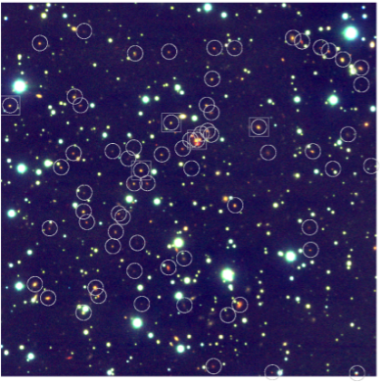
Figure 4: Composite $Ks$, $Js$, $I$-band image of the field of MG2016+112. The field is 2.5′$\times$2.5′. The pixel scale is $0\aas@@fstack{\prime\prime}147\,$pix^-1. The circles mark the 69 “photometric members” of the cluster at $z=1$. The squares mark the “spectroscopic members” of the cluster. North is up, East is to the left.

Figure 5: Simulated fraction of redshift $z=1$ galaxies with derived photometric redshifts in the range $0.7<z_{phot}<1.2$ as a function of $Ks$ band magnitude

In Fig. 3 we plot the derived photometric redshifts of all the galaxies in the field versus their $Ks$-band magnitude. The open squares mark the galaxies which have been spectroscopically confirmed to be at redshift $z=1$ (hereafter spectroscopic members, Soucail et al. (2001)). The full line marks the redshift of the lensing galaxy at $z=1$ while the dashed lines are the limits $z_{phot}=0.7$ and $z_{phot}=1.2$ that encompasses all the galaxies in the peak around $z_{phot}=1$, including the 5 spectroscopically confirmed ones. Fig. 3 reveals that most of the $z_{phot}\la 0.2$ are faint $Ks>20$ galaxies which may have been misclassified as dusty low redshift galaxies due to poor photometry.

We classify the 69 galaxies within the limits $0.7\leq z_{phot}\leq 1.2$ as probable cluster galaxies (hereafter photometric members). The choice of limits is a trade off between maximum cluster galaxy completeness and minimum contamination from field galaxies. We choose the lower limit to be $z_{phot}>0.7$ rather than e.g. $z_{phot}>0.8$ to avoid excluding spectroscopic members, and other cluster galaxies with similar colours. Young stellar populations in the cluster galaxies can influence their broadband colours and derived photometric redshifts due to the discrete nature of the spectral library used by hyperz. Since a large fraction of the spectroscopically confirmed cluster galaxies show evidence of recent star formation it is likely that this is also the case for other cluster galaxies. Some galaxies in the $0.7<z_{phot}<0.8$ interval may be truly foreground, but many could also be cluster galaxies at $z=1$ with recent star formation. To test the stability of the photometric redshifts derived with hyperz versus the photometric errors we did the following: For each $\Delta m$=0.5 mag bins in the observed range of magnitudes $Ks=16-22$, we generated a catalogue of 1000 galaxies at $z=1$ for the same bandpasses and limiting magnitudes as for the data of MG2016+112. The catalogue was generated using the make_catalog code in the hyperz package. The galaxies are randomly drawn from the 7 template spectral types (E to Im) used for estimating the photometric redshifts. We then apply hyperz to the catalog to estimate the photometric redshifts. In Fig. 5 we plot the fraction of the input ($z=1$) galaxies that have derived photometric redshifts in the range $0.7<z_{phot}<1.2$ as a function of $Ks$-band magnitude. From this figure it can be seen that hyperz recovers 100% of the galaxies down to magnitudes of $Ks=18.5$. At $Ks=20$ it recovers about 90% and at $Ks=22$ the recovery rate is down to 40%.

The redshift evolution of the field galaxy luminosity function, and its cosmic variance is not known with sufficient accuracy to correctly incorporate the effects of pollution from field galaxies in the completeness function analysis. Instead we will return to the issue of field contamination in Sec. 5.1 where we discuss the derived projected spatial distribution of the cluster galaxies, and in Sec. 5.4 where we discuss their luminosity function.

5 Results

5.1 Distribution of the cluster galaxies

The distribution of the cluster galaxies (photometric members) on the sky is not very centrally concentrated. This is illustrated in Fig. 4 where the overlay circles mark the photometric cluster members, and in Fig. 6 where the overlay represents contours of the smoothed density distribution of the photometric member galaxies. The contours are 3-30$\sigma$ above the background density which is taken to be the density of galaxies in the HDFN with $K_{s}<22$ and $0.7<z_{phot}<1.2$ (Fernández-Soto et al., 1999). The apparent morphology of the cluster is an elongated filamentary-like distribution similar to what is observed in other $z>1$ clusters (e.g. the Lynx clusters (Stanford et al., 1997; Rosati et al., 1999) and the RDCS J0910+5422 cluster (Stanford et al., 2002)) and consistent with what is expected for a “dynamically young” cluster in the process of assembly. The high significance of the overdensity structure, compared to the HDFN indicates that most of the photometric members are $z=1$ cluster galaxies rather than random field galaxies that would be distributed more homogeneously across the field. Fig. 7 illustrates that there is no apparent luminosity segregation of the cluster galaxies (i.e the brighter cluster galaxies are not more centrally clustered than the fainter galaxies). This is consistent with the picture of a young cluster where the smaller galaxies have not yet had time to merge and transform into the population of massive galaxies found in the center of relaxed clusters.

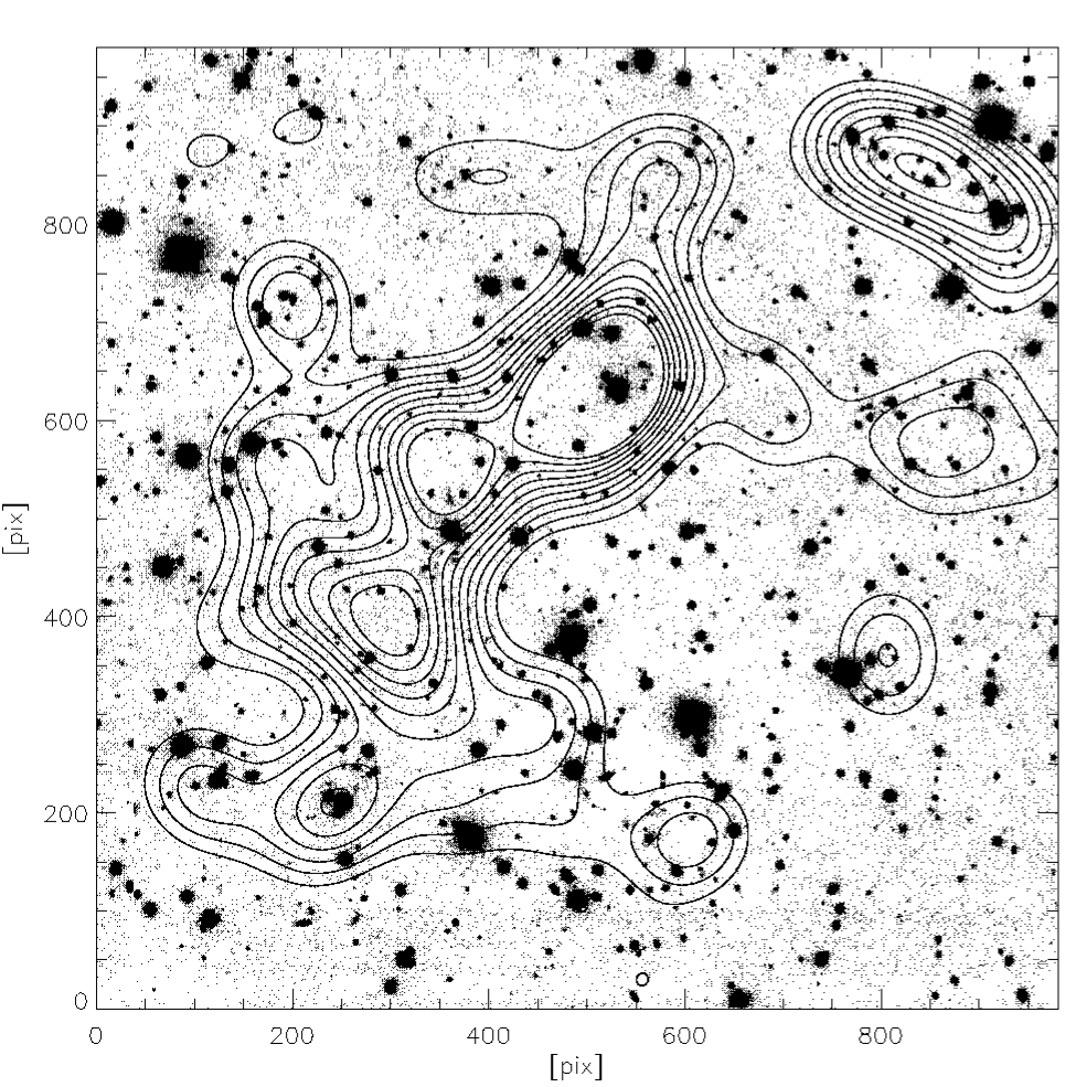
Figure 6: Contours of the smoothed density distribution of photometric member galaxies overlayed the $Ks$-band image of MG2016+112. The contours are 3-30$\sigma$ above the background density which is taken to be the density of galaxies in the HDFN with $K_{s}<22$ and $0.7<z_{phot}<1.2$ (Fernández-Soto et al., 1999). The largest concentration of photometric member galaxies is centered on the central lensing galaxy, and is part of a “loose” elongated filamentary like structure. The pixel scale is $0\aas@@fstack{\prime\prime}147\,$pix^-1. North is up, East is to the left.

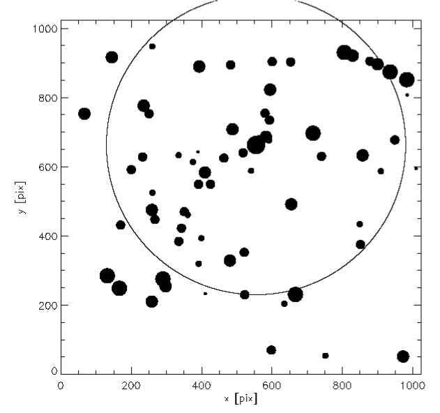
Figure 7: Distribution of the “photometric members” of the cluster at $z=1$. The area of the circles are proportional to the $Ks$-band brightness of the galaxies. The physical size of the radius of the large circle is 0.5 Mpc. The pixel scale is $0\aas@@fstack{\prime\prime}147\,$pix^-1. North is up, East is to the left.

5.2 Properties of the cluster galaxies

A full morphological analysis of the cluster galaxies requires higher resolution imaging data, and is beyond the scope of this paper, but qualitative inspection of Fig. 4 shows a wide variety of galaxies types: elliptical, spirals and even three or four mergers. Merging cluster galaxies are very rare in the cores of local relaxed clusters. The significant fraction of merging cluster galaxies found here, and in other high redshift clusters (van Dokkum et al., 2000; van Dokkum et al., 2001) is direct evidence of the hierachical formation scenario.

5.3 Colour-magnitude relation

In Fig. 8 and Fig. 9 we plot the $J-Ks$ versus $Ks$ and $R-Ks$ vs $Ks$ colour-magnitude relations of galaxies in the field of MG2016+112. Filled symbols mark galaxies within 0.5 Mpc of the lensing galaxy. We label this region the “inner region”. Open symbols mark galaxies farther away than 0.5 Mpc from the lensing galaxy. We label this region the “outer region”. The area of the outer region is approximately the same as the inner region. Also indicated are predicted colour-magnitude relations at the cluster redshift ($z=1$) for passively evolving galaxies formed at $z_{f}$=2, 3 and 5 (Kodama & Arimoto, 1997). This model assumes that the red sequence of early type galaxies in the colour-magnitude diagram is a pure metalicity sequence as a function of galaxy magnitude, and calibrate its zeropoint using the red sequence of early type galaxies in the Coma cluster.

Figure 8: $J$-$Ks$ versus $Ks$ colour magnitude relation. Squares mark spectroscopic members. Large symbols are photometric members, while small symbols are non members. Galaxies within 0.5 Mpc of the lensing galaxy are represented by filled symbols, while galaxies further away than 0.5 Mpc are represented by open symbols. The three lines are the predicted colour-magnitude relations at the cluster redshift ($z=1$) for passively evolving galaxies formed at $z_{f}$=2, 3 and 5 (Kodama & Arimoto, 1997).

Figure 9: $R$-$Ks$ versus $Ks$ colour-magnitude diagram for galaxies detected in the $R$ band. Symbols are as in Fig. 8

Most of the photometric members are concentrated in the “inner region” around the lensing galaxy, while the non members are distribubuted more homogeneously across the field. The photometric members span a “red sequence” in the colour-magnitude diagrams with a considerable scatter. The slope and zeropoint of the red sequence are hard to define due to the large scatter but are roughly consistent with predictions of the simple models.

The large observed scatter is likely to be caused by variations in the dust content, the morphology and/or the age of the stellar populations of the galaxies. The red sequence is expected to increase its scatter and eventually fall apart as the redshift approaches the formation redshift of the stars in the galaxies. The properties of the red sequence are consistent with the picture of a young cluster in the process of formation, in which the cluster galaxies habour young stellar populations and have not yet evoloved in to the old red galaxies found in the cores of relaxed clusters.

5.4 Cluster galaxy luminosity function

We can now proceed to derive the $Ks$-band luminosity function of the cluster galaxies. Since the $Ks$-band observations are complete to $Ks=22$ and we know the photometric redshift distribution of all galaxies in the field, we can do this without having to make uncertain statistical corrections to account for foreground and background contamination. To take full advantage of the data, we use a maximum likelihood technique applied directly to the luminosity distribution of the cluster galaxies, rather than doing a “least squares” fit to a binned representation. Details of the method are discussed in App.A. In Fig. 10 we show the best fitting Schechter function parameters $\alpha=-0.60^{+0.39}_{-0.33}$ and $K^{*}=18.90_{-0.57}^{+0.45}$.

Figure 10: Contour plot showing the constraints on the Schechter function parameters derived from the maximum likelihood analysis. The cross marks the best fitting parameters, the curves represents the 1-3$\sigma$ confidence levels

In Fig. 11 we plot the derived $Ks$-band luminosity function of the cluster galaxies. It is found to be well represented by the Schechter function.

Figure 11: $Ks$-band luminosity function of the cluster galaxies represented by the Schechter function with the $\alpha=-0.60^{+0.39}_{-0.33}$ and $K^{*}=18.90_{-0.57}^{+0.45}$. The filled symbols are a binned representation of the raw counts, while the open symbols have been corrected for incompleteness using the incompleteness function in Fig. 5.

The constraints on $\alpha$ are not strong, but it is important to leave it as a free parameter since the derived uncertainty on its value is coupled to the derived value of $Ks^{*}$ and its uncertainties. Also, since $\alpha$ has recently been shown to depend on wavelength (Goto et al., 2002) it is interesting to note that the value of $\alpha$ is in agreement with the value derived locally in the $z^{*}$-band (which roughly corresponds to the same restframe wavelength as the $Ks$-band at $z=1$) namely $\alpha_{z^{*},local}=-0.58$.

Earlier studies of the evolution of the luminosity function with redshift have assumed the faint-end slope to be fixed at the value measured in the Coma cluster $\alpha=-0.9$ (de Propris et al., 1999; Nakata et al., 2001). To allow a comparison with these results we repeat our analysis with the faint-end slope fixed at $\alpha=-0.9$ and derive a 1$\sigma$ constraint on the characteristic magnitude of $K^{*}_{s}=18.60^{+0.22}_{-0.24}$. In Fig. 12 we compare the derived value of $K^{*}_{s}$ with values derived at other redshifts, and with the predictions of passively evolving stellar population models with different formation redshifts (Kodama & Arimoto, 1997). Dashed lines are calculated in a $\Omega_{m}=0.3$, $\Omega_{\Lambda}=0$, $h_{0}=0.6$ cosmology while full lines are calculated in a $\Omega_{m}=0.3$, $\Omega_{\Lambda}=0.7$, $h_{0}=0.7$ cosmology. The filled circle is the value derived with $\alpha$ left as a free parameter. The open circle is the value derived with a fixed $\alpha=-0.9$. We have included this result in the plot to make a more direct comparison with results from the literature.

Figure 12: Evolution of $K^{*}_{s}$ with redshift. The curves represent the evolution predicted by stellar population synthesis models (Kodama & Arimoto, 1997), normalized to the Coma cluster which has $K^{*}_{s}=10.9$ (de Propris et al., 1998). Dashed lines are calculated in a $\Omega_{m}=0.3$, $\Omega_{\Lambda}=0$, $h_{0}=0.6$ cosmology while the full lines calculated in a $\Omega_{m}=0.3$, $\Omega_{\Lambda}=0.7$, $h_{0}=0.7$ cosmology. Lines are labeled according to the formation redshift of their stellar populations. The lines labeled “No-evolution” only include K-corrections. The circles are the results of the present work. The filled circle is the result derived with $\alpha$ as a free parameter, while the open circle is the result obtained with a fixed $\alpha=-0.9$. The diamonds and the square are results from the literature (de Propris et al., 1999; Nakata et al., 2001)

As expected from Fig. 10, fixing $\alpha$ results in a brighter best fitting $K^{*}_{s}$ with smaller errorbars, bringing it into perfect agreement with the results of de Propris et al. (1999) and Nakata et al. (2001) and consistency with what is expected for a passively evolving stellar populations formed at high redshift $z_{f}\geq 2$.

To investigate the effects of field galaxy polution we redid the analysis on a subsample of the photometric member galaxies with photmetric redshifts in the range $0.9<z_{phot}<1.1$. This limits the effects of field galaxy polution but also excludes several known (bright) cluster galaxies from the sample. The best fitting values obtained in this way are $\alpha=-0.51^{+0.43}_{-0.28}$ and $K^{*}_{s}=19.10_{-0.25}^{+0.77}$. The favored $K^{*}_{s}$ is a bit fainter, due to the exclusion of some of the brightetest galaxies from the sample, but apart from that the main effect is an increase of the size of the error bars. With the faint-end slope fixed at $\alpha=-0.9$, the best fitting characteristic magnitude hardly changes. The derived value is $K^{*}_{s}=18.55_{-0.27}^{+0.24}$.

From the present analysis we conclude that the effects of field galaxy polution on the derived luminosity function paramenters are marginal, but that fixing the faint-end slope of the cluster galaxy luminosity function directly affects the derived characteristic magnitude. We find no evidence for a steepening or shift to fainter magnitudes of the bright end of the (cluster galaxy) luminosity function at $z=1$, when compared to the local ($z=0$) one. Nor do we find a significant change of its faint-end slope to support the hierachical formation scenario.

5.5 Mass-to-light ratio

The restframe $K_{s}$-band mass-to-light ratio of the cluster around MG2016+112 can be estimated by comparing the total cluster mass, estimated from the velocity dispersion of 6 cluster members (Soucail et al., 2001), with the total K-corrected $Ks$-band flux of the cluster galaxies. We calculate the absolute K-corrected $Ks$-band magnitude of the cluster galaxies to be

$$M_{Ks}=m_{Ks}-5\,{\rm{log}}\,d_{L}-25-k_{Ks}(z=1),$$ (1)

where $d_{L}$ is the luminosity distance in Mpc calculated in a $\Omega_{m}=1$, $\Omega_{\Lambda}=0$, $h_{0}=0.5$ (for easier compariason to previous results), and $k_{Ks}(z=1)=-0.352$ is the k correction in the $Ks$ band for an object at redshift $z=1$ from Poggianti (1997) (we apply this term to be able to compare with the absolute $Ks$-band magnitude of the sun. We assume $M_{V\sun}=4.8$ and $(V-Ks)_{\sun}=1.45$).

The derived $Ks$-band mass-to-light ratio of the cluster is found to be $M/L_{Ks}=27^{+64}_{-17}\,h_{50}\,(M/L_{Ks})_{\sun}$. This is in agreement with the upper limit on the total mass of the cluster derived from X-rays (Chartas et al., 2001) which when combined with our estimate of the total $Ks$-band luminosity of the cluster galaxies translates into the following upper limit on $Ks$-band mass-to-light ratio $M/L_{Ks}<43\,h_{50}\,(M/L_{Ks})_{\sun}$, and in agreement with the $Ks$-band mass-to-light ratio derived locally in the Coma cluster $M/L_{Ks}=38\pm 23\,h_{50}\,(M/L_{Ks})_{\sun}$ (Rines et al., 2001).

6 Summary

We have obtained deep NIR and optical imaging of the field around the wide separation gravitational lens MG2016+112. A photometric redshift analysis of objects in the field, reveal 69 galaxies with photometric redshifts consistent with being in a cluster at the redshift of the lensing galaxy $z=1$.

The $Ks$-band luminosity function of the cluster galaxies is well represented by the Schechter function. The best fitting faint-end slope $\alpha=-0.60^{+0.39}_{-0.33}$ is consistent with what is measured at the same restframe wavelength (the $z^{*}$ band) locally, providing no evidence of evolution. In the bright end no steepening or shift to fainter magnitudes of the luminosity function is found. The best fitting characteristic magnitude $K^{*}=18.90_{-0.57}^{+0.45}$ is consistent with what is expected for a passively evolving population of galaxies formed at high redshift $z_{f}\geq 2$. From the $Ks$-band flux of the cluster galaxies and the total cluster mass estimates of Soucail et al. (2001) a $Ks$-band mass-to-light ratio of $M/L_{Ks}=27^{+64}_{-17}\,h_{50}\,(M/L_{Ks})_{\sun}$ is derived, consistent with the upper limit derived from Chandra X-ray observations (Chartas et al., 2001) and the value measured locally in the Coma cluster (Rines et al., 2001).

The projected spatial distribution of the cluster galaxies is filamentary-like rather than centrally concentrated around the lensing galaxy, and show no apparent luminosity segregation. A handful of the cluster galaxies shows evidence of merging and interaction. The cluster galaxies span a red sequence with a considerable scatter in the colour-magnitude diagrams, suggesting that they contain young stellar populations in addition to the old populations of main sequence stars that dominate the $Ks$-band luminosity function. This is in agreement with spectroscopic observations which show that 5 out of 6 galaxies at the redshift of the lensing galaxy has emission lines.

The evidence presented here suggest that a young cluster of galaxies is in the process of assembling around the massive lensing galaxy MG2016+112. The cluster is mass-selected (from the precence of the wide-seperation gravitationally lensed QSO) and is therefore likely to be more typical of the $z\simeq 1$ cluster population than clusters selected using X-ray or optical techniques that rely on the presence of a relaxed intra cluster medium and/or a central concentration of old bright red galaxies for the clusters to be detected.

Appendix A Deriving the Cluster Galaxy Luminosity Function using the Maximum Likelihood technique

To take full advantage of the data, we apply the maximum likelihood technique of Schechter & Press (1976) directly to the luminosity distribution of the cluster galaxies, rather than doing a “least squares” fit to a binned representation. In this way we include the information that in many magnitudes intervals no galaxies are found, and we do not make the erroneous assumption of the $\chi^{2}$ method that the underlying distribution is gaussian (it is in fact poissonian, either a galaxy is there or it is not). This in turn leads to results with more realistic errorbars.

In the magnitude interval between $m$ and $m+dm$, the expected number of galaxies $p(m)dm$ is taken to be

$$p(m)dm=f(m)n^{*}\left[10^{0.4(m^{*}-m)}\right]^{\alpha+1}e^{-10^{0.4(m^{*}-m)}}dm,$$ (2)

where $m^{*}$ is the characteristic magnitude of the cluster galaxies, $\alpha$ is the slope of the faint-end of the cluster galaxy luminosity function, $n^{*}$ is a normalization constant and $f(m)$ is the completeness function of the “photometric member” sample (shown in Fig. 5) evaluated in $m$.

Poisson statistics gives the probability that a cluster of galaxies characterized by $n^{*}$, $m^{*}$ and $\alpha$ will yield the data set actually observed ($N$; $m_{1}$,$m_{2}$,….,$m_{N}$; $m_{lim}$)

$$P={\rm{exp}}\left[\int_{-\infty}^{m_{lim}}p(m)dm\right]\prod_{i=1}^{N}\left[p(m_{i})dm\right],$$ (3)

where $m_{lim}$ is the magnitude limit (to which the dataset is complete, in this case $m_{lim}=K_{lim}=22$). The parameters $\alpha$ and $m^{*}$ which are “most likely” to represent the observed data set are those that minimizes the C statistics (the likelihood function (Cash, 1979))

$$C=-2{\rm{ln}}(P).$$ (4)

The minimum value of the C statistics $C_{min}$ is found by varying $\alpha$ and $m^{*}$. For each combination of $\alpha_{i}$ and $m_{*,i}$ we calculate the term $\Delta C=C(\alpha_{i},m_{*,i})-C_{min}$, which is distributed as $\chi^{2}$ with 2 degrees of freedom (Cash, 1979). From $\Delta C$ the 1-3$\sigma$ confidence levels can be derived in a straight forward manner as these (as for the $\chi^{2}$ distribution) are found where $\Delta C=2.29575,6.18008,11.8291$.

References

- Aragon-Salamanca et al. (1993) Aragon-Salamanca A., Ellis R. S., Couch W. J., Carter D., 1993, MNRAS, 262, 764
- Arimoto & Yoshii (1987) Arimoto N., Yoshii Y., 1987, A&A, 173, 23
- Bender et al. (1993) Bender R., Burstein D., Faber S. M., 1993, ApJ, 411, 153
- Benítez et al. (1999) Benítez N., Broadhurst T., Rosati P., Courbin F., Squires G., Lidman C., Magain P., 1999, ApJ, 527, 31
- Bertin & Arnouts (1996) Bertin E., Arnouts S., 1996, A&AS, 117, 393
- Bolzonella et al. (1996) Bolzonella M., Miralles J.-M., Pell R., 1996, A&A, 363, 476
- Bower et al. (1992) Bower R., Lucey J., Ellis R., 1992, MNRAS, 254, 589
- Bruzual & Charlot (1993) Bruzual A., Charlot S., 1993, ApJ, 405, 538
- Butcher & Oemler (1978) Butcher H., Oemler A., 1978, ApJ, 219, 18
- Butcher & Oemler (1984) Butcher H., Oemler A., 1984, ApJ, 285, 426
- Calzetti et al. (2000) Calzetti D., Armus L., Bohlin R., Kinney A., Koornneef J., Storchi-Bergmann T., 2000, ApJ, 533, 682
- Cardelli et al. (1989) Cardelli J. A., Clayton G. C., Mathis J. S., 1989, ApJ, 345, 245
- Cash (1979) Cash W., 1979, ApJ, 228, 939
- Chartas et al. (2001) Chartas G., Bautz M., Garmire G., Jones C., Schneider D. P., 2001, ApJL, 550, L163
- Clowe et al. (2001) Clowe D., Trentham N., Tonry J., 2001, A&A, 369, 16
- de Propris et al. (1998) de Propris R., Eisenhardt P. R., Stanford S. A., Dickinson M., 1998, ApJL, 503, L45
- de Propris et al. (1999) de Propris R., Stanford S. A., Eisenhardt P. R., Dickinson M., Elston R., 1999, AJ, 118, 719
- Devillard (1997) Devillard N., 1997, The Messenger, 87
- Dressler & Gunn (1992) Dressler A., Gunn J. E., 1992, ApJS, 78, 1
- Dressler et al. (1997) Dressler A., Oemler A., Couch W., Smail I., Ellis R., Barger A., Butcher H., Poggianti B., Sharples R., 1997, ApJ, 490, 577
- Dressler et al. (1999) Dressler A., Smail I., Poggianti B. M., Butcher H., Couch W. J., Ellis R. S., Oemler A. J., 1999, ApJS, 122, 51
- Eggen et al. (1962) Eggen O. J., Lynden-Bell D., Sandage A., 1962, ApJ, 136, 748
- Ellis et al. (1997) Ellis R. S., Smail I., Dressler A., Couch W. J., Oemler A. J., Butcher H., Sharples R. M., 1997, ApJ, 483, 582
- Fernández-Soto et al. (1999) Fernández-Soto A., Lanzetta K. M., Yahil A., 1999, ApJ, 513, 34
- Gladders et al. (1998) Gladders M. D., Lopez-Cruz O., Yee H. K. C., Kodama T., 1998, ApJ, 501, 571
- Goto et al. (2002) Goto T., Okamura S., McKay T. A., Bahcall N. A., Annis J., Bernard M., Brinkmann J., Gómez P. L., Hansen S., Kim R. S. J., Sekiguchi M., Sheth R. K., 2002, PASJ, 54, 515
- Hattori et al. (1997) Hattori M., Ikebe Y., Asaoka I., Takeshima T., Boehringer H., Mihara T., Neumann D. M., Schindler S., Tsuru T., Tamura T., 1997, Nature, 388, 146
- Kauffmann & Charlot (1998a) Kauffmann G., Charlot S., 1998a, MNRAS, 294, 705
- Kauffmann & Charlot (1998b) Kauffmann G., Charlot S., 1998b, MNRAS, 297, L23
- Kodama & Arimoto (1997) Kodama T., Arimoto N., 1997, A&A, 320, 41
- Kodama & Bower (2001) Kodama T., Bower R. G., 2001, MNRAS, 321, 18
- Koopmans & Treu (2002) Koopmans L. V. E., Treu T., 2002, ApJL, 568, L5
- Kuntschner & Davies (1998) Kuntschner H., Davies R. L., 1998, MNRAS, 295, L29
- Langston et al. (1991) Langston G., Fischer J., Aspin C., 1991, AJ, 102, 1253
- Lawrence et al. (1993) Lawrence C. R., Neugebauer G., Matthews K., 1993, AJ, 105, 17
- Lawrence et al. (1984) Lawrence C. R., Schneider D. P., Schmidet M., Bennett C. L., Hewitt J. N., Burke B. F., Turner E. L., Gunn J. E., 1984, Science, 223, 46
- Monet & et al. (1998) Monet D., et al. 1998, in The PMM USNO-A2.0 Catalog. (1998) A catalogue of astrometric standards.
- Nakata et al. (2001) Nakata F., Kajisawa M., Yamada T., Kodama T., Shimasaku K., Tanaka I., Doi M., Furusawa H., Hamabe M., Iye M., Kimura M., Komiyama Y., Miyazaki S., Okamura S., Ouchi M., Sasaki T., Sekiguchi M., Yagi M., Yasuda N., 2001, PASJ, 53, 1139
- Poggianti (1997) Poggianti B. M., 1997, A&AS, 122, 399
- Poggianti et al. (1999) Poggianti B. M., Smail I., Dressler A., Couch W. J., Barger A. J., Butcher H., Ellis R. S., Oemler A. J., 1999, ApJ, 518, 576
- Rakos & Schombert (1995) Rakos K. D., Schombert J. M., 1995, ApJ, 439, 47
- Rines et al. (2001) Rines K., Geller M. J., Kurtz M. J., Diaferio A., Jarrett T. H., Huchra J. P., 2001, ApJL, 561, L41
- Rosati et al. (1999) Rosati P., Stanford S. A., Eisenhardt P. R., Elston R., Spinrad H., Stern D., Dey A., 1999, AJ, 118, 76
- Schechter & Press (1976) Schechter P., Press W. H., 1976, ApJ, 203, 557
- Schlegel et al. (1998) Schlegel D. J., Finkbeiner D., Davis M., 1998, ApJ, 500, 525
- Schneider et al. (1986) Schneider D. P., Gunn J. E., Turner E. L., Lawrence C. R., Hewitt J. N., Schmidt M., Burke B. F., 1986, AJ, 91, 991
- Schneider et al. (1985) Schneider D. P., Lawrence C. R., Schmidt M., Gunn J. E., Turner E. L., Burke B. F., Dhawan V., 1985, ApJ, 294, 66
- Smail et al. (2001) Smail I., Kuntschner H., Kodama T., Smith G., Packham C., Fruchter A., Hook R., 2001, MNRAS, 323, 839
- Soucail et al. (2001) Soucail G., Kneib J.-P., Jaunsen A. O., Hjorth J., Hattori M., Yamada T., 2001, A&A, 367, 741
- Stanford et al. (1998) Stanford S. A., Eisenhardt P. R., Dickinson M., 1998, ApJ, 492, 461
- Stanford et al. (1997) Stanford S. A., Elston R., Eisenhardt P. R., Spinrad H., Stern D., Dey A., 1997, AJ, 114, 2232
- Stanford et al. (2002) Stanford S. A., Holden B., Rosati P., Eisenhardt P. R., Stern D., Squires G., Spinrad H., 2002, AJ, 123, 619
- van Dokkum (2001) van Dokkum P. G., 2001, PASP, 113, 1420
- van Dokkum et al. (2000) van Dokkum P. G., Franx M., Fabricant D., Illingworth G. D., Kelson D. D., 2000, ApJ, 541, 95
- van Dokkum et al. (1998) van Dokkum P. G., Franx M., Kelson D. D., Illingworth G. D., Fisher D., Fabricant D., 1998, ApJ, 500, 714
- van Dokkum et al. (2001) van Dokkum P. G., Stanford S. A., Holden B. P., Eisenhardt P. R., Dickinson M., Elston R., 2001, ApJL, 552, L101