XMM-Newton and Chandra Observations of the Galaxy Group NGC 5044.
II. Metal Abundances and Supernova Fraction

Abstract

Using new XMM and Chandra observations we present an analysis of the metal abundances of the hot gas within a radius of 100 kpc of the bright nearby galaxy group NGC 5044. Motivated by the inconsistent abundance and temperature determinations obtained by different observers for X-ray groups, we provide a detailed investigation of the systematic errors on the derived abundances considering the effects of the temperature distribution, calibration, plasma codes, bandwidth, Galactic $N_{\rm H}$, and background rate. The iron abundance ($Z_{\rm Fe}$) drops from $\hbox{{$Z_{\rm Fe}$}}\approx 1\hbox{{$Z_{\odot}$}}$ within $R\approx 50$ kpc to $\hbox{{$Z_{\rm Fe}$}}\approx 0.4$ solar near $R=100$ kpc. This radial decline in $Z_{\rm Fe}$ is highly significant: $\hbox{{$Z_{\rm Fe}$}}=1.09\pm 0.04\hbox{{$Z_{\odot}$}}\,(\rm statistical)\,\pm 0.05\hbox{{$Z_{\odot}$}}\,+0.18\hbox{{$Z_{\odot}$}}\,(\rm systematic)$ within $R=48$ kpc ($5\arcmin$) compared to $\hbox{{$Z_{\rm Fe}$}}=0.44\pm 0.02\hbox{{$Z_{\odot}$}}\,(\rm statistical)\,\pm 0.10\hbox{{$Z_{\odot}$}}\,+0.13\hbox{{$Z_{\odot}$}}\,(\rm systematic)$ over $R=48-96$ kpc ($5\arcmin-10\arcmin$). There is no evidence that the radial profile of $Z_{\rm Fe}$ flattens at large radius. The data rule out with high confidence a very sub-solar value for $Z_{\rm Fe}$ within $R=48$ kpc confirming that previous claims of very sub-solar central $Z_{\rm Fe}$ values in NGC 5044 were primarily the result of the Fe Bias: i.e., the incorrect assumption of spatially isothermal and single-phase gas when in fact temperature variations exist. Next to iron the data provide the best constraints on the silicon and sulfur abundances. Within $R=48$ kpc we obtain $\hbox{{$Z_{\rm Si}$}}/\hbox{{$Z_{\rm Fe}$}}=0.83\pm 0.02\,(\rm statistical)\,\pm 0.02\,+0.07\,(\rm systematic)$ and $\hbox{{$Z_{\rm S}$}}/\hbox{{$Z_{\rm Fe}$}}=0.54\pm 0.02\,(\rm statistical)\,\pm 0.01\,+0.01\,(\rm systematic)$ in solar units. These ratios (1) are consistent with their values at larger radii, (2) strongly favor convective deflagration models over delayed-detonation models of SNe Ia  and (3) imply that SNe Ia have contributed 70%-80% of the iron mass within a 100 kpc radius of NGC 5044. This SNe Ia fraction is also similar to that inferred for the Sun and therefore suggests a stellar initial mass function similar to that of the Milky Way. We mention that at the very center ($R\approx 2$ kpc) the XMM and Chandra CCDs and the XMM RGS show that the Fe and Si abundances drop to $\approx 50\%$ of their values at immediately larger radius analogously to that seen in some galaxy clusters observed with Chandra. We find the magnitude of this dip to be sensitive to assumptions in the spectral model, but if real it is difficult to reconcile with the expectation that metal enrichment from the stars in the central galaxy should result in a centrally peaked metal abundance profile in the hot gas.

1 Introduction

There is presently a controversy associated with the iron abundances of groups (and the most X-ray luminous elliptical galaxies) deduced from X-ray observations. While there seems to be general agreement of sub-solar iron abundances outside the central regions ($r\approx 50-100$ kpc) of groups (e.g., Finoguenov & Ponman, 1999; Buote, 2000a), different investigators have often obtained (for the same groups) different results for the central regions ($r\lesssim 50$ kpc) where the metal enrichment from a central galaxy should be most pronounced. Most previous ROSAT and ASCA studies have found very sub-solar values of $Z_{\rm Fe}$ in the central regions of groups (for reviews see, Buote, 2000b; Mulchaey, 2000). Since these low values of $Z_{\rm Fe}$ are generally lower than the stellar iron abundances (e.g., Trager et al., 2000), they imply that Type Ia supernovae (SNe Ia) cannot have contributed significantly to the enrichment of the hot gas. This implies that there is a lower binary star fraction and SNe Ia rate in the group galaxies so that most of the iron derives from SNe II with a “top heavy” stellar initial mass function (IMF) (e.g., Renzini et al., 1993; Renzini, 1997; Arimoto et al., 1997). Consequently, various authors have questioned the reliability of X-ray determinations of $Z_{\rm Fe}$ and have suggested that the low $Z_{\rm Fe}$ values are caused by errors associated with the Fe L lines in X-ray plasma codes (e.g., Arimoto et al., 1997; Renzini, 2000).

However, in a series of papers (Buote & Fabian, 1998; Buote, 1999, 2000b, 2000a) we found that indeed the iron abundances in the central regions of groups were measured incorrectly, but not because of errors in the plasma codes. Instead, we attributed the very sub-solar $Z_{\rm Fe}$ values to an “Fe Bias” arising from forcing a single-temperature model to fit a spectrum consisting of multiple temperature components with temperatures near 1 keV (see especially, Buote, 2000b, a). The multiple temperature components may arise either from a radially varying single-phase gas or represent real multiphase structure in the hot gas. We found near-solar values for $Z_{\rm Fe}$ within the central 50-100 kpc of groups, which is larger than the typical stellar value for $Z_{\rm Fe}$ within $R_{e}/2$ in elliptical galaxies (Trager et al., 2000), implying that a significant number of SNe Ia have enriched the hot gas, in better agreement with a Galactic IMF.

Even stronger constraints on the SNe Ia fraction and the IMF are placed by the ratios of the abundances of $\alpha$ elements to iron (e.g., Gibson et al., 1997; Renzini, 1997; Brighenti & Mathews, 1999). Previous X-ray observations did not place strong constraints on the $\alpha$ abundances in groups and were usually consistent with solar values (e.g., Mulchaey, 2000, and references therein).

Recently, using a new XMM observation of the luminous X-ray group NGC 1399 we find $\hbox{{$Z_{\rm Fe}$}}/\hbox{{$Z_{\odot}$}}\approx 1.5-2$ within $r\approx 20$ kpc and $\hbox{{$Z_{\rm Si}$}}/\hbox{{$Z_{\rm Fe}$}}\approx 0.8$ solar over the entire 50 kpc radius studied. These results imply a SNe Ia fraction of $\approx 80\%$ which is similar to that inferred for the Sun and therefore suggests a stellar initial mass function similar to the Milky Way as advocated by Renzini and others (e.g., Renzini et al., 1993; Renzini, 1997; Wyse, 1997).

NGC 5044 is brighter and more luminous in X-rays than NGC 1399 but is slightly lower in temperature. In Buote et al. (2003, hereafter Paper 1) we showed using XMM and Chandra data that within $r\approx 30$ kpc the hot gas is not isothermal, nor is it consistent with a radially varying single-phase medium. Instead a limited multiphase medium is implied where the temperature varies from $\sim\hbox{{$T_{\rm h}$}}$ to $\sim\hbox{{$T_{\rm h}$}}/2$ ($\hbox{{$T_{\rm h}$}}\approx 1.3$ keV), but no lower.

In this paper we measure the metal abundances of the hot gas in NGC 5044 using the XMM and Chandra data and provide a detailed investigation of the systematic errors in the derived abundances considering the effects of the temperature distribution, calibration, plasma codes, bandwidth, Galactic $N_{\rm H}$, and background rate. The implications of these measurements for the supernova fraction and IMF are then discussed.

The paper is organized as follows. In §2 we present the iron abundance as a function of radius for different spectral models. We present the profiles of silicon in §3 and other abundances in §4. A comprehensive discussion of systematic errors in the abundance measurements is given in §6. We give in §7 our most precise constraints for the emission-weighted average abundances in regions of 0-50 kpc and 50-100 kpc with a full and explicit accounting of the relevant systematic errors. Finally, in §8 we present our conclusions. We assume a distance to NGC 5044 of 33 Mpc using the results of Tonry et al. (2001) for $H_{0}=70$ km s^-1 Mpc^-1 (note: $1\arcsec=0.160$ kpc).

2 Iron Abundance

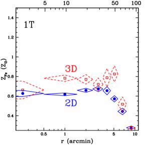
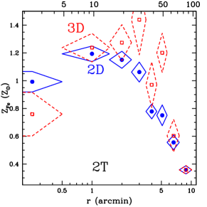
Figure 1: Radial profiles (units – bottom: arcminutes, top: kpc) of the Fe abundance and associated $1\sigma$ errors for (Left panel) 1T and (Right panel) 2T models fitted simultaneously to the XMM and Chandra data. Note that the Chandra data apply only to the inner three radial bins. In each case “3D” refers to results obtained from a spectral deprojection analysis of the XMM and Chandra data.

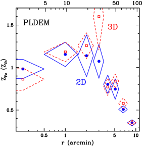
Figure 2: Same as Figure 1 except for the model with a power-law DEM (PLDEM).

Table 1: Temperatures for 1T and 2T Models

			1T (2D)	1T (3D)	2T (2D)		2T (3D)
	$R_{\rm in}$	$R_{\rm out}$	$T$	$T$	$T_{\rm c}$	$T_{\rm h}$	$T_{\rm c}$	$T_{\rm h}$
Bin	(arcmin)	(arcmin)	(keV)	(keV)	(keV)	(keV)	(keV)	(keV)
1	0.	0.5	$0.754\pm 0.005$	$0.698\pm 0.013$	$0.74\pm 0.01$	$1.66\pm 0.09$	$0.69\pm 0.01$	$3.7(>1.4)$
2	0.5	1.5	$0.807\pm 0.002$	$0.788\pm 0.003$	$0.787\pm 0.003$	$1.47\pm 0.04$	$0.772\pm 0.004$	$1.62\pm 0.07$
3	1.5	2.5	$0.985\pm 0.003$	$0.904\pm 0.006$	$0.83\pm 0.01$	$1.35\pm 0.02$	$0.82\pm 0.01$	$1.36\pm 0.06$
4	2.5	3.5	$1.172\pm 0.005$	$1.111\pm 0.018$	$0.87\pm 0.01$	$1.36\pm 0.02$	$0.86\pm 0.01$	$1.37\pm 0.06$
5	3.5	4.5	$1.236\pm 0.010$	$1.251\pm 0.019$	$0.92\pm 0.01$	$1.31\pm 0.02$	$1.05\pm 0.08$	$1.47\pm 0.13$
6	4.5	5.7	$1.229\pm 0.007$	$1.244\pm 0.017$	$0.85\pm 0.10$	$1.35\pm 0.03$	$0.86\pm 0.14$	$1.37\pm 0.04$
7	5.7	7.6	$1.205\pm 0.011$	$1.268\pm 0.025$	$0.79\pm 0.14$	$1.29\pm 0.05$	$0.50\pm 0.23$	$1.28\pm 0.05$
8	7.6	10.1	$1.147\pm 0.013$	$1.147\pm 0.015$	$0.90\pm 0.07$	$1.30\pm 0.04$	$0.90\pm 0.10$	$1.30\pm 0.05$

2.1 Preliminaries

To obtain the three-dimensional properties of the X-ray emitting gas we perform a spectral deprojection analysis assuming spherical symmetry using the (non-parametric) “onion-peeling” technique as discussed in Paper 1. We refer to deprojected models as “3D” while traditional model fits to the data on the sky are referred to as “2D” (i.e., without deprojection). However, with respect to 2D models, deprojection always inflates the errors between points which is related to the error associated with the derivative of the emissivity in an Abel inversion. As discussed in Paper 1, we perform a regularization procedure on the oxygen and neon abundances to limit their radial fluctuations in 3D models. No regularization is applied to any 2D model. Because the abundances obtained from 2D models have smaller statistical errors and do not require any regularization we shall generally present results for both 2D and 3D models in this paper. Statistical errors on the parameters are computed using the Monte Carlo procedure discussed in §4.1 of Paper 1.

We measure the Fe abundance as a function of radius using a suite of different models for the temperature distribution as described in Paper 1. Single-temperature (1T) and two-temperature (2T) models are used as our baseline models for comparison to previous studies. We also examined a set of models that emit over a continuous range of temperatures; i.e., models having a continuous differential emission measure (DEM): cooling flow, gaussian DEM, and power-law DEM (PLDEM). In every model the following abundances are free parameters: Fe, O, Ne, Mg, Si, and S – the abundances for all other elements are tied to Fe in their solar ratios. Unless stated otherwise, for every multitemperature model (e.g., 2T) the abundances of one temperature component are tied to those in the other temperature component(s). Even though the 2T and PLDEM models provide superior fits within the central $\sim 30$ kpc of NGC 5044, in this paper we present results for all models for the purpose of showing the dependence of the inferred Fe abundance on the temperature structure of the hot gas.

The reference solar Fe abundance has been a source of much confusion in the literature. There is now good agreement between values of the Fe abundance obtained from measurements in the solar photosphere and from solar-system meteorites (e.g., McWilliam, 1997; Grevesse & Sauval, 1998). Therefore, we take the solar abundances in xspec (v11.2.0af) to be those given by the Grevesse & Sauval (1998) table which use the correct Fe value, $\rm Fe/H=3.2\times 10^{-5}$ by number. Unfortunately, most previous and many current X-ray studies of Fe abundances use the incorrect “old photospheric” value of $\rm Fe/H=4.7\times 10^{-5}$ present in the Anders & Grevesse (1989) table in xspec which is still the default option in xspec. Consequently, investigators who use the old photospheric value for Fe/H obtain values for the Fe abundance that are approximately a factor 1.4 too small. In comparing with our results, we shall transform all abundances from previous studies to those of Grevesse & Sauval (1998) unless stated otherwise.

2.2 Results

The Fe abundance ($Z_{\rm Fe}$) as a function of radius obtained from 1T models fitted simultaneously to the XMM and Chandra data is displayed in Figure 1 (Left panel); note that the Chandra data only apply to the inner three radial bins. In Table 1, for convenience, we reproduce the temperature results for the 1T and 2T models from Paper 1. For $r\lesssim 50$ kpc the iron abundance is approximately constant such that $\hbox{{$Z_{\rm Fe}$}}\approx 0.65\hbox{{$Z_{\odot}$}}$ for the 1T (2D) model and $\hbox{{$Z_{\rm Fe}$}}\approx 0.75\hbox{{$Z_{\odot}$}}$ for the 1T (3D) model. At larger radii $Z_{\rm Fe}$ decreases with increasing radius with the lowest value occurring in the bounding annulus/shell: $\hbox{{$Z_{\rm Fe}$}}=0.28\pm 0.02\hbox{{$Z_{\odot}$}}$ for $r=73-97$ kpc. The $\sim 15\%$ larger values of $Z_{\rm Fe}$ obtained for the deprojected models near 40-50 kpc are primarily the result of the projection effect which tends to smear out a radially varying function, while for smaller radii they are primarily the result of the Fe Bias. In the latter case the deprojection removes the projected temperature components from exterior shells thus allowing the 1T model to be a better – though still not good – representation of the spectrum within a given shell at smaller radii.

Previous ASCA studies of NGC 5044 that fitted 1T models to the $\approx 0.5-10$ keV data in the central regions obtained much smaller abundances. For example, Fukazawa et al. (1996) obtained $\hbox{{$Z_{\rm Fe}$}}=0.46\pm 0.03\hbox{{$Z_{\odot}$}}$ for $R<20$ kpc, and Finoguenov & Ponman (1999) obtained $\hbox{{$Z_{\rm Fe}$}}=0.65\pm 0.07\hbox{{$Z_{\odot}$}}$ for $r=30-40$ kpc using 1T models of the ASCA data of NGC 5044. As we discussed in Buote (1999), 1T models are poor fits to the ASCA data extracted from large apertures because they contain a distribution of temperatures implied by the radial temperature gradients observed with ROSAT (David et al., 1994; Buote, 1999, 2000a). These temperature gradients suggested by ROSAT are confirmed and mapped in detail with Chandra and XMM in Paper 1.

The Fe abundances for the 2T models fitted simultaneously to the XMM and Chandra data are also displayed in Figure 1 (Right panel). For all radial bins interior to a radius of $\approx 40$ kpc, excluding the central bin, the values of $Z_{\rm Fe}$ obtained from the 2T models exceed by 40%-100% those obtained from the 1T models. This systematic increase arises from the Fe Bias, and the differences between the 1T and 2T models are highly significant; e.g., in shell #2 we obtain $\hbox{{$Z_{\rm Fe}$}}=0.78\pm 0.03\hbox{{$Z_{\odot}$}}$ for 1T (3D) $\hbox{{$Z_{\rm Fe}$}}=1.24\pm 0.10\hbox{{$Z_{\odot}$}}$ for 2T (3D), and $\hbox{{$Z_{\rm Fe}$}}=1.18\pm 0.12\hbox{{$Z_{\odot}$}}$ for PLDEM (3D) models. Recall from Paper 1 that the 2T and PLDEM models provide the best fits to the data, and the fit residuals observed for the 1T model near 1 keV are fully consistent with those produced by the Fe Bias.

In Figure 2 we show the Fe abundances obtained for the PLDEM model. It is notable that the PLDEM model, which fits the data almost as well as the 2T model, gives $Z_{\rm Fe}$ values consistent with the 2T model everywhere within the $1\sigma-2\sigma$ errors. The overall similarity of $Z_{\rm Fe}$ values for different multitemperature models (including cooling flow and Gaussian DEM – not shown) indicates that the value of $Z_{\rm Fe}$ can be fairly reliably inferred with any of the multitemperature models; i.e., it is principally the 1T model that suffers from the Fe Bias and gives large underestimates of $Z_{\rm Fe}$.

Focusing on the multitemperature models since they provide the best spectral fits in the central regions, we conclude that the iron abundance displays a strong gradient in NGC 5044. At the largest radius examined ($R=97$ kpc) we have $\hbox{{$Z_{\rm Fe}$}}\approx 0.35\hbox{{$Z_{\odot}$}}$. The (deprojected) iron abundance increases to values between 1-1.5 solar within $r\approx 50$ kpc for all multitemperature models and then dips within the central bin to a value of $\approx 0.8\hbox{{$Z_{\odot}$}}$.

For every model we have discussed so far (except the 1T (2D) model) the iron abundance dips in the central bin. In §8 we discuss a multi-temperature model that does not dip in the center and the implications of such a dip for enrichment models of the hot gas.

3 Silicon Abundance

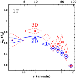
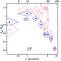
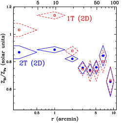
Figure 3: Radial profiles (units – bottom: arcminutes, top: kpc) of the Si abundance and associated $1\sigma$ errors for (Left panel) 1T and (Middle panel) 2T models. In each case “3D” refers to results obtained from a spectral deprojection analysis. (Right panel) $Z_{\rm Si}$/$Z_{\rm Fe}$ ratios for the 1T (2D) and 2T (2D) models.

Next to the broad feature of Fe L lines near 1 keV, the most notable emission lines in the EPIC spectra of NGC 5044 (see Paper 1) are the K$\alpha$ lines of silicon; i.e., Si XIII He$\alpha$ (1.85 keV), Si XIV Ly$\alpha$ (2.0 keV). It follows that the silicon abundance ($Z_{\rm Si}$) is also best constrained next to $Z_{\rm Fe}$. Although it might be expected that $Z_{\rm Si}$ does not suffer the same model-dependences as $Z_{\rm Fe}$ because the silicon lines are fairly isolated and well-separated from the Fe L lines, the results of the spectral fits show otherwise.

In Figure 3 we display $Z_{\rm Si}$ as a function of radius for 1T and 2T models. Analogously to $Z_{\rm Fe}$ we find that $Z_{\rm Si}$ obtained from deprojected fits (i.e., 3D) of both 1T and 2T models are systematically larger than those obtained from 2D fits by 10%-20%. For 1T models, $\hbox{{$Z_{\rm Si}$}}\approx 0.7\hbox{{$Z_{\odot}$}}$ for $r\lesssim 30$ kpc and falls to $\hbox{{$Z_{\rm Si}$}}\approx 0.2\hbox{{$Z_{\odot}$}}$ in the outermost radial bin. Similar values are obtained at large radius for 2T models. But for $r\lesssim 30$ kpc, 2T (3D) model yields $\hbox{{$Z_{\rm Si}$}}\approx 1.1\hbox{{$Z_{\odot}$}}$ for $r\lesssim 30$ kpc which dips to $\hbox{{$Z_{\rm Si}$}}\approx 0.7\hbox{{$Z_{\odot}$}}$ in the central bin in good agreement with the behavior observed for $Z_{\rm Fe}$.

The other multitemperature models (cooling flow, Gaussian DEM, power law DEM) give values for $Z_{\rm Si}$ relative to the 1T and 2T models that are entirely analogous to that described for $Z_{\rm Fe}$ in the previous section; i.e., they mostly give values consistent with the 2T model within the 1-2 $\sigma$ errors. Given that the 2T and PLDEM models provide the best fits within $r\lesssim 30$ kpc (Paper 1), and they yield fully consistent values for $Z_{\rm Fe}$ and $Z_{\rm Si}$, the near-solar values obtained for each element should be considered the favored values.

Although the silicon abundance obtained from 1T models within the central regions is biased low because of multiple temperature components having values near 1 keV within each radial bin (i.e., “Silicon Bias”, Buote, 2000b), the ratio of silicon-to-fe ($Z_{\rm Si}$/$Z_{\rm Fe}$) is affected much less. In Figure 3 (Right panel) we plot $Z_{\rm Si}$/$Z_{\rm Fe}$ as function of radius for 1T (2D) and 2T (2D) models; the 3D models are everywhere consistent with their 2D counterparts within the $1\sigma-2\sigma$ errors. The Gaussian-weighted mean of all radial bins is $\hbox{{$Z_{\rm Si}$}}/\hbox{{$Z_{\rm Fe}$}}=0.96\pm 0.02$ (in solar units) for 1T (2D) and $\hbox{{$Z_{\rm Si}$}}/\hbox{{$Z_{\rm Fe}$}}=0.83\pm 0.01$ (in solar units) for 2T (2D); the gas-mass-weighted values are $\hbox{{$Z_{\rm Si}$}}/\hbox{{$Z_{\rm Fe}$}}=0.74\pm 0.05$ and $\hbox{{$Z_{\rm Si}$}}/\hbox{{$Z_{\rm Fe}$}}=0.74\pm 0.05$ respectively for the 1T and 2T models. As expected, the largest differences between 1T and 2T models are observed within the central four bins (i.e., $r\lesssim 30$ kpc) where $\hbox{{$Z_{\rm Si}$}}/\hbox{{$Z_{\rm Fe}$}}=1.00\pm 0.02$ and $\hbox{{$Z_{\rm Si}$}}/\hbox{{$Z_{\rm Fe}$}}=0.85\pm 0.01$ respectively for the 1T and 2T models for Gaussian means and $\hbox{{$Z_{\rm Si}$}}/\hbox{{$Z_{\rm Fe}$}}=0.86\pm 0.03$ and $\hbox{{$Z_{\rm Si}$}}/\hbox{{$Z_{\rm Fe}$}}=0.80\pm 0.02$ respectively for corresponding mass-weighted means; for comparison, in the outer bins (5-8) we have $\hbox{{$Z_{\rm Si}$}}/\hbox{{$Z_{\rm Fe}$}}=0.74\pm 0.04$ (1T) and $\hbox{{$Z_{\rm Si}$}}/\hbox{{$Z_{\rm Fe}$}}=0.76\pm 0.03$ (2T) for Gaussian means and $\hbox{{$Z_{\rm Si}$}}/\hbox{{$Z_{\rm Fe}$}}=0.72\pm 0.06$ (1T) and $\hbox{{$Z_{\rm Si}$}}/\hbox{{$Z_{\rm Fe}$}}=0.73\pm 0.06$ (2T) for mass-weighted means.

We note that the marginal evidence that $\hbox{{$Z_{\rm Si}$}}/\hbox{{$Z_{\rm Fe}$}}$ decreases with radius in NGC 5044 (i.e., for the 2T model the Gaussian mean value of $\hbox{{$Z_{\rm Si}$}}/\hbox{{$Z_{\rm Fe}$}}$ for bins 5-8 is lower than that obtained from bins 1-4 by $1.9\sigma$) should be considered quite tentative because this relatively small difference could be an artifact of the simple spectral models used. (However, all models we have investigated give similar results.) If real, the slightly larger $\alpha$/Fe abundance ratios near the center might be the result of stellar mass loss which would be expected to have a lower SNe Ia fraction.

4 Other Abundances

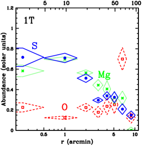
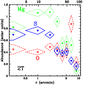
Figure 4: Radial profiles (units – bottom: arcminutes, top: kpc) of the O, Mg, and Si abundances and their associated $1\sigma$ errors for the (Left panel) 1T (2D) and (Right panel) 2T (2D) models.

In Figure 4 we show the radial abundance profiles for O, Mg, and S for the 1T (2D) and 2T (2D) models; the deprojected values (not shown) are considerably noisier and are in most cases consistent with the 2D values within the $1\sigma$ errors. Although there is considerable scatter between radii, like Si the values of the O and Mg abundances obtained with the 2T model are systematically larger than those obtained with the 1T model within $r\sim 50$ kpc. The values of S are generally consistent between the 1T and 2T models. The relative insensitivity of S to the temperature model is likely attributed to the fact that the key S emission lines near 2.4 keV are farther away from the $\sim 1$ keV Fe L lines than either O, Mg, or Si.

Although the value of the Mg abundances differs significantly between 1T and 2T models, the Mg/Fe ratio – like the Si/Fe ratio – is quite similar for both models; e.g., in bin #2, $\hbox{{$Z_{\rm Mg}$}}/\hbox{{$Z_{\rm Fe}$}}=0.94\pm 0.05$ in solar units, for 1T (3D) while, $\hbox{{$Z_{\rm Mg}$}}/\hbox{{$Z_{\rm Fe}$}}=0.88\pm 0.05$ in solar units, for 2T (3D). But the O/Fe and S/Fe ratios do show significant differences between the models, although the O/Fe ratio is very sub-solar in both cases; e.g., in bin #2, $\hbox{{$Z_{\rm O}$}}/\hbox{{$Z_{\rm Fe}$}}=0.19\pm 0.04$ and $\hbox{{$Z_{\rm S}$}}/\hbox{{$Z_{\rm Fe}$}}=0.96\pm 0.08$ in solar units, for 1T (3D) while, $\hbox{{$Z_{\rm O}$}}/\hbox{{$Z_{\rm Fe}$}}=0.30\pm 0.05$ and $\hbox{{$Z_{\rm S}$}}/\hbox{{$Z_{\rm Fe}$}}=0.66\pm 0.05$ in solar units, for 2T (3D). We note that the oxygen abundance in bin #7 is significantly larger ($\approx 4\sigma$) than its values in adjacent bins. We do not believe the fluctuation in the oxygen abundance in bin #7 is physical, but we have not yet isolated the cause.

For the 2T (3D) model we obtain Gaussian weighted mean values of all radial bins of $\hbox{{$Z_{\rm S}$}}/\hbox{{$Z_{\rm Fe}$}}=0.62\pm 0.04$, $\hbox{{$Z_{\rm O}$}}/\hbox{{$Z_{\rm Fe}$}}=0.39\pm 0.03$, and $\hbox{{$Z_{\rm Mg}$}}/\hbox{{$Z_{\rm Fe}$}}=0.88\pm 0.04$ in solar units; the corresponding gas-mass-weighted means are $\hbox{{$Z_{\rm S}$}}/\hbox{{$Z_{\rm Fe}$}}=0.46\pm 0.10$, $\hbox{{$Z_{\rm O}$}}/\hbox{{$Z_{\rm Fe}$}}=0.56\pm 0.09$, and $\hbox{{$Z_{\rm Mg}$}}/\hbox{{$Z_{\rm Fe}$}}=0.66\pm 0.17$ in solar units. Ignoring the anomalous bin #7 we obtain $\hbox{{$Z_{\rm O}$}}/\hbox{{$Z_{\rm Fe}$}}=0.37\pm 0.03$ (Gaussian averaged) and $\hbox{{$Z_{\rm O}$}}/\hbox{{$Z_{\rm Fe}$}}=0.37\pm 0.04$ (mass averaged) including only bins 1-6.

Finally, we mention that the Ne abundance (not shown) is the most poorly constrained abundance that we have investigated. Undoubtedly the poor constraints are at least partially attributed to the location of the strongest Ne lines near 1 keV which are therefore completely blended with the Fe L lines in the CCD spectra. Generally, we find very sub-solar values for the Ne abundance except within $r\sim 10$ kpc where near solar values are suggested. More precise constraints are provided for the emission-weighted average Ne abundance in §7.

5 Non-Azimuthally Symmetric Analysis

Following our discussion in §5 of Paper 1 we searched for azimuthal variations in the iron abundance by fitting 1T and 2T models to spectra extracted from circular apertures arranged in a square array on the EPIC MOS images. Consistent with the results for the temperatures discussed in Paper 1, we find that overall the abundances obtained from this analysis are consistent with the spherically symmetric analysis. In particular, we find no evidence for azimuthal abundance variations associated with the small azimuthal temperature variations between radii of $2\arcmin-3\arcmin$ mentioned in Paper 1. We also observe the same increase in the iron abundance for apertures within $r\sim 30$ kpc for 2T over 1T models that is obtained in the spherically symmetric (i.e., azimuthally averaged) analysis.

6 Systematic Errors

This section contains a detailed investigation of systematic errors on the abundance measurements. Those readers who are not interested in these technical details can safely skip ahead to §7.

6.1 Calibration

Table 2: Comparison of Fe Abundances from Chandra and XMM

	1T			2T
	XMM	Chandra	%	XMM		Chandra		%	%
Annulus	(free)	(free)	(free)	(free)	(fix)	(free)	(fix)	(free)	(fix)
1	$0.64\pm 0.05$	$0.61\pm 0.05$	$5\pm 1$	$1.17\pm 0.13$	$1.04\pm 0.13$	$0.83\pm 0.09$	$0.90\pm 0.09$	$29\pm 14$	$13\pm 16$
2	$0.58\pm 0.02$	$0.68\pm 0.03$	$-17\pm 6$	$1.27\pm 0.07$	$1.20\pm 0.07$	$1.11\pm 0.07$	$1.20\pm 0.07$	$13\pm 8$	$0\pm 8$
3	$0.65\pm 0.03$	$0.67\pm 0.03$	$-3\pm 6$	$1.30\pm 0.07$	$1.24\pm 0.07$	$0.99\pm 0.08$	$1.13\pm 0.08$	$24\pm 9$	$9\pm 9$

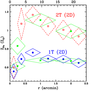
Figure 5: Radial profiles (units – bottom: arcminutes, top: kpc) of the Fe abundance and associated $1\sigma$ errors for 1T (blue circles and solid diamonds) and 2T (red boxes and dashed diamonds) models. Only the Chandra data are used and each model is 2D; i.e., not obtained from the spectral deprojection analysis. We also show for each model (green crosses and dashed diamonds) the results obtained in the wider apertures used in the joint XMM and Chandra fits; the results for these fits are given in Table 2.

We have examined possible systematic errors in the measurements of the metal abundances arising from calibration differences between the XMM MOS, XMM pn, and Chandra ACIS-S3 CCDs. In Table 2 we list the values of $Z_{\rm Fe}$ obtained from 1T (2D) and 2T (2D) models fitted separately to the XMM and Chandra data; i.e., the MOS and pn data were fitted simultaneously while the Chandra data were fitted alone. We focus on 2D models so that the fits for a specific annulus are independent of results obtained from fits to adjacent regions at larger radii.

Using the 1T model the XMM and Chandra data in annuli 1 and 3 give values of $Z_{\rm Fe}$ that agree within 5%. In annulus 2 the value obtained from XMM is $17\%\pm 6\%$ lower than that obtained from Chandra. The significance of this discrepancy is not very high. However, it is noteworthy that in annulus 2 we find the largest improvement for a 2T model over a 1T model (Paper 1). Given the very poor fit of the 1T (2D) model within annulus 2 the modest discrepancy of $17\%\pm 6\%$ between detectors could simply arise from the different energy-dependent sensitivities of the detectors.

The effects of different sensitivities are illustrated by the 2T (2D) fits also listed in Table 2. If the relative normalizations of the two temperature components are allowed to be different for XMM and Chandra (i.e., denoted by “free” in Table 2), then we find that the values of $Z_{\rm Fe}$ obtained from XMM exceed those obtained by Chandra by 15%-30%. However, if we fix the relative normalizations of the cooler and hotter components to their best-fitting values obtained from the joint XMM-Chandra fits (i.e., denoted by “fix” in Table 2), then we find no significant differences between the XMM and Chandra fits; i.e., the percentage differences are all less than the (relatively large) $1\sigma$ errors. Since the difference of the quality of the fits (not shown) is quite negligible between the fixed and free cases, the different values of $Z_{\rm Fe}$ obtained in the two cases are probably attributed to the different energy-dependent sensitivities of the XMM and Chandra detectors. We conclude that errors in the relative calibration between XMM and Chandra contribute errors in the measured value of $Z_{\rm Fe}$ of less than 20%.

The agreement of $Z_{\rm Fe}$ obtained from the Chandra and XMM CCDs also indicates that the larger PSF of XMM does not significantly affect our results; i.e., we have chosen bins that are sufficiently wide for the XMM PSF – consistent with our findings regarding the temperature profile in Paper 1.

(We mention that we have performed an identical study to assess differences in $Z_{\rm Fe}$ measured between the XMM MOS and pn CCDs. For annuli 5-8 we find that the values of $Z_{\rm Fe}$ obtained from separate fitting of the MOS and pn data generally agree within their 1-2 $\sigma$ errors. However, for annuli 1-4 the values of $Z_{\rm Fe}$ obtained from the pn data always exceed the values obtained from the MOS by as little as 10% to as much as 50%, with the MOS values usually agreeing better with the Chandra data in their regions of overlap. As a result, we explored using only the MOS and Chandra data in our analysis but found that the errors in the deprojected $Z_{\rm Fe}$ abundances were sufficiently large that we had to regularize the iron abundance to obtain a radial profile similar to the 2D result. After this regularization we noticed that the results were quite consistent with the original un-regularized $Z_{\rm Fe}$ values obtained from the simultaneous MOS+pn fits. Because of this agreement, and the fact that the MOS+pn fits do not require $Z_{\rm Fe}$ to be regularized, the good agreement of the MOS+pn fits with the Chandra fits discussed above, and the excellent agreement of the MOS+pn and ASCA data discussed in §7, we decided to use all of the data sets in our default analysis.)

As in Paper 1 we also performed fits to the Chandra data within annuli that are half the size of those used for the XMM and joint XMM – Chandra fits. In Figure 5 we show $Z_{\rm Fe}$ obtained from 1T (2D) and 2T (2D) fits to the Chandra data in annuli of $30\arcsec$ width between $0.5\arcmin-2.5\arcmin$ and $15\arcsec$ width between $0\arcsec-30\arcsec$ (see also Table 5 and Figure 6 in Paper 1). Also shown in Figure 5 are the results using the larger $1\arcmin$-width annuli for the results obtained from the joint XMM – Chandra fits. The values for $Z_{\rm Fe}$ obtained in the larger bins are mostly consistent with an average value of $Z_{\rm Fe}$ obtained in the thinner bins. Moreover, if the hot gas is actually single-phase, we would have expected in the smaller bins to have a smaller radial temperature variation, and thus a weaker “Fe Bias”, and therefore a smaller underestimate of $Z_{\rm Fe}$ using the 1T model. Instead, we see good agreement between the $Z_{\rm Fe}$ values obtained using the thinner and wider bins. (Note: consistent results are obtained with 3D models using the XMM data to deproject shells exterior to $r=2.5\arcmin$.) This agreement is consistent with the models for limited multiphase gas (i.e., particularly the 2T and PLDEM models.)

In Figure 5 one also notices that the central dip in $Z_{\rm Fe}$ is apparently a smooth transition beginning within the Chandra annulus $R=15\arcsec-30\arcsec$ and finishing within the central bin. It is within the central bin ($R=15\arcsec$) where the value of $Z_{\rm Fe}$ obtained from the 1T and 2T models (2D) agree best.

As discussed in §6.1.2 of Paper 1 the value of $Z_{\rm Fe}$ obtained from the XMM RGS data of NGC 5044 by Tamura et al. (2003) is in excellent agreement with the value we obtain from the simultaneous fits to the XMM and Chandra CCDs in the central radial bin. We emphasize that this excellent agreement occurs when the same models (with the same free parameters) are fitted over the same energy range for both the RGS and the CCDs. The good agreement provides a further check on possible calibration differences between detectors.

We conclude that both the XMM and Chandra CCD data require $Z_{\rm Fe}$ to be at least solar within $r\sim 30$ kpc except for within the very central region ($r=2.4$ kpc).

6.2 Plasma Codes

Figure 6: Comparison of the apec and mekal plasma codes in the energy region, 0.7-1.2 keV, where the Fe L shell emission lines dominate for a $\sim 1$ keV plasma. We show the apec/mekal ratio for a $T=1$ keV, solar metallicity plasma (Left panel) at high resolution and (Right panel) at moderate resolution, the latter corresponding approximately to the response matrix binning of the MOS data of NGC 5044 we used in our spectral fitting.

For a single isolated emission line of a particular element in a coronal plasma the abundance of that element may be directly measured by calculating the ratio of the flux within the line to the flux of the local continuum. In such an idealized case, any error in the theoretical calculation of the line flux within the plasma code will translate directly to an error in the measured elemental abundance. Consider, however, the case of the Fe L shell lines for a system like NGC 5044.

In a coronal plasma with $T\sim 1$ keV there is a forest of Fe L lines near $1$ keV, with the most important lines spanning the approximate range 0.7-1.2 keV. Consider also these lines when observed at the moderate spectral resolution of the XMM and Chandra CCDs ($\Delta E\approx 50-100$ eV near 1 keV). In these cases the Fe abundance is obtained by fitting data over a broad energy range, so that all of the strong Fe L lines over 0.7-1.2 keV play a key role as does the continuum determined from regions outside the Fe L region. The net effect is that even rather large errors in a small number of lines do not necessarily translate directly to large errors in the inferred Fe abundance.

We illustrate this effect in Figure 6 using the apec and mekal plasma codes. These codes have many differences in how they model the atomic physics and in their line libraries (especially for Fe L) thus allowing for an interesting test of the robustness of the iron abundance determination. We consider a fiducial spectral model with $T=1$ keV, $Z=1\hbox{{$Z_{\odot}$}}$, and equal normalizations for the apec and mekal codes. The ratio of the fluxes in the two models are plotted as a function of energy over the range 0.7-1.2 keV for two different resolutions. In the left panel we plot this ratio at high-resolution binning ($\Delta E=0.5$ eV) giving 1000 energy bins over the energy range shown. Although most of the points cluster near 1, there are many points having large errors; i.e., ratios larger than 2 or less than 1/2. In the right panel we plot the same ratio at the binning for the moderate resolution CCDs ($\Delta E=15$ eV) used in our analysis of NGC 5044; specifically, these energy bin sizes correspond to those of the re-binned MOS1 data in the central radial bin for NGC 5044. In this case the ratios are all within $\approx 20\%$, and thus we should expect that the iron abundances should not differ by much more than this amount for each model.

Indeed, we find that both 1T and 2T models (each 2D) computed using the apec code differ by no more than 10%-20% from those computed using the mekal code. Interestingly, the small differences between apec and mekal do appear to be a real systematic effect despite the fact that these differences are consistent within the $1\sigma$ errors. The sign of the systematic difference is opposite for 1T and 2T models: for 1T models, $\hbox{{$Z_{\rm Fe}$}}^{\rm apec}>\hbox{{$Z_{\rm Fe}$}}^{\rm mekal}$, while for 2T models, $\hbox{{$Z_{\rm Fe}$}}^{\rm apec}<\hbox{{$Z_{\rm Fe}$}}^{\rm mekal}$.

We conclude that the measured iron abundances are accurate to within 10%-20% considering reasonable remaining errors in the plasma codes such as those associated with the Fe XVII lines near 0.7 keV discussed by Behar et al. (2001). Of course, for high-resolution studies using the gratings on Chandra and XMM more care must be taken when analyzing the properties of individual lines such as done by Behar et al. (2001). But even high-resolution studies of NGC 5044 using the RGS obtain fully consistent values for $Z_{\rm Fe}$ from broad-band spectral fitting with the values obtained from the XMM and Chandra CCDs as discussed at the end of §6.1.

6.3 Bandwidth

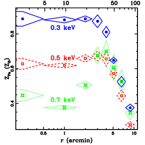
Figure 7: Radial profiles (units – bottom: arcminutes, top: kpc) of the Fe abundance and associated $1\sigma$ errors for the 1T (2D) model obtained from fitting data with lower energy limit $\hbox{{$E_{\rm min}$}}=0.3,0.5,0.7$ keV.

In section 5.1 of Buote (2000a) we discussed the sensitivity of the Fe Bias to the lower energy limit used in the spectral fitting of a $T\sim 1$ keV coronal plasma. Here we summarize this discussion and refer the interested reader to the previous paper for details. Consider (1) a 1T model ($T=1$ keV) of a coronal plasma with solar metallicity, and (2) a multitemperature coronal model with temperature components distributed across $T\approx 0.7-1.5$ keV also with solar metallicity; e.g., the simplest case of a 2T model with $\hbox{{$T_{\rm c}$}}=0.7$ keV and $\hbox{{$T_{\rm h}$}}=1.5$ keV each with the same emission measure. Each model has the same total emission measure. The spectral energy distribution of the 1T model has a much narrower peak near 1 keV than the 2T model; see Figure 5 of Buote (2000a).

If the observed spectrum is similar to the 2T model, such as we observe for NGC 5044 with XMM and Chandra within $r\sim 30$ kpc, then the 1T model with solar metallicity is a poor fit to the data. If the iron abundance is allowed to vary, then the fitting software (xspec in this case) tries to improve $\chi^{2}$ near 1 keV by reducing the value of $Z_{\rm Fe}$ while simultaneously raising the continuum to maintain the quality of the fit near the wings of the Fe L region. The resulting Fe abundance obtained with the 1T model is therefore an underestimate of the true value. It is this effect that we have previously termed the “Fe Bias” (e.g., Buote, 2000b, a).

However, the ability of the $\chi^{2}$ fitter to increase the contribution of the continuum within the Fe L region depends sensitively on the constraints on the continuum outside the Fe L region. At higher energies the model compensates for this increase in the continuum by simultaneously decreasing the abundances of Mg, Si, and S while maintaining an approximately fixed $\alpha$/Fe ratio as discussed in §3 and 4; note that Mg, Si, and S have the strongest emission lines at energies above the Fe L region in NGC 5044.

At energies below the Fe L region (i.e., below 0.7 keV), the strongest line is far and away O VIII ly-$\alpha$ near 0.65 keV – very close to the bottom edge of the Fe L region. Below the O VIII line down to the $\sim 0.3$ keV bandpass limits of the XMM and Chandra CCDs there are no strong emission lines. (Allowing the C and N abundances to vary affects the inferred value of $Z_{\rm Fe}$ by $<10\%$.) Therefore, possible changes in the continuum level below the O VIII ly-$\alpha$ line requested by the $\chi^{2}$ fitter to better match the Fe L region cannot be compensated for by changes in the elemental abundances. Changing the temperature is also not an option since it is tightly constrained by the shape of the continuum both above and below the Fe L region. (It is found that the inferred temperature of the 1T model is quite insensitive to the fitted – or assumed – value of $Z_{\rm Fe}$ over a large range in $Z_{\rm Fe}$.) Hence, below $\approx 0.7$ keV the continuum data are a strong inhibitor of the Fe Bias, though they do not prevent it entirely as demonstrated by the differences we obtained for 1T and multitemperature models discussed in §2.

Consequently, it is expected that for spectra where the Fe Bias is unimportant (e.g., the XMM spectra for $r\gtrsim 40$ kpc in NGC 5044) the measured value of $Z_{\rm Fe}$ should not be very sensitive to the value of $E_{\rm min}$ – the lower energy limit (0.3-0.7 keV) used in the spectral fitting. In contrast, for spectra where the Fe Bias is important (e.g., the XMM spectra for $r\lesssim 30$ kpc in NGC 5044) the measured value of $Z_{\rm Fe}$ should be very sensitive to the value of $E_{\rm min}$, and specifically $Z_{\rm Fe}$ should decrease as $E_{\rm min}$ increases toward 0.7 keV.

This behavior is observed for NGC 5044. In Figure 7 we plot $\hbox{{$Z_{\rm Fe}$}}(R)$ for the 1T (2D) model fitted jointly to the Chandra and XMM data for different values of $\hbox{{$E_{\rm min}$}}=0.3,0.5,0.7$ keV. For $R\gtrsim 40$ kpc the values of $Z_{\rm Fe}$ for $\hbox{{$E_{\rm min}$}}=0.3,0.7$ keV agree within their $\sim 1\sigma$ errors. The values for $\hbox{{$E_{\rm min}$}}=0.5$ keV are somewhat below these values because of the degeneracy with the oxygen abundance. (If the oxygen abundance is tied to the iron abundance in their solar ratio then the $Z_{\rm Fe}$ values for $\hbox{{$E_{\rm min}$}}=0.5$ keV are within 10%-20% of the values of the other $E_{\rm min}$.) For $R\lesssim 30$ kpc, where we have the evidence for multitemperature gas and the corresponding Fe Bias, we observe that $Z_{\rm Fe}$ decreases as $E_{\rm min}$ increases toward 0.7 keV as expected.

We mention that the $Z_{\rm Fe}$ values inferred from 2T models also follow the same trends, though not as dramatically as for the 1T models within $R\lesssim 30$ kpc. The reason why 2T models are affected at all is that the need for multitemperature models decreases (though is not removed) as $E_{\rm min}$ approaches 0.7 keV as discussed in Section 4.4 of Paper 1. Since a single temperature component dominates more in the fits for larger $E_{\rm min}$, the multitemperature models suffer more from the Fe Bias for larger $E_{\rm min}$. For example, the best-fitting values of $Z_{\rm Fe}$ for the 2T (2D) model in radial bin #2 are respectively $(1.38,1.19,0.86)$ in solar units for $\hbox{{$E_{\rm min}$}}=0.3,0.5,0.7$ keV. These values still exceed their respective purely 1T (2D) counterparts by a factor of $\approx 2$.

Hence, for $T\sim 1$ keV plasmas consisting of multiple temperature components distributed across $T\approx 0.7-1.5$ keV, we conclude that reliable measurements of $Z_{\rm Fe}$ can only be obtained for $E_{\rm min}$ below $\approx 0.5$ keV since the continuum emission below 0.6 keV serves as an important check on the Fe Bias. In this paper we have decided to emphasize results obtained for $\hbox{{$E_{\rm min}$}}=0.5$ keV rather than for $\hbox{{$E_{\rm min}$}}=0.3$ keV because of the somewhat better agreement obtained for the values of $Z_{\rm Fe}$ between the XMM and Chandra detectors for $\hbox{{$E_{\rm min}$}}=0.5$ keV discussed in §6.1. However, the 10%-20% larger values of $Z_{\rm Fe}$ obtained from the joint XMM-Chandra fits for $\hbox{{$E_{\rm min}$}}=0.3$ keV should be considered a reasonable estimate of the systematic error arising from the choice of $E_{\rm min}$ for the results quoted in this paper.

6.4 Variable $N_{\rm H}$ and Intrinsic Absorption

Allowing for absorption by cold gas ($T\lesssim 10^{4}$ K) with a hydrogen column density ($N_{\rm H}$) in excess of the Galactic value ($\hbox{{$N_{\rm H}^{\rm Gal}$}}=5\times 10^{20}$ cm^-2) affects the values of $Z_{\rm Fe}$ obtained from single-temperature models in much the same way as increasing $E_{\rm min}$ toward 0.7 keV with $\hbox{{$N_{\rm H}$}}=\hbox{{$N_{\rm H}^{\rm Gal}$}}$ as discussed above in §6.3. That is, the values of $Z_{\rm Fe}$ obtained from 1T fits with $\hbox{{$E_{\rm min}$}}=0.7$ keV and $\hbox{{$N_{\rm H}$}}=\hbox{{$N_{\rm H}^{\rm Gal}$}}$ are broadly similar to those obtained from 1T fits with $N_{\rm H}$ in excess of $N_{\rm H}^{\rm Gal}$ for $\hbox{{$E_{\rm min}$}}=0.3-0.7$ keV; our fiducial absorber model is a foreground screen ($A(E)=\exp(-\hbox{{$N_{\rm H}$}}\sigma(E))$) with separate values of $N_{\rm H}$ for each annulus, although we have explored a suite of absorber models (e.g., with redshift at NGC 5044) and have obtained fully consistent results.

As discussed in §6.4 of Paper 1 the 2T model is still clearly preferred over the 1T model when allowing for variable $N_{\rm H}$ in each case. Unlike for the 1T models, the values of $Z_{\rm Fe}$ obtained for the multitemperature models with variable $N_{\rm H}$ only differ significantly with the corresponding model with Galactic $N_{\rm H}$ in shell #2; e.g., for the 2T (2D) model we have, $\hbox{{$Z_{\rm Fe}$}}=0.96\pm 0.05\hbox{{$Z_{\odot}$}}$ (variable $N_{\rm H}$) and $\hbox{{$Z_{\rm Fe}$}}=1.19\pm 0.06\hbox{{$Z_{\odot}$}}$ (Galactic $N_{\rm H}$) – though in both cases $Z_{\rm Fe}$ is near the solar value. Since (as discussed in Paper 1) the multitemperature models with $\hbox{{$N_{\rm H}$}}=\hbox{{$N_{\rm H}^{\rm Gal}$}}$ provide better fits than 1T models with variable $N_{\rm H}$ within the central $\approx 30$ kpc, there is no obvious sharp absorption feature in the spectrum, and there is no evidence from observations in other wavebands for the large quantities of cold absorbing material ($>10^{9}\hbox{{$M_{\sun}$}}$) implied by the fitted values of $N_{\rm H}$, we do not take seriously the results obtained from the intrinsic cold absorber models.

We mention that a collisionally ionized “warm” absorber ($T\approx 10^{5-6}$ K) model, in contrast to the cold absorber, does not affect significantly energies below $\sim 0.5$ keV and results in fitted values of $Z_{\rm Fe}$ quite similar to the models without any intrinsic absorption. Another interesting feature of the warm absorber is that the fitted oxygen abundances in the hot gas in the central regions are $\approx 0.6\hbox{{$Z_{\odot}$}}$ and the Mg/O ratios are near solar. The near-solar Mg/O ratios are in much better agreement with expectations from SNe enrichment than the values obtained for all other models we explored without a warm absorber. However, like the cold absorber there is no evidence for the emission in other wavebands implied by the relatively large column densities obtained in the X-ray fits for the warm absorber, nor is it easy to understand how the temperature of the warm gas is maintained. Consequently, we do not discuss either the warm or cold intrinsic absorbers further.

6.5 Background

We considered the effect of errors in the background normalization on the measured values of $Z_{\rm Fe}$. Apart from the few emission lines from calibration sources in the XMM and Chandra CCDs, the background is a smooth and slowly varying function of energy over the 0.3-5 keV bandpass. Consequently, if the background contribution to the spectrum is underestimated, one will believe the continuum emission is larger than in reality. As a result, one will mistakenly infer smaller equivalent widths for the emission lines and therefore underestimate the values for the metal abundances. Over-subtraction of the background leads to larger equivalent widths and overestimates of the metal abundances.

To examine the sensitivity of the measured values of $Z_{\rm Fe}$ to reasonable background errors we repeated our analysis using the background templates renormalized to have count rates +20% and -20% of their nominal values. By fitting 1T (2D) and 2T (2D) models to the background-subtracted data using these renormalized templates, we calculated the variation in $Z_{\rm Fe}$ as a function of radius for each case. In the outer annuli (bins #7 and #8), where the background is most important, we find that the measured values of $Z_{\rm Fe}$ change by $<\pm 15\%$ with respect to the nominal background case. The variation is progressively smaller at smaller radii being $<\pm 1\%$ in the central bin.

We mention that even extreme errors in the background do not generate qualitatively different results in the measured values of $Z_{\rm Fe}$, especially within the central $R\sim 30$ kpc. For example, if we do not subtract the background at all the value of $Z_{\rm Fe}$ is underestimated by $<10\%$ for 1T (2D) models and overestimated by $<5\%$ for 2T (2D) models within radial bins 1-3. The reason why the 2T models here give a slight overestimated of $Z_{\rm Fe}$ when the background is under-subtracted is because the excess continuum at higher energies is interpreted as part of the higher temperature component. The increased normalization of this component causes an increase in the inferred value of $Z_{\rm Fe}$ according to the Fe Bias mechanism (e.g., see discussion at the beginning of §6.3). At the largest radius (bin 8), if the background is not subtracted at all we obtain best-fitting values: $\hbox{{$Z_{\rm Fe}$}}=0.17\hbox{{$Z_{\odot}$}}$ compared to the nominal value of $\hbox{{$Z_{\rm Fe}$}}=0.28\hbox{{$Z_{\odot}$}}$ for 1T, and $\hbox{{$Z_{\rm Fe}$}}=0.33\hbox{{$Z_{\odot}$}}$ compared to the nominal value of $\hbox{{$Z_{\rm Fe}$}}=0.36\hbox{{$Z_{\odot}$}}$ for 2T.

7 Emission-Weighted Average Abundances and The Fe Bias Revisited

7.1 Central Regions

Figure 8: MOS1, MOS2, and pn spectra accumulated within a circular aperture of radius, $R=5\arcmin$ (48 kpc), fitted with (Left panel) a single temperature (1T) model and (Right panel) a two-temperature (2T) model; both models are 2D. In each case the apec plasma model is used and the solar abundances are taken from Grevesse & Sauval (1998) which use the new (smaller) photospheric value for the iron abundance. The models are the same as discussed in §2 for the spatially resolved analysis. That is, Galactic absorption is assumed and the following metal abundances are free parameters: O, Ne, Mg, Si, S, Fe and all other abundances are tied to Fe in their solar ratios. For the 2T model the abundances of each temperature component are tied together in the fits.

Table 3: Emission-Weighted Average Abundances Within $R=5\arcmin=48$ kpc

	Best	$\Delta$Statistical	$\Delta$Model	$\Delta$Plasma Code	$\Delta$$E_{\rm min}$	$\Delta\hbox{{$N_{\rm H}$}}$	$\Delta$Background
$Z_{\rm Fe}$	1.09	$\pm 0.04$	$\pm 0.01$	$-0.05$	$+0.23$	$\pm 0.03$	$\pm 0.01$
$Z_{\rm Si}$/$Z_{\rm Fe}$	0.832	$\pm 0.017$	$\pm 0.004$	$+0.058$	$+0.013$	$\pm 0.011$	$\pm 0.003$
$Z_{\rm S}$/$Z_{\rm Fe}$	0.542	$\pm 0.020$	$\pm 0.006$	$+0.028$	$-0.021$	$\pm 0.002$	$\pm 0.002$
$Z_{\rm O}$/$Z_{\rm Fe}$	0.331	$\pm 0.028$	$\pm 0.005$	$-0.052$	$+0.089$	$\pm 0.014$	$\pm 0.003$
$Z_{\rm Mg}$/$Z_{\rm Fe}$	0.874	$\pm 0.026$	$\pm 0.013$	$+0.026$	$+0.055$	$\pm 0.023$	$\pm 0.005$
$Z_{\rm Ne}$	0.56	$\pm 0.09$	$\pm 0.10$	$-0.37$	$+0.26$	$\pm 0.04$	$\pm 0.03$

Irrespective of whether the hot gas at each radius is actually single-phase or multiphase, all models of the spatially varying spectra that we investigated in Paper 1 require that the accumulated spectra within $R\sim 30$ kpc contain a range of temperature components with $T\approx 0.7-1.2$ keV. Fitting a 1T model to this entire accumulated spectrum must fail according to the Fe Bias as summarized at the beginning of §6.3.

We demonstrate this manifestation of the Fe Bias as follows. We extracted the accumulated spectra of the XMM EPIC MOS1, MOS2, and pn data within a radius of $5\arcmin$ (48 kpc); we choose a radius slightly larger than 30 kpc to fully enclose the peak of the 1T temperature profile (Paper 1, Figure 3) and to facilitate comparison to previous ASCA results below. (Note the Chandra ACIS-S3 data do not extend to this radius.) The result of fitting a 1T apec model simultaneously to the MOS1, MOS2, and pn data is shown in Figure 8. Readily apparent are the residuals characteristic of the Fe Bias seen in the smaller apertures in Paper 1 and in the larger apertures in our previous ASCA studies of the brightest elliptical galaxies in centrally E-dominated groups (see especially Figure 5 in Buote 2000a and the Appendix in Buote 2000b). The fit is formally of very poor quality ($\chi^{2}=3354.5$ for 816 dof) and the iron abundance is $0.51\pm 0.01\hbox{{$Z_{\odot}$}}$. We reiterate that the poor fit and low value of $Z_{\rm Fe}$ are exactly as expected because of the presence of multitemperature temperature components within the aperture – but we have made no assumption about whether these components arise from a radially varying single-phase or a true multiphase medium.

A vastly improved fit which (1) eliminates the residuals near 1 keV to a magnitude similar to that present at other energies, and (2) provides a value of $Z_{\rm Fe}$ over twice as large as the 1T value is obtained using a simple 2T model (i.e., discrete temperature distribution) or a PLDEM (i.e., continuous temperature distribution). Each of these models adds only 2 free parameters over those of the 1T model. In Figure 8 we display the 2T model fitted to the total accumulated EPIC spectra within 48 kpc. It is clear that the residuals near 1 keV are greatly reduced the fit is improved dramatically ($\chi^{2}=1202.3$ for 814 dof). The temperatures obtained for the 2T model are $\hbox{{$T_{\rm c}$}}=0.804\pm 0.004$ keV and $\hbox{{$T_{\rm h}$}}=1.38\pm 0.02$ keV which are very similar to the range of values obtained from the spatially resolved 1T and 2T models (Paper 1); note that the best-fitting ratio of emission measures of the hotter and cooler components is 1.04. Moreover, the iron abundance for the 2T model is a factor of 2.1 times larger than obtained for the 1T model: $\hbox{{$Z_{\rm Fe}$}}=1.08\pm 0.04\hbox{{$Z_{\odot}$}}$ (statistical error). The PLDEM gives a fit and abundance values extremely similar to the 2T model: $\chi^{2}=1235.1$ for 814 dof and $\hbox{{$Z_{\rm Fe}$}}=1.10\pm 0.04\hbox{{$Z_{\odot}$}}$. (Note we obtain the following temperature parameters for the PLDEM: $\alpha=-1.2\pm 0.2$, $\hbox{{$T_{\rm min}$}}=0.665\pm 0.008$ keV, $\hbox{{$T_{\rm max}$}}-\hbox{{$T_{\rm min}$}}=1.12\pm 0.05$ keV.)

The superb agreement between the 2T and PLDEM models demonstrates that the EPIC spectral data accumulated within 48 kpc have both sufficient sensitivity and resolution to unequivocally rule out the 1T model (as expected) while constraining the DEM well enough so that fully consistent values for the abundances are obtained using very different multitemperature models; i.e., the average (emission-weighted) abundances within 50 kpc are very well constrained by the EPIC data.

In Table 3 we list the value of $Z_{\rm Fe}$ obtained from the multitemperature fits within 50 kpc and present a detailed accounting of the error budget following our discussion in §6. It is noteworthy that the largest source of error is $E_{\rm min}$ which leads to a larger value. The emission-weighted value of $Z_{\rm Fe}$ is a consistent average of the values within 50 kpc obtained from the spatially resolved analysis (Figure 1).

Also shown in Table 3 are the emission-weighted average abundance ratios $Z_{\rm Si}$/$Z_{\rm Fe}$, $Z_{\rm S}$/$Z_{\rm Fe}$, $Z_{\rm O}$/$Z_{\rm Fe}$, and $Z_{\rm Mg}$/$Z_{\rm Fe}$ obtained within 50 kpc and their associated error budgets. These ratios are very tightly constrained and agree with the mass-averaged values obtained from the spatially resolved analysis (§3 and 4). We mention that the $Z_{\rm Mg}$/$Z_{\rm Fe}$ ratio is well constrained, and the only source of error we believe could possibly account for its relatively large value is incomplete subtraction of the Al calibration lines near 1.4 keV. However, the small error in the abundance ratios associated with reasonable background errors make this explanation seem implausible as well.

The Ne abundance and its error budget are also shown in Table 3. Since the key Ne emission line is well hidden within the Fe L forest, the value of $Z_{\rm Ne}$ is quite susceptible to differences in the temperature model and plasma code. In fact, it exhibits by far the largest differences between the apec and mekal plasma code. Despite the relatively large systematic errors, the value of $Z_{\rm Ne}$ is clearly sub-solar with probably values between 0.3-0.5 solar.

Although we have established that calibration errors should contribute at most 20% extra uncertainty in the measured value of $Z_{\rm Fe}$ (§6.1), we can provide a further calibration check by comparing to our previous ASCA studies of NGC 5044 (Buote & Fabian, 1998; Buote, 1999). Buote & Fabian (1998) analyzed the ASCA SIS0 and SIS1 spectra accumulated within circles of $R\approx 5\arcmin$ centered on NGC 5044. They fitted mekal plasma models over 0.5-5 keV where (1) all abundances were tied to iron in their solar ratio, (2) the solar abundance table of Anders & Grevesse (1989) was used, and (3) the absorption column density was a free parameter. They obtained $\hbox{{$Z_{\rm Fe}$}}=0.25\hbox{{$Z_{\odot}$}}$ for the 1T model (no error given because of the poor fit) and $\hbox{{$Z_{\rm Fe}$}}=0.62^{+0.11}_{-0.08}\hbox{{$Z_{\odot}$}}$ (90% confidence) for the 2T model; the 2T model was a clearly superior fit (see Figures 1 and 5 of Buote & Fabian 1998). If we perform fits to the XMM EPIC data in the same region using exactly the same models we obtain $\hbox{{$Z_{\rm Fe}$}}=0.256\pm 0.003\hbox{{$Z_{\odot}$}}$ for 1T and $\hbox{{$Z_{\rm Fe}$}}=0.64\pm 0.02\hbox{{$Z_{\odot}$}}$ for 2T (only statistical error quoted) in excellent agreement with our previous results from ASCA. (Similar agreement is obtained when comparing identical models to Buote 1999.) The excellent agreement between XMM and ASCA implies that calibration error cannot be a large contributor to error in our measurement of $Z_{\rm Fe}$, certainly $<10\%$.

Hence, the XMM data of NGC 5044, whether extracted in a large 50 kpc aperture as done in this section or in the smaller apertures in previous sections, fully confirm the Fe Bias effect, not only for NGC 5044, but by implication also for many other bright ellipticals in centrally E-dominated groups we examined in previous ASCA studies (Buote & Fabian, 1998; Buote, 1999, 2000b).

Our results in this section clearly rule out the claim by Loewenstein & Mushotzky (2002) and Mushotzky et al. (2003) that the hot gas in the central regions of very luminous galaxies like NGC 5044 must be spatially isothermal. (Our spatially resolved analysis of the temperature distribution in Paper 1 indicates that the gas is not single-phase as well.) Previous ROSAT and ASCA studies that attempted to measure $Z_{\rm Fe}$ using 1T models necessarily obtained values that were biased low (e.g., Awaki et al., 1994; Matsushita et al., 1994; Fukazawa et al., 1996; Matsumoto et al., 1997; Arimoto et al., 1997; Loewenstein & Mushotzky, 2002; Davis et al., 1999; Finoguenov & Ponman, 1999). (We note that Matsushita et al. 2000 obtained near-solar values for $Z_{\rm Fe}$ in some bright galaxies with ASCA by adding a uniform 20% systematic error across the Fe L region. They assumed this systematic error arose from calibration error or errors in the plasma code rather than from multiple temperature components within a large aperture.)

We mention that although the 2T and PLDEM models provide vast improvements in the fits over the 1T model, their $\chi^{2}$/dof values are still formally unacceptable. The residuals of these fits do not show any obvious features and have the same magnitude throughout the bandpass. The ratios of model-to-data are within $\pm 5\%$ and appear to be largely the result of small inconsistencies between the MOS1, MOS2, pn, and ACIS-S detectors. (Formally acceptable $\chi^{2}$ values are obtained, e.g., using just the Chandra data as shown in Table 4 of Paper 1.) However, since there are radial variations of the spectral properties within the large aperture, we expect that the models fitted to the entire large aperture must fail at some level; i.e., the temperature components of the 2T model shown in Table 1 do vary with radius within $R=5\arcmin$.

7.2 Outer Regions

Figure 9: Same as Figure 8 except the MOS1, MOS2, and pn spectra are accumulated within an annulus, $R=5\arcmin-10\arcmin$ (48 kpc - 96 kpc). Notice the Fe L lines are more peaked near 1 keV than in Figure 8 implying a narrower range of temperatures. The smaller size of the “hump” of Fe L lines with respect to the continuum also implies a lower value for the Fe abundance in this case.

Table 4: Emission-Weighted Average Abundances Within $R=5\arcmin-10\arcmin$ (48 kpc - 96 kpc)

	Best	$\Delta$Statistical	$\Delta$Model	$\Delta$Plasma Code	$\Delta$$E_{\rm min}$	$\Delta\hbox{{$N_{\rm H}$}}$	$\Delta$Background
$Z_{\rm Fe}$	0.44	$\pm 0.02$	$\pm 0.05$	$+0.04$	$+0.09$	$\pm 0.01$	$\pm 0.04$
$Z_{\rm Si}$/$Z_{\rm Fe}$	0.732	$\pm 0.066$	$\pm 0.020$	$+0.003$	$+0.028$	$\pm 0.015$	$\pm 0.002$
$Z_{\rm S}$/$Z_{\rm Fe}$	0.55	$\pm 0.09$	$\pm 0.01$	$+0.01$	$-0.02$	$\pm 0.003$	$\pm 0.12$
$Z_{\rm O}$/$Z_{\rm Fe}$	0.96	$\pm 0.11$	$\pm 0.02$	$-0.11$	$+0.18$	$\pm 0.04$	$\pm 0.10$
$Z_{\rm Mg}$/$Z_{\rm Fe}$	0.56	$\pm 0.11$	$\pm 0.12$	$-0.16$	$+0.15$	$\pm 0.04$	$\pm 0.20$
$Z_{\rm Ne}$	0.20	$\pm 0.11$	$\pm 0.18$	$-0.11$	$+0.24$	$\pm 0.04$	$\pm 0.17$

To obtain the average properties at large radius we extracted the EPIC spectra within an annulus of $R=5\arcmin-10\arcmin$ (48 kpc - 96 kpc) and performed the same analysis just described above for the central region. The results of fitting 1T and 2T apec models are shown in Figure 9. At these large radii the 1T, 2T, and PLDEM models fit quite similarly: $\chi^{2}=891.9$ for 762 dof (1T), $\chi^{2}=840.0$ for 760 dof (2T), and $\chi^{2}=842.3$ for 760 dof (PLDEM). We do not see the residuals near 1 keV characteristic of the Fe Bias. This is expected since the effective range of temperatures within this aperture is only from $T\approx 1.15-1.25$ keV according to the spatially resolved analysis (see in particular Figure 3 of Paper 1). This small temperature range does not fully span the Fe L region and will not suffer a substantial Fe Bias.

In Table 4 we present the results for the iron abundance and abundance ratios and the estimated error budget analogously to that for the central region in the previous section. Although the spatially resolved analysis implies a small range of temperatures, we do consider the 1T results in our error budget for the “Model” simply to be conservative since the $\chi^{2}$ fits do not obviously distinguish the multitemperature models from the 1T models. (We mention that the 2T model gives $\hbox{{$T_{\rm h}$}}=1.33\pm 0.02\hbox{{$Z_{\odot}$}}$ and $\hbox{{$T_{\rm c}$}}=0.78\pm 0.08\hbox{{$Z_{\odot}$}}$ with a best-fitting $norm_{\rm h}/norm_{\rm c}=5.8$. The PLDEM model gives $\alpha=4.5\pm 0.4$, $\hbox{{$T_{\rm min}$}}=0.29\pm 0.13$ keV, $\hbox{{$T_{\rm max}$}}-\hbox{{$T_{\rm min}$}}=1.12\pm 0.11$ keV. The DEMs of these models are very peaked around a single temperature $\approx 1.35$ keV; e.g., the multiphase strength (Buote et al., 1999) of the best-fitting PLDEM model is $\sigma_{\xi}\approx 0.10$ which indicates a nearly single-temperature medium.)

The value of $Z_{\rm Fe}$ is tightly constrained to $\approx 40\%$ of the average value of $Z_{\rm Fe}$ within $R=5\arcmin$. Notice also that the $Z_{\rm Si}$/$Z_{\rm Fe}$ and $Z_{\rm S}$/$Z_{\rm Fe}$ ratios are consistent with their corresponding values for $R=5\arcmin$ within their $1-1.5\sigma$ statistical errors. The Mg and Ne abundances have rather large systematic errors in this outer region, and thus must be considered to be consistent with their values for $R=5\arcmin$. However, $Z_{\rm O}$/$Z_{\rm Fe}$ is significantly larger and has a value near solar. As shown in §4, the large value of $Z_{\rm O}$ at large radius is due entirely to bin #7 which suggests it may not be that large. Values of $Z_{\rm O}$/$Z_{\rm Fe}$ at adjacent radii are consistent with those at smaller radii within the $\approx 1\sigma$ errors. If the discrepancy is real, it is difficult to understand why $Z_{\rm O}$/$Z_{\rm Fe}$ increases with radius while the other ratios are consistent with a constant or decreasing profile. Alternatively, there could be a calibration issue peculiar to the measurement of the oxygen abundance.

8 Conclusions

8.1 Iron Abundance and Bias

One robust conclusion to be drawn from our spatially resolved spectral analysis of the XMM data of NGC 5044 is that the iron abundance drops from a value near solar at $r\approx 30$ kpc to a value between 0.3-0.4 solar at the largest radius probed ($\approx 100$ kpc). This radial decrease in $Z_{\rm Fe}$ is highly significant considering both the statistical and systematic errors as illustrated by the emission-weighted average abundances obtained from two large apertures (§7): $\hbox{{$Z_{\rm Fe}$}}=1.09\pm 0.04\hbox{{$Z_{\odot}$}}\,(\rm statistical)\,\pm 0.05\hbox{{$Z_{\odot}$}}\,+0.18\hbox{{$Z_{\odot}$}}\,(\rm systematic)$ for $R=5\arcmin$ compared to $\hbox{{$Z_{\rm Fe}$}}=0.44\pm 0.02\hbox{{$Z_{\odot}$}}\,(\rm statistical)\,\pm 0.10\hbox{{$Z_{\odot}$}}\,+0.13\hbox{{$Z_{\odot}$}}\,(\rm systematic)$ for $R=5\arcmin-10\arcmin$. (Note that for ease of presentation we have merely added the systematic errors listed in Table 3. The reader should refer to that table for the explicit breakdown of the errors.) There is no evidence that the radial decline of $Z_{\rm Fe}$ flattens at large radius. The gradient in $Z_{\rm Fe}$ at large radius measured by XMM is more precise than obtained from previous ROSAT and ASCA studies of NGC 5044 (e.g., David et al., 1994; Finoguenov & Ponman, 1999; Buote, 2000a). We quote values of $Z_{\rm Fe}$ with respect to the new solar photospheric value (e.g., McWilliam, 1997; Grevesse & Sauval, 1998) which also agrees with the meteoritic value.

A second robust conclusion is that the values of $Z_{\rm Fe}$ within the central regions ($r\lesssim 30$ kpc) are not highly sub-solar; i.e., not less than $0.5\hbox{{$Z_{\odot}$}}$. In contrast, we find that simultaneous spectral fits to the XMM and Chandra data within the central regions give values of $\hbox{{$Z_{\rm Fe}$}}\approx 1\hbox{{$Z_{\odot}$}}$ for all deprojected temperature models assuming only foreground Galactic absorption. For the preferred multitemperature models (2T and PLDEM) we obtain $\hbox{{$Z_{\rm Fe}$}}\approx 1.2\hbox{{$Z_{\odot}$}}$ over $5-30$ kpc which dips to $\hbox{{$Z_{\rm Fe}$}}\approx 0.8\hbox{{$Z_{\odot}$}}$ for $r<5$ kpc. (These values of $Z_{\rm Fe}$ obtained from multitemperature models assume that the abundances are the same for each temperature component.) The emission-weighted average value of $Z_{\rm Fe}$ quoted above for $R=5\arcmin$ (48 kpc) rules out with high significance a very sub-solar average value of $Z_{\rm Fe}$. We conclude that the very sub-solar Fe values obtained from previous analyses of ASCA data in the central region of NGC 5044 and related systems were affected by the Fe Bias as argued previously by us (Buote & Fabian, 1998; Buote, 1999, 2000b, 2000a) and others (Allen et al., 2000; Molendi & Gastaldello, 2001). Recently, we have obtained a similar result for the galaxy group NGC 1399 with XMM data (Buote, 2002).

We emphasize that for moderate resolution spectra, such as provided by the CCDs of the XMM and Chandra satellites, the Fe abundance of $\sim 1$ keV systems like NGC 5044 is not determined from a single isolated emission line, but rather from the unresolved Fe L shell emission lines that dominate the spectrum between $\approx 0.7-1.2$ keV. Consequently, no single Fe emission line is responsible for the Fe abundance inferred from current CCD studies. Hence, while 20%-30% errors in some Fe L lines still exist in the apec and mekal plasma codes (Behar et al., 2001), errors of this magnitude cannot be responsible for large systematic errors in the inferred Fe abundances from the moderate-resolution CCD data. The small (5%-10%) systematic offset in the Fe abundances deduced from the apec and mekal codes for NGC 5044 (§6.2), each of which has different line libraries and approximation methods, indicates the magnitude of the systematic error in the Fe abundance expected from remaining errors in the modeling of the Fe L lines.

Of more serious concern is that Fe abundance measurements can be systematically biased by improper definition of the continuum, inclusion of an intrinsic absorber component when none exists, and forcing a single-temperature component to fit a multitemperature spectrum possessing temperature components near 1 keV. So long as the lower energy range used for spectral fitting is well below the Fe L region (i.e., at least as low as 0.5 keV), the bias arising from a poor continuum definition is mitigated (§6.3). Since 1T models with intrinsic absorption do not fit as well as 2T and PLDEM models with Galactic $N_{\rm H}$, and there is no evidence outside the X-ray band for large quantities of cold (or warm) absorbing gas in NGC 5044 or other X-ray luminous groups and clusters, it is reasonable to include only foreground absorption from the Milky Way (§6.4). Finally, the Fe bias associated with forcing a single-temperature component to fit the multitemperature spectra in the central regions of NGC 5044 results in underestimates of $Z_{\rm Fe}$ often by as much as 50% or more.

8.2 Implications for Supernova Enrichment

8.2.1 Iron

The approximately solar values for $Z_{\rm Fe}$ within the central $\sim 30$ kpc determined from our X-ray observations of the hot gas exceed the typical values of $\approx 0.5\hbox{{$Z_{\odot}$}}$ obtained for the stars averaged over a region of half an effective radius (Trager et al., 2000). This result implies that the hot gas in NGC 5044 could have been enriched by a substantial amount of Type Ia supernovae (SNe Ia) which alleviates the most serious conflict of previous X-ray observations of elliptical galaxies and centrally E-dominated groups with the models of chemical enrichment that assume a Milky Way IMF and SNe Ia rate as observed in elliptical galaxies (Cappellaro & Turatto, 2002).

This conflict, called the “Iron Discrepancy” in elliptical galaxies by Arimoto et al. (1997) and Renzini (1997), is partially resolved for NGC 5044 by our XMM and Chandra observations which demonstrate that previous underestimates of the iron abundances with ASCA arose partially from the Fe Bias and partially from the use of the incorrect solar abundance standard. Our recent XMM observation of the centrally E-dominated group NGC 1399 (Buote, 2002) provides similar results for the iron abundance. Other XMM observations (EPIC and RGS) of dominant ellipticals in groups (e.g., NGC 533, Peterson & et. al. 2003; NGC 4636, Xu et al. 2002) and clusters (e.g., M87, Molendi & Gastaldello 2001; Gastaldello & Molendi 2002; A2029, Lewis et al. 2002) find near solar central Fe abundances consistent with significant SNe Ia enrichment.

8.2.2 $\alpha$/Fe Ratios

The ratios of the abundances of the elements O, Mg, Si, and S to Fe provide strong constraints on the fraction of iron in the hot gas produced by SNe Ia. As we discussed in §3 and §7, next to Fe the best constrained abundance is that of Si. The emission-weighted average $Z_{\rm Si}$/$Z_{\rm Fe}$ ratio within $R=5\arcmin$ (48 kpc) is, $\hbox{{$Z_{\rm Si}$}}/\hbox{{$Z_{\rm Fe}$}}=0.832\pm 0.017\,(\rm statistical)\,\pm 0.018\,+0.071\,(\rm systematic)$ in solar units. This ratio translates to a SNe Ia fraction of 67%-79% where we have used (1) the $1\sigma$ statistical error on $\hbox{{$Z_{\rm Si}$}}/\hbox{{$Z_{\rm Fe}$}}$ , (2) the theoretical SNe Ia yield of the “convective deflagration” W7 model of Nomoto et al. (1997b), and (3) the range of theoretical SNe II yields reported in Gibson et al. (1997). Note that for this calculation we have used the abundance ratios for the theoretical supernova models expressed in terms of the Grevesse & Sauval (1998) solar abundance standard as reported in Table 2 of Gastaldello & Molendi (2002). Using the $1\sigma$ range for $Z_{\rm Si}$/$Z_{\rm Fe}$ at large radius (i.e., for $R=46-96$ kpc) we obtain a SNe Ia fraction of 70%-86%, consistent with the result within $R=48$ kpc.

The emission-weighted average sulfur-to-iron abundance ratio within $R=5\arcmin$ (48 kpc) is, $\hbox{{$Z_{\rm S}$}}/\hbox{{$Z_{\rm Fe}$}}=0.542\pm 0.020\,(\rm statistical)\,\pm 0.010\,+0.007\,(\rm systematic)$ in solar units, which is consistent with the average value obtained at larger radii out to 100 kpc. Using the $1\sigma$ statistical error on the X-ray measurement, along with the theoretical SNe models mentioned above, we obtain a SNe Ia fraction of 52%-82%, in good agreement with that inferred from the $Z_{\rm Si}$/$Z_{\rm Fe}$ ratio.

The largest contributor to the uncertainty in the SNe Ia fraction deduced from these abundance ratios is the theoretical SNe yields. For example, if we assume the SNe II yields of Nomoto et al. (1997a) we obtain SNe Ia fractions of 76%-77% from $Z_{\rm Si}$/$Z_{\rm Fe}$ and 70%-75% from $Z_{\rm S}$/$Z_{\rm Fe}$ using the $1\sigma$ statistical errors on the X-ray measurements within $R=48$ kpc. The so-called “delayed-detonation” SNe Ia models, WDD1 and WDD2, of Nomoto et al. (1997b) appear to be incompatible with the measured $Z_{\rm Si}$/$Z_{\rm Fe}$ and $Z_{\rm S}$/$Z_{\rm Fe}$ ratios. The WDD1 model predicts $\hbox{{$Z_{\rm Si}$}}/\hbox{{$Z_{\rm Fe}$}}=1.15$ and $\hbox{{$Z_{\rm S}$}}/\hbox{{$Z_{\rm Fe}$}}=1.01$ in solar units which are incompatible with our measurements. The WDD2 model predicts $\hbox{{$Z_{\rm S}$}}/\hbox{{$Z_{\rm Fe}$}}=0.62$ which is $4\sigma$ above the measured value within $R=48$ kpc. However, if the various systematic errors shown in Table 3 are considered then the discrepancy is not highly significant. Nevertheless, the $Z_{\rm Si}$/$Z_{\rm Fe}$, and especially $Z_{\rm S}$/$Z_{\rm Fe}$, ratios appear to prefer the convective deflagration W7 SNe Ia model over the delayed-detonation models.

Hence, we infer that SNe Ia have contributed $70\%-80\%$ of the iron mass within a 100 kpc radius of NGC 5044 – a result that is fully consistent with that obtained from our recent analysis of an XMM observation of the bright nearby galaxy group, NGC 1399 (Buote, 2002). This SNe Ia fraction is also similar to that inferred for the Sun and therefore suggests a stellar initial mass function similar to the Milky Way (e.g., Renzini et al., 1993; Renzini, 1997; Wyse, 1997).

We mention that the uncertain Ne abundance is also consistent with this result – see §7. The average $Z_{\rm O}$/$Z_{\rm Fe}$ ratio (except bin #7) is also consistent with this level of SNe Ia enrichment: 75%-89% using the $1\sigma$ statistical error on the X-ray measurement within $R=48$ kpc, the W7 SNe Ia model, and the range in SNe II yields from Gibson et al. (1997). Like $Z_{\rm O}$/$Z_{\rm Fe}$ in bin #7, the near-solar Mg/Fe ratio in the central regions implies a much smaller SNe Ia fraction ($\approx 50\%$). We cannot explain the apparent anomalous behavior of these $Z_{\rm O}$/$Z_{\rm Fe}$ and $Z_{\rm Mg}$/$Z_{\rm Fe}$ ratios, but since their relevant lines are blended with strong Fe L lines and (in the case of Mg) calibration lines, we consider these discrepancies to be tentative.

8.3 Central Iron Deficit and Problems with Enrichment Models

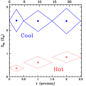
Figure 10: Radial profiles (units – bottom: arcminutes, top: kpc) of the Fe abundance and associated $1\sigma$ errors for the 2T (2D) model where the abundances have been allowed to vary separately for each component. Only shown are the the results for the inner shells.

Although the near-solar central value of the iron abundance and the values of the $\alpha$/Fe ratios provide strong evidence for SNe Ia enrichment of the hot gas from the central galaxy, there remain some problems with this scenario. First, the abundances in the hot gas generally rise toward the center and then dip in the innermost bin; this dip is more pronounced for the deprojected abundance profiles. Such a dip is difficult to understand in the context of enrichment from the central galaxy which should be most pronounced at the very center. Some cD clusters also show such a dip (e.g., Centaurus, Sanders & Fabian, 2002) which Morris & Fabian (2002) have suggested is an artifact of attempting to model a highly inhomogeneous metal distribution with a homogeneous spectral model. This model is attractive since it could explain why sub-keV cooling gas has not been found by Chandra or XMM in cooling flows.

In NGC 5044 we find that the central abundance dip is indeed sensitive to assumptions in the spectral model. (Central dips are also sensitive to the lower energy limit of the bandpass as discussed in §6.3.) If we tie oxygen to iron in their solar ratio the dip in the abundances is less pronounced. In the spirit of Morris & Fabian (2002), if instead we allow the abundances on each temperature component of the 2T model to vary separately then the abundances on the cool component remain large all the way to the center. We show the central iron abundance profile of this model in Figure 10. Because of the large number of free parameters in this model the precise radial variation of $Z_{\rm Fe}$ in Figure 10 should be treated with caution. But the basic idea that the property of a central dip is sensitive to further assumptions about the spectral model is clear.

Second, we note that although correcting for the Fe Bias partially removes the “Iron Discrepancy” noted by Arimoto et al. (1997), chemical models of elliptical galaxies without cooling flows predict central iron abundances even larger than we have measured for N5044 and NGC 1399 (Brighenti & Mathews, 2003).

It should also be emphasized that the properties of the central $\sim 5$ kpc (i.e., central $R\approx 30\arcsec$) are distinctly different from those at immediately larger radii. Hence, studies of NGC 5044 with the high-resolution gratings of Chandra and XMM can only probe this special region and cannot tell us about the properties at larger radii. We note, however, that the RGS, EPIC, and ACIS-S3 data give consistent results in their overlap regions (§6.1).

References

- Allen et al. (2000) Allen, S. W., Di Matteo, T., & Fabian, A. C. 2000, MNRAS, 311, 493
- Anders & Grevesse (1989) Anders, E. & Grevesse, N. 1989, Geochim. Cosmochim. Acta, 53, 197
- Arimoto et al. (1997) Arimoto, N., Matsushita, K., Ishimaru, Y., Ohashi, T., & Renzini, A. 1997, ApJ, 477, 128
- Awaki et al. (1994) Awaki, H., Mushotzky, R., Tsuru, T., Fabian, A. C., Fukazawa, Y., Loewenstein, M., Makishima, K., Matsumoto, H., Matsushita, K., Mihara, T., Ohashi, T., Ricker, G. R., Serlemitsos, P. J., Tsusaka, Y., & Yamazaki, T. 1994, PASJ, 46, L65
- Behar et al. (2001) Behar, E., Cottam, J., & Kahn, S. M. 2001, ApJ, 548, 966
- Brighenti & Mathews (1999) Brighenti, F. & Mathews, W. G. 1999, ApJ, 515, 542
- Brighenti & Mathews (2003) —. 2003, ApJ, 587, 580
- Buote (1999) Buote, D. A. 1999, MNRAS, 309, 685
- Buote (2000a) —. 2000a, ApJ, 539, 172
- Buote (2000b) —. 2000b, MNRAS, 311, 176
- Buote (2002) —. 2002, ApJ, 574, L135
- Buote et al. (1999) Buote, D. A., Canizares, C. R., & Fabian, A. C. 1999, MNRAS, 310, 483
- Buote & Fabian (1998) Buote, D. A. & Fabian, A. C. 1998, MNRAS, 296, 977
- Buote et al. (2003) Buote, D. A., Lewis, A. D., Brighenti, F., & Mathews, W. G. 2003, ApJ, in press (astro-ph/0205362)
- Cappellaro & Turatto (2002) Cappellaro, E. & Turatto, M. 2002, in The influence of binaries on stellar population studies ed. D. Vanbeveren (Brussels 21-25 Aug. 2000), in press (astro-ph/0012455)
- David et al. (1994) David, L. P., Jones, C., Forman, W., & Daines, S. 1994, ApJ, 428, 544
- Davis et al. (1999) Davis, D. S., Mulchaey, J. S., & Mushotzky, R. F. 1999, ApJ, 511, 34
- Finoguenov & Ponman (1999) Finoguenov, A. & Ponman, T. J. 1999, MNRAS, 305, 325
- Fukazawa et al. (1996) Fukazawa, Y., Makishima, K., Matsushita, K., Yamasaki, N., Ohashi, T., Mushotzky, R. F., Sakima, Y., Tsusaka, Y., & Yamashita, K. 1996, PASJ, 48, 395
- Gastaldello & Molendi (2002) Gastaldello, F. & Molendi, S. 2002, ApJ, 572, 160
- Gibson et al. (1997) Gibson, B. K., Loewenstein, M., & Mushotzky, R. F. 1997, MNRAS, 290, 623
- Grevesse & Sauval (1998) Grevesse, N. & Sauval, A. J. 1998, Space Science Reviews, 85, 161
- Lewis et al. (2002) Lewis, A. D., Stocke, J. T., & Buote, D. A. 2002, ApJ, 573, L13
- Loewenstein & Mushotzky (2002) Loewenstein, M. & Mushotzky, R. F. 2002, in IAU Symposium, 139
- Matsumoto et al. (1997) Matsumoto, H., Koyama, K., Awaki, H., Tsuru, T., Loewenstein, M., & Matsushita, K. 1997, ApJ, 482, 133
- Matsushita et al. (1994) Matsushita, K., Makishima, K., Awaki, H., Canizares, C. R., Fabian, A. C., Fukazawa, Y., Loewenstein, M., Matsumoto, H., Mihara, T., Mushotzky, R. F., Ohashi, T., Ricker, G. R., Serlemitsos, P. J., Tsuru, T., Tsusaka, Y., & Yamazaki, T. 1994, ApJ, 436, L41
- Matsushita et al. (2000) Matsushita, K., Ohashi, T., & Makishima, K. 2000, PASJ, 52, 685
- McWilliam (1997) McWilliam, A. 1997, ARA&A, 35, 503
- Molendi & Gastaldello (2001) Molendi, S. & Gastaldello, F. 2001, A&A, 375, L14
- Morris & Fabian (2002) Morris, R. G. & Fabian, A. C. 2002, in ASP Conf. Ser. 253: Chemical Enrichment of Intracluster and Intergalactic Medium, 85–+
- Mulchaey (2000) Mulchaey, J. S. 2000, ARA&A, 38, 289
- Mushotzky et al. (2003) Mushotzky, R., Figueroa-Feliciano, E., Loewenstein, M., & Snowden, S. L. 2003, (astro-ph/0302267)
- Nomoto et al. (1997a) Nomoto, K., Hashimoto, M., & Tsujimoto, T. 1997a, Nucl. Phys. A, 616, 79
- Nomoto et al. (1997b) Nomoto, K., Iwamoto, K., Nakasoto, N., Thielemann, F. K., Brachwitz, F., Tsujimoto, T., Kubo, Y., & Kishimoto, N. 1997b, Nucl. Phys. A, 621, 467
- Peterson & et. al. (2003) Peterson, J. R. & et. al. 2003, ApJ, submitted (astro-ph/0210662)
- Renzini (1997) Renzini, A. 1997, ApJ, 488, 35
- Renzini (2000) Renzini, A. 2000, in Large Scale Structure in the X-ray Universe, Proceedings of the 20-22 September 1999 Workshop, Santorini, Greece, eds. Plionis, M. & Georgantopoulos, I., Atlantisciences, Paris, France, p.103, 103
- Renzini et al. (1993) Renzini, A., Ciotti, L., D’Ercole, A., & Pellegrini, S. 1993, ApJ, 419, 52
- Sanders & Fabian (2002) Sanders, J. S. & Fabian, A. C. 2002, MNRAS, 331, 273
- Tamura et al. (2003) Tamura, T., Kaastra, J. S., Makishima, K., & Takahashi, I. 2003, A&A, 399, 497
- Tonry et al. (2001) Tonry, J. L., Dressler, A., Blakeslee, J. P., Ajhar, E. A., Fletcher, A. ., Luppino, G. A., Metzger, M. R., & Moore, C. B. 2001, ApJ, 546, 681
- Trager et al. (2000) Trager, S. C., Faber, S. M., Worthey, G., & González, J. J. . 2000, AJ, 119, 1645
- Wyse (1997) Wyse, R. F. G. 1997, ApJ, 490, L69
- Xu et al. (2002) Xu, H., Kahn, S. M., Peterson, J. R., Behar, E., Paerels, F. B. S., Mushotzky, R. F., Jernigan, J. G., Brinkman, A. C., & Makishima, K. 2002, ApJ, 579, 600