Abstract

We demonstrate how, with a purely empirical analysis of the irregular lightcurve data, one can extract a great deal of information about the stellar pulsation mechanism. An application to R Sct thus shows that the irregular lightcurve is the result of the nonlinear interaction of two highly nonadiabatic pulsation modes, namely a linearly unstable, low frequency mode, and the second mode that, although linearly stable, gets entrained through a 2:1 resonance. In the parlance of nonlinear dynamics the pulsation is the result of a 4 dimensional chaotic dynamics.

Nonlinear Properties of the
Semiregular Variable Stars

In the following we lump together under the label ’semiregular’ largo sensu, the stars of RV Tau type, the Semi-Regular stars and some of the Mira variables. All of these stars have lightcurves of varying degrees of irregularity. Most of our information about them comes from amateur astronomer data bases (AAVSO, AFOEV, BAAVSS and VSOLJ) which contain data on a large number of bright stars spanning almost a century. Many have at least several decades of good temporal sampling. Unfortunately, the data are very noisy, especially around the lightcurve minima, and for our analyses we therefore have to bin, smooth and filter the data to form a time-series with equal time-intervals. Figures 1 and 2, on top, show sections of lightcurves for 4 selected stars, viz. R Sct (RV Tau type), R UMi (SR type), R Cyg and X Aur (both Mira type).

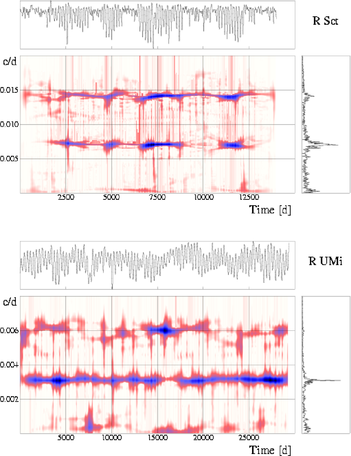
Figure 1: Time-frequency plots for R Sct and R UMi; see text for details.

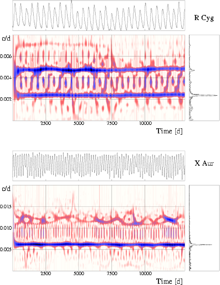
Figure 2: Time-frequency plots for R Cyg and X Aur.

The questions that we are asking here are: What are the nature and cause of the irregularities? Is there one or several underlying mechanisms? Do the the lightcurve data contain any quantitative information that can be extracted and exploited? If so, how does it correlate with luminosity, and can it be used for distance measurements? Most past work (cf. these conference proceedings) has concentrated on extracting period-luminosity relations which sheds light on the evolutionary and pulsational status and on the stellar structure of these stars. But is there additional information in the data?

Figures 1 and 2, on the right side, display the Fourier spectra of the 4 sample stars. One might be tempted to classify R UMi and X Aur as monoperiodic and R Sct and R Cyg as biperiodic as in Kiss et al. (2002). However, these stars are not multiperiodic. Neither the amplitudes, nor the phases, nor even the frequencies are constant in time. This can best be seen in the corresponding time-frequency plots. Instead of the more common wavelet or Gabor transform we have made our time-frequency plots with a Choi-Williams kernel (Cohen 1994) which has the property of sharpening features (cf. also Kolláth & Buchler 1997). It is not astonishing that the instantaneous amplitude in the dominant peak ($f_{0}$) is seen to vary (dark corresponding to higher values on the adopted greyscale), but very interestingly the instantaneous frequency varies as well! In order to make the structure of the ’harmonic’ region ($\approx 2f_{0}$) visible on the same greyscale we have scaled up the amplitudes in that region. Remarkably, the harmonic frequency does not move synchronously with the dominant frequency. Furthermore, for R Sct, the $2f_{0}$ power seems to switch back and forth between $2f_{0}$ and $2f_{0}+\Delta f$. A similar behavior occurs in X Aur.

None of these features of the time-frequency plots, nor the irregularity of the lightcurves for that matter, can be explained by evolution, by dust or spots, by binarity or by stochasticity, even though all of these effects can be present and influence the lightcurve. Instead, the time-frequency plots suggest a low dimensional underlying chaotic dynamics consisting of the nonlinear interaction of a few modes. We suggest that multimode might be a better label for these stars than multiperiodic.

In those cases where the amateur data and the Cadmus (private communication, and Buchler et al. 2002) data overlap, the time-frequency analysis gives essentially the same results - e.g. these fingerprints of nonlinear mode interactions are insensitive to observational noise.

We wish to stress that our nonlinear approach to the study of the pulsations of the semiregular stars, namely the global flow reconstruction is fully empirical, i.e. devoid of theoretical modelling. Only two working assumptions are made:

1. the lightcurve is produced by the (deterministic) nonlinear interaction of a small number of pulsation modes,

2. the system is autonomous, i.e. we ignore time dependence such as evolution over the span of the data.

For additional details we refer to Buchler & Kolláth (2000) and Buchler et al. (1996). Our assumptions imply that the star’s behavior is describable by a differential system in a physical phase space of a priori unknown dimension $d$.

$${d{\bf x}\over dt}={\bf F}({\bf x})$$ (1)

where ${\bf x}$ is a $d$-dimensional vector whose components are the phasespace variables (which could be modal amplitudes and phases, for example). For a single oscillatory mode, e.g. $d$ would be equal to 2, for 2 coupled oscillatory modes $d=4$. The involvement of a secular mode would add 1 to the dimension.

In parallel we now introduce a reconstruction space of dimension $d_{e}$, in which we construct successive position vectors

$${\bf X^{n}}=(s_{n},s_{n-\tau},s_{n-2\tau},\ldots,s_{n-(d_{e}-1)\tau})\thinspace,$$

using the observational data $s_{n}=s(t_{n})$, the magnitude in our case. The quantity $\tau$ is called the delay parameter. If our assumptions are satisfied, then the temporal behavior should be captured by an evolution equation

$${\bf X}^{n+1}={\bf\cal M}({\bf X}^{n})\thinspace,$$ (2)

provided $d_{e}$ is large enough. We could also have introduced a differential system akin to 1 in this space – our ${\bf X}^{n}$ is merely a stroboscopic description of the dynamics. The map ${\bf\cal M}$ is assumed to be a sum of all the multivariate monomials up to some order (usually 4) and the unknown coefficients are determined by a least squares fit from the data. (We minimize $||{\bf X}^{n+1}-{\bf\cal M}({\bf X}^{n})||$ over the data set). A powerful embedding theorem assures us that the dynamics in the physical phasespace and in the reconstruction space are the same provided that $d_{e}$ is large enough. Consequently, from the study the behavior of the reconstructed system we can infer otherwise unknown properties of the physical phase space.

Once we have constructed a map from the data set we can iterate that map and generate ’synthetic signals’ which are much longer than the observational data set. From the latter we can then compute Lyapunov exponents and the fractal dimension $d_{L}$. We consider a reconstruction successful when the synthetic signals are robust with respect to a range of smoothing parameters and a range of delay parameters $\tau$, are stable, and when the results are independent of the embedding dimension $d_{e}$, as long as the latter is large enough. The lowest value for which we obtain robust results will be called $d_{e}^{min}$.

In Buchler et al. (1996) we analyzed the AAVSO data of R Sct. Here we have repeated our analysis with a richer data base obtained by combining the AAVSO, AFOEV, BAAVSS and VSOLJ data and extending the basis to date. In Fig. 4 we display the R Sct lightcurve together with a typical synthetic signal in 4D. The synthetic signal is clearly seen to capture the nature of the lightcurve. This becomes even more evident when one looks at the lightcurve data over the last 150 years (Kolláth 1990). With the extended data basis our results do not change and remain very interesting.

1. In 3D no robust reconstructions are possible. The results are not changed by going to $d_{e}$ = 5 and 6. They are also independent of the delay parameter $\tau$ within a broad range. We conclude that $d_{e}^{min}=4$.

2. One of the Lyapunov exponents is always positive, implying that the pulsation is chaotic. The fractal dimension of the attractor is $d_{L}\sim 3.2$. The values of the exponents and of $d_{L}$ is largely independent of $d_{e}$.

3. Clearly the (Euclidean) dimension of the physical phasespace is sandwiched between $d_{L}=3.2$ and $d_{e}^{min}=4$. We therefore can infer that $d=4$. This suggests that the lightcurve is generated by the nonlinear interaction of two vibrational modes, consistently with the time-frequency analysis.

4. When the map is linearized around its fixed point one obtains 2 spiral stability roots $\lambda_{1}=\pm i\thinspace 0.0068\times 2\pi\thinspace+0.0044d^{-1}$, and $\lambda_{2}=\pm i\thinspace 0.0145\times 2\pi\thinspace-0.0062d^{-1}.$ Because the fixed point of the map corresponds to the equilibrium state of the star, the two spiral roots corroborate the presence and excitation of two vibrational modes. Furthermore it tells us that there is a first, linearly unstable mode of frequency $f_{0}=0.0068$ and a second mode, linearly stable one, with frequency slightly greater than $2f_{0}$. This is in agreement with the time-frequency analysis. Note that these modal properties come from a map which was obtained through a fit to the data. None of these properties were imposed.

Figure 3: R Sct: top: section of R Sct light curve; below: long synthetic signal generated with a 4D map.

We conclude that there is no need for a deus ex machina, such as irregular convective overshoots, to explain the nature of the irregular pulsations. From our empirical data analysis we have arrived at a useful physical picture: The irregular pulsation is the result of the nonlinear interaction of two strongly nonadiabatic pulsation modes. A lower frequency, linearly unstable mode entrains a stable, higher frequency one through a 2:1 resonance. The unstable mode wants to grow, but shares kinetic energy with the stable one which then dissipates it, and the cycle repeats. Because of the strongly nonadiabatic nature of these modes the motion is irregular (chaotic).

The reader may wonder why the same resonant scenario gives rise to a synchronized, periodic pulsation in the classical bump Cepheids (Buchler 1993). The physical reason is that the latter are only weakly nonadiabatic, the ratio $\eta$ of growth rate to frequency is of the order of 0.01. In the semiregulars the ratio of luminosity to mass is more than ten times larger, and $\eta$ is of order unity. The fact that the amplitude can vary on the timescale of the period is of course a necessary (but not sufficient) condition for chaotic behavior.

The amateur astronomer data bases contain a number of semiregulars with sufficient coverage to allow the same approach. We have embarked on the analysis of these stars to see if this mechanism of a resonant interaction is shared by other (most?) semiregular stars. Preliminary results for stars such as R UMi are very encouraging and again indicate a low dimensional chaotic nature of the pulsations. We also note that similar results have been obtained with high quality data (Buchler, Kolláth and Cadmus 2002). However, because our goal is to extract quantitative information, such as dimensions, Lyapunov exponents, etc., at this stage we feel that more work is necessary to establish the robustness of the results that we have obtained.

We wish to thank the organizers for their generous support which made our participation possible. Our thanks also go to the AAVSO, AFOEV, BAAVSS and VSOLJ for allowing us to use their data. This work has been supported by NSF (AST9819608) and OTKA (T038440).

1

References

- [1] Buchler, J. R. 1993, in Nonlinear Phenomena in Stellar Variability,Eds. M. Takeuti & J.R. Buchler (Kluwer: Dordrecht), repr. from ApSS 210, 1
- [2] Buchler, J. R., Kolláth, Z., Serre, T. & Mattei, J. 1996, ApJ, 462, 489
- [3] Buchler, J.R. & Kolláth, Z., 2001, ”Nonlinear Analysis of Irregular Variables”, in Nonlinear Studies of Stellar Pulsation, Eds. M. Takeuti & D.D. Sasselov, ASS Libr. Ser., 257, 185 [http://xxx.lanl.gov/abs/astro-ph/0003341].
- [4] Buchler, J.R., Kolláth, Z. & Cadmus, R. 2002, Chaos in the Music of the Spheres, Proceedings of CHAOS 2001, Potsdam, Germany, (in press); [http://xxx.lanl.gov/abs/astro-ph/0106329]
- [5] Cohen, L. 1994, Time-Frequency Analysis. Prentice-Hall PTR. Englewood Cliffs, NJ
- [6] Kolláth Z., 1990, MNRAS 247, 377
- [7] Kolláth, Z. & Buchler, J.R. (1997), Time-Frequency Analysis of Variable Star Light Curves – in Nonlinear Signal and Image Analysis, Ann. NY Acad. Sci. 808, 116.
- [8] Kiss, L.L., Szatmary, K., Cadmus, R. R. & Mattei, J.A., 1999, A&A 346, 542