Submillimeter Wave Astronomy Satellite mapping observations of water vapor around Sagittarius B2

Abstract

Observations of the $1_{10}-1_{01}$ 556.936 GHz transition of ortho-water with the Submillimeter Wave Astronomy Satellite (SWAS) have revealed the presence of widespread emission and absorption by water vapor around the strong submillimeter continuum source Sagittarius B2. An incompletely-sampled spectral line map of a region of size $26\times 19$ arcmin around Sgr B2 reveals three noteworthy features. First, absorption by foreground water vapor is detectable at local standard-of-rest (LSR) velocities in the range –100 to 0 km/s at almost every observed position. Second, spatially-extended emission by water is detectable at LSR velocities in the range 80 to 120 km/s at almost every observed position. This emission is attributable to the 180-pc molecular ring identified from previous observations of CO. The typical peak antenna temperature of 0.075 K for this component implies a typical water abundance of 1.2 – 8 $\times 10^{-6}$ relative to H₂. Third, strong absorption by water is observed within 5 arcmin of Sgr B2 at LSR velocities in the range 60 to 82 km/s. An analysis of this absorption yields a H${}_{2}^{16}$O abundance $\sim 2-4\times 10^{-7}$ relative to H₂ if the absorbing water vapor is located within the core of Sgr B2 itself; or, alternatively, a water column density of $\sim 2.5-4\times 10^{16}\,\rm cm^{-2}$ if the water absorption originates in the warm, foreground layer of gas proposed previously as the origin of ammonia absorption observed toward Sgr B2.

1 Introduction

The Sagittarius B2 cloud represents the largest condensation of molecular gas and dust in the Galaxy. With a total gas mass of $\sim 4\times 10^{6}M_{\odot}$ (Lis & Goldsmith 1989) concentrated within a region of size $\sim 30$ pc, Sgr B2 exhibits the largest submillimeter continuum flux of any astronomical source outside the solar system.

The molecular inventory of the gas in Sgr B2 has been extensively studied by means of ground-based radio observations (e.g. Cummins, Thaddeus & Linke 1986; Turner 1989, 1991; Sutton et al. 1991; Nummelin et al. 1998, 2000). Such observations have been supplemented by far-infrared and submillimeter observations carried out from airplane altitude or from space. In particular, observations carried out over the past decade with the Kuiper Airborne Observatory (KAO; see Zmuidzinas et al. 1995), the Infrared Space Observatory (ISO; see Cernicharo et al. 1997) and the Submillimeter Wave Astronomy Satellite (SWAS; see Neufeld et al. 2000) have facilitated the observation of water vapor in Sgr B2. Water is of particular interest because of its central role in the chemistry of interstellar oxygen and its potential importance as a coolant of molecular clouds (see, for example, Neufeld, Lepp & Melnick 1995; Melnick et al. 2000; Bergin et al. 2000).

In a earlier study of Sgr B2, we used SWAS to obtain the first high-spectral-resolution ($\Delta v\sim 1{\rm\,km\,s^{-1}}$) observations of H${}_{2}^{16}$O toward that source. In a previous paper (Neufeld et al. 2000; hereafter N00), we reported the detection of water absorption over a wide range of LSR velocities that can be attributed to water vapor in foreground clouds that are not associated with Sgr B2. We have since extended these observations to map (incompletely) a region of size $26^{\prime}\times 19^{\prime}$ around Sgr B2. In the present paper, we describe these new mapping observations and discuss the abundance of water vapor in the vicinity of Sgr B2 itself.

2 Observations

Our mapping observations of Sagittarius B2 were carried out during the period 1999 March 20 through 2000 September 16. They yielded incomplete coverage of a region extending $9.6^{\prime}$ North, South and East and $16.0^{\prime}$ West of Sagittarius B2. In Table 1 we list the on-source integration times for each of 19 positions observed, together with the offsets relative to the core of Sgr B2 at position $\rm\alpha=17^{h}\,47^{m}\,19.^{s}7$, $\delta=-28^{\circ}23^{\prime}07^{\prime\prime}$ (J2000). At 550 GHz the SWAS beam size is $3.3^{\prime}\times 4.5^{\prime}$ and the main beam efficiency is 0.9 (Melnick et al. 2000). All the data were acquired in standard nodded observations (Melnick et al. 2000) and were reduced using the standard SWAS pipeline. The reference (nod) position was located at $\rm\alpha=17^{h}\,54^{m}\,12.^{s}2$, $\delta=-29^{\circ}42^{\prime}19^{\prime\prime}$ (J2000) in a region of devoid of strong CO emission. The total on-source integration time for these mapping observations was 90.4 hours.

Because SWAS employs double-sideband receivers, the ¹³CO $J=5-4$ transition at 550.927 GHz and the H₂O $1_{10}-1_{01}$ transition at 556.936 GHz are observed simultaneously in the lower and upper sidebands of one receiver (Receiver 2). For the mapping observations, the SWAS local oscillator (LO) setting was chosen to separate the ¹³CO emission from Sgr B2 (at $v_{\rm LSR}\sim 65\,\rm km\,s^{-1}$) from any H₂O emission or absorption at LSR velocities $v_{\rm LSR}\geq 0$. For the (0,0) position, several additional LO settings had previously been used (see N00) to allow the region $-145{\rm\,km\,s^{-1}}\leq v_{\rm LSR}\leq 0{\rm\,km\,s^{-1}}$ to be covered as well without contamination by ¹³CO emission from the lower sideband.

3 Results

In Figure 1, we show the nineteen H₂O spectra obtained from our mapping observations described above. Each panel shows a spectrum covering the range $-145{\rm\,km\,s^{-1}}\leq v_{\rm LSR}\leq 145{\rm\,km\,s^{-1}}$. The vertical dotted line denotes $v_{\rm LSR}\sim 65\,\rm km\,s^{-1}$, the systemic velocity of Sgr B2. The upper horizontal dotted lines indicate the continuum flux level, determined from the spectral regions $v_{\rm LSR}=-145$ to $-125\,\rm km\,s^{-1}$ and 125 to 145$\,\rm km\,s^{-1}$ that are devoid of absorbing gas, and the lower horizontal dotted lines indicate the zero flux level, estimated by the method described in §4.1 below. On each panel a pair of numbers, X/Y, describe respectively the continuum antenna temperature (which corresponds to the separation between the two dotted horizontal lines), and the antenna temperature (in K) at the top of the panel. The former is also given in Table 1.

The feature at $v_{\rm LSR}\sim-90$ to $-50\,\rm km\,s^{-1}$ is a ¹³CO emission feature detected in the lower sideband. In Figure 2, we show the Receiver 2 data reduced as appropriate for the ¹³CO line in the lower sideband; a strong feature at $v_{\rm LSR}\sim 65\,\rm km\,s^{-1}$ is observed at several positions close to Sgr B2. We note that the spectra in Figure 2 are not perfect mirror images of those shown in Figure 1; in particular, the ¹³CO features are significantly narrower in the spectra that were reduced as appropriate for the lower sideband (Figure 2). The reason for this behavior is that the SWAS LO setting is fixed in the rest frame of the spacecraft, which has a motion relative to the local standard of rest (LSR) that varies quite rapidly. In particular, the spacecraft orbits the Earth every 97 minutes with an orbital speed of $7\,\rm km\,s^{-1}$ (and – of course – the Earth also orbits the Sun.) In the standard SWAS pipeline, the necessary Doppler corrections are applied to every 2 seconds’ worth of data, and the sign of the correction is opposite for the lower and upper sidebands. Thus any spectral line originating in the lower sideband will be smeared out as it appears in Figure 1, while any line from the upper sideband will appear broadened in Figure 2.

Although not the primary emphasis of this paper, for completeness we present additional spectra obtained for the $\rm{}^{3}P_{1}-^{3}P_{0}$ fine structure line of atomic carbon. These spectra, shown in Figure 3, are obtained from Receiver 1 (upper sideband) on the SWAS instrument, which performs simultaneous observations of the CI $\rm{}^{3}P_{1}-^{3}P_{0}$ line in a linear polarization orthogonal to that observed with Receiver 2. There is no evidence for emission or absorption by the 487.249 $3_{1}-3_{2}$ transition of O₂, to which Receiver 1 is sensitive in its lower sideband.

4 Discussion

Even a cursory inspection of Figure 1 reveals three significant features in the water spectra: (1) extended absorption, observed at almost every one of the 19 positions, covering the range $-100\,{\rm km\,s^{-1}}\lower 2.15277pt\hbox{$\;\buildrel<\over{\sim}\;$}v_{\rm LSR}\lower 2.15277pt\hbox{$\;\buildrel<\over{\sim}\;$}0$; (2) extended emission, again observed at almost every position, covering the range $80\lower 2.15277pt\hbox{$\;\buildrel<\over{\sim}\;$}v_{\rm LSR}\lower 2.15277pt\hbox{$\;\buildrel<\over{\sim}\;$}120\,{\rm km\,s^{-1}}$; (3) less-extended absorption, only observed unequivocally at the $(0.0^{\prime},0.0^{\prime})$, $(0.0,+3.2^{\prime})$, $(0.0,-3.2^{\prime})$, $(-3.2^{\prime},0.0)$ and $(-3.2^{\prime},-3.2^{\prime})$ positions, centered at v${}_{\rm LSR}\sim 65\,{\rm km\,s^{-1}}$, the systemic velocity of the Sgr B2 cloud.

4.1 Extended absorption by water vapor at $\bf v_{\bf LSR}\sim 0\,km\,s^{-1}$

Broad absorption by water vapor over the entire velocity range $v_{\rm LSR}$ = –100 to $0\,\rm km\,s^{-1}$ has been inferred previously from SWAS observations of H${}_{2}^{16}$O and H${}_{2}^{18}$O toward Sgr B2 (N00; see also Figure 7), the H${}_{2}^{18}$O spectrum indicating that the peak optical depth occurs at $v_{\rm LSR}\sim 0$. The absorption in this velocity range can be attributed to material lying at a wide range of locations along the line-of-sight between the Solar circle and Sgr B2.

The mapping observations presented in Figure 1 show clear evidence for absorption at $v_{\rm LSR}\sim 0\,\rm km\,s^{-1}$ at 18 of the 19 positions observed, implying that both the continuum emission and intervening material have a large angular extent. The angular extent of the absorbing water vapor at $v_{\rm LSR}\sim 0$ is considerably larger than that of the water vapor at $v_{\rm LSR}\sim 65{\rm\,km\,s^{-1}}$, the systemic velocity of Sgr B2. The large spatial extent of the water absorption at $v_{\rm LSR}\sim 0\,\rm km\,s^{-1}$ is further demonstrated by the SWAS spectrum of water vapor toward Sgr A, shown in Figure 4, which clearly exhibits strong absorption in this velocity range. Located at position $\rm\alpha=17^{h}\,45^{m}\,39.^{s}7$, $\delta=-29^{\circ}00^{\prime}30^{\prime\prime}$ (J2000), SgrA is at offset (–21.8^′, –37.4^′) relative to Sgr B2. Thus the SWAS observations of the Galactic Center region show water absorption at $v_{\rm LSR}\sim 0\,\rm km\,s^{-1}$ covering a region of longest angular dimension 50 arcmin, corresponding to a linear scale of 125 pc for an assumed distance to the Galactic Center of 8.5 Kpc. Of course, if the absorbing material lies significantly closer to us than the Galactic Center, then its linear extent could be smaller than 125 pc.

The presence of strong absorption at $v_{\rm LSR}\sim 0$ allows us to estimate the continuum flux level, a quantity that is not reliably determined by the SWAS instrument. In particular, the zero flux level in Figure 1 and Table 1 is established on the assumption that the spectral region $v_{\rm LSR}=$ –5 to 5$\,\rm km\,s^{-1}$ is subject to complete absorption by water vapor in foreground material along the line-of-sight to Sgr B2. This assumption is motivated by the facts that (1) absorption at $v_{\rm LSR}\sim 0\,\rm km\,s^{-1}$ is observed at almost every position and is well separated from contamination from ¹³CO emission in the lower sideband; and (2) the H${}_{2}^{18}$O spectrum of the $1_{10}-1_{01}$ line at the (0.0^′,0.0^′) position (see N00; also Figure 7) implies an optical depth $\sim 1$ at $v_{\rm LSR}\sim 0$, corresponding to an H${}_{2}^{16}$O $1_{10}-1_{01}$ optical depth of several hundred. If the $v_{\rm LSR}=$ –5 to 5$\,\rm km\,s^{-1}$ spectral region is not subject to complete absorption, then the continuum antenna temperatures quoted are lower limits.

The continuum antenna temperatures obtained by this method can be compared with continuum maps presented by Dowell et al. (1999), who observed Sgr B2 with the SHARC instrument at the Caltech Submillimeter Observatory. In Table 1, we show the 350 $\mu$m continuum fluxes (in kJy per SWAS beam) – obtained by convolving the SHARC data with the SWAS beam profile – along with the SWAS-determined 550 GHz ( 540 $\mu$m) continuum fluxes. The SHARC-measured 350 $\mu$m continuum fluxes should be regarded as lower limits because the relatively small offset of only 2 arcmin for the SHARC reference beam (Dowell, private communication) can lead to highly extended emission being “chopped out”. Toward the central 9 positions [i.e. the (0,0) position and 8 positions closest to it], the inferred 540 $\mu$m / 350 $\mu$m continuum flux ratios all lie in the range 0.17 to 0.42. We have compared these values with those expected for optically-thin dust with an opacity that varies as $\lambda^{-2}$. The ratios observed toward the central nine positions are all consistent with dust temperatures of 15 K and above; the larger values of the 540 $\mu$m / 350 $\mu$m flux ratio observed at greater distances from the cloud center suggest that the dust temperature is smaller in the outer parts of the Sgr B2 cloud.

4.2 Extended emission from water vapor in the 180-pc molecular ring ($\bf v_{\bf LSR}\sim 80-120\,\bf km\,s^{-1}$)

Extended water emission in the $v_{\rm LSR}\sim 80-120\,\rm km\,s^{-1}$ velocity range is detected from 18 of the 19 positions we observed in the vicinity of Sgr B2, with the integrated antenna temperatures given in Table 2. Emission in this velocity range is also evident in the spectrum of Sgr A (Figure 4), although it is blended with a strong emission feature centered at $v_{\rm LSR}\sim 65\,\rm km\,s^{-1}$. In Figure 5, we show the average spectrum for those 14 positions near Sgr B2 that are devoid of apparent absorption at the Sgr B2 systemic velocity. The solid line is Gaussian fit to the average emission feature: its velocity centroid is $\rm 93\,km\,s^{-1}$, the line width is $\rm 43\,km\,s^{-1}$, the peak antenna temperature is 0.075 K, and the velocity-integrated antenna temperature is $3.4\rm\,K\,km\,s^{-1}$.

This extended emission feature is kinematically similar to a highly extended emission component detected in ¹³CO maps of the Galactic Center region (Bally et al. 1987; Lis & Goldsmith 1989, hereafter LG89). It arises from the far side of a molecular ring of angular diameter $\sim$ 2 degrees – corresponding to a projected radius of $\sim 180$ pc – the near side of which shows ¹³CO emission and H₂O absorption (N00) at negative LSR velocities. The kinematic properties of this 180-pc molecular ring yield a parallelogram in the $l-v$ plane; they have been attributed either to an explosion-driven expansion (Scoville 1972; Kaifu et al. 1972) or – more recently – to the gravitational effects of a Galactic bar potential (Binney et al. 1991).

In Table 2, we also show the H₂O $1_{10}-1_{01}$ / ¹³CO $J=1-0$ line ratio for each of the SWAS observed positions. The ¹³CO $J=1-0$ spectra were obtained by convolving the map of Bally et al. (1987) with the SWAS beam profile, approximated as a Gaussian circular beam of diameter 4 arcmin (FWHM). For the 14 positions that are devoid of apparent absorption at the Sgr B2 systemic velocity, the line ratios apply to the velocity range $v_{\rm LSR}=80-120\,\rm km\,s^{-1}$. For the other 5 observed positions, the line ratios apply only to emission redward of the average H₂O line centroid, i.e. to the velocity range $v_{\rm LSR}=93-120\,\rm km\,s^{-1}.$ The reason for restricting the velocity range for these positions is to avoid any effects of the Sgr B2 water absorption line upon the line ratios derived for the extended emission feature.

With the exception of a single position at which the H₂O $1_{10}-1_{01}$ line was not detected, the H₂O $1_{10}-1_{01}$ / ¹³CO $J=1-0$ line ratio lies within a factor 2 of 0.065. In order to estimate the water abundances implied by the observed H₂O $1_{10}-1_{01}$ / ¹³CO $J=1-0$ line ratios, we have made use of a statistical equilibrium calculation for the line strengths. We adopted the rate coefficients of Flower & Launay (1985) for collisional excitation of CO by H₂, and those of Phillips, Maluendes & Green (1996) for that of H₂O by H₂. Our excitation model indicates that the ¹³CO $J=1-0$ line is optically thin and that the H₂O $1_{10}-1_{01}$ is effectively thin. Thus the inferred H₂O to ¹³CO abundance ratio is proportional to the H₂O $1_{10}-1_{01}$ / ¹³CO $J=1-0$ line ratio.

The inferred H₂O to ¹³CO abundance ratio also depends upon the conditions of temperature and density assumed for the emitting region. Based upon multitransition observations of CO using the AST/RO telescope, Kim et al. (2002) have argued that the physical conditions within a few hundred parsec of the Galactic Center are remarkably constant – except within the Sgr A and Sgr B regions themselves – with the gas temperature everywhere in the range 30 to 45 K and the H₂ density in the range 2500 to 4000 $\rm cm^{-3}$. Given these ranges of temperature and density, we find that the ortho-H₂O/¹³CO abundance ratio is a factor of 4 – 27 times as large as the H₂O $1_{10}-1_{01}$ / ¹³CO $J=1-0$ line ratio. The typical observed H₂O $1_{10}-1_{01}$ / ¹³CO $J=1-0$ line ratio of 0.065 therefore implies an ortho-H₂O/¹³CO abundance ratio of 0.26 to 1.8. Assuming a ¹²CO abundance of 10^-4 relative to H₂, a ¹²CO/¹³CO abundance ratio of 30 for Galactic Center material (Langer & Penzias 1990), and an ortho-to-para ratio of 3 for water vapor, we obtain a value of 1.2 – 8 $\times 10^{-6}$ for the typical total water abundance relative to H₂ within the “180-pc” molecular ring.

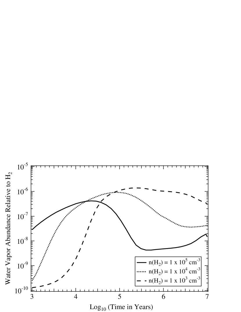
Figure 6: Water vapor abundance as a function of time for three different H₂ densities. Model results are predicted using the gas-grain model with limited surface chemistry presented by Bergin et al. (2000). The gas is assumed to be completely shielded from external ultraviolet radiation and to have a temperature of 10 K.

These water abundances inferred for the low density gas responsible for the $v_{\rm LSR}\sim 80-120\,\rm km\,s^{-1}$ extended water emission are two to four orders of magnitude larger than those measured within cold dense molecular clouds (e.g. Snell et al. 2000). Thus the results obtained here from observations of water emission confirm our previous conclusion (N00) – based upon absorption line observations – that the water abundance is typically larger in low-density interstellar gas. The most plausible explanation lies in the density dependence of the water vapor abundance, which is illustrated in Figure 6. This figure shows model predictions from the gas-grain model presented by Bergin et al. (2000) for three different molecular hydrogen densities. For lower densities the longer depletion timescales allow water vapor to exist in higher abundance. In dense regions, the abundance of water vapor is suppressed more rapidly by the depletion of oxygen nuclei onto icy grain mantles (Bergin et al. 2000).

4.3 Water abundance in Sagittarius B2

In a previous paper (N00), we published the spectra of H₂O and H${}_{2}^{18}$O $1_{01}-1_{01}$ transitions obtained toward the $(0,0)$ position and shown here in Figure 7. Now that the general properties (i.e. velocity centroid and line width) of the extended 80 – 120 $\rm\,km\,s^{-1}$ emission have been elucidated, we return to a consideration of the H₂O and H${}_{2}^{18}$O $1_{01}-1_{01}$ absorption features at $v_{\rm LSR}\sim 65\,\rm km\,s^{-1}$.

We have attempted to fit the SWAS-observed absorption at the $(0,0)$ position with the use of two models. In the first model, we follow Zmuidzinas et al. (1995, hereafter Z95; see also Neufeld et al. 1997) in assuming that the absorbing water vapor is mixed with the continuum-emitting dust in the core of Sgr B2 itself; whereas in the second model, we assume the water vapor to lie in separate intervening clouds – located close to Sgr B2 – that partially cover the continuum emission (see Ceccarelli et al. 2002).

4.3.1 Water vapor in the core of Sgr B2

In modeling the core of Sgr B2, we made use of a radiative transfer code very kindly made available by J. Zmuidzinas. This code yields a solution to the equations of statistical equilibrium for the water level populations – as a function of position within a spherically-symmetric, dusty, molecular cloud core – using the method of Accelerated Lambda Iteration (ALI) to obtain a converged, self-consistent solution to the level populations and the radiation field. Ray tracing is then used to determine the spectrum observed by a telescope with a Gaussian beam profile of specified projected diameter. The density in the core of Sgr B2 was assumed to follow the profile of LG89, Model C, and the temperature of the gas and dust to follow the profiles assumed by Z95. The total continuum opacity was adjusted to match the observed (optically-thin) continuum emission at 550 GHz, with $\tau$ assumed to vary with wavelength as $\lambda^{-1.5}$. We adopted the values given by Phillips, Maluendes & Green (1996) for the rate coefficients for excitation of H₂O in collisions with H₂, assuming an local thermodynamic equilibrium (LTE) ortho-to-para ratio for H₂. The excitation model included the lowest 8 states of ortho-H₂O.

In fitting the SWAS-observed H${}_{2}^{18}$O line, we varied three parameters: the microturbulent line width in the cloud core, the H${}_{2}^{18}$O abundance, and the velocity centroid relative to the LSR. All three were assumed to be constant throughout the cloud core. The blue curve in Figure 7 (lower panel) shows the best fit to the H${}_{2}^{18}$O absorption at $v_{\rm LSR}\sim 65\rm\,km\,s^{-1}$ obtained by this method. The best-fit microturbulent line width is $20{\rm\,km\,s^{-1}}$, the ortho-H${}_{2}^{18}$O abundance is $6.4\times 10^{-10}$ relative to H₂, and the LSR velocity centroid is $64{\rm\,km\,s^{-1}}$. Assuming an H${}_{2}^{16}$O/H${}_{2}^{18}$O abundance ratio of 250 (N00; Langer & Penzias 1990), and a water ortho-to-para ratio of 3, we derive a total H${}_{2}^{16}$O abundance of $2.1\times 10^{-7}$ relative to H₂. This derived abundance is in acceptable agreement with the value of $3.3\times 10^{-7}$ derived previously (Z95) from KAO observations of H${}_{2}^{18}$O and reported by N00.

In the upper panel of Figure 7, the blue curve shows the fit to the H${}_{2}^{16}$O absorption at $v_{\rm LSR}\sim 65{\rm\,km\,s^{-1}}$, for the water abundance, line width and centroid velocity given above. One additional free parameter is introduced here: the peak antenna temperature (taken as 0.18 K in this fit) of an emission component with the line centroid and line width derived in §3.4 above for the “180-pc molecular ring”. The fit to the H${}_{2}^{16}$O absorption (upper panel, Figure 7, blue curve) is clearly deficient in three regards: (1) the predicted absorption line is too broad; (2) the predicted absorption line is too deep, and (3) the predicted emission peaks at $v_{\rm LSR}=33$ and $95{\rm\,km\,s^{-1}}$ are not observed.

The first of these deficiencies is a direct consequence of the simplified velocity structure assumed in this model. Observations of ammonia absorption towards Sgr B2 (e.g. Hüttemeister et al. 1995, hereafter H95) have revealed the presence of three distinct absorption components in the $v_{\rm LSR}=60$ to $70{\rm\,km\,s^{-1}}$ interval (see discussion in the next subsection). Although none of these components shows a line width greater than $\sim 12{\rm\,km\,s^{-1}}$ (FWHM), collectively they blend to impart an overall line width $\sim 20{\rm\,km\,s^{-1}}$ (FWHM) to optically-thin absorption lines. For the optically-thick H${}_{2}^{16}$O line, however, the observed line width does not increase as rapidly as it would for a single Gaussian component.

Taken at face value, the second deficiency – the fact that the observed H₂O line is less deep than the model predicts – would imply that the H${}_{2}^{16}$O abundance is much less than assumed in the model. In Figure 8, middle panel, we show the line-center flux-to-continuum-flux ratio – as predicted by the Zmuidzinas radiative transfer code – as a function of the assumed water abundance. The observed ratio $\sim 0.25$ would imply an H${}_{2}^{16}$O abundance of only $\sim 2\times 10^{-9}$ and a very small H${}_{2}^{16}$O/H${}_{2}^{18}$O ratio of $\sim 3$. We are aware of no chemical fractionation mechanism capable of yielding such a small H${}_{2}^{16}$O/H${}_{2}^{18}$O ratio. A far more likely explanation of the anomalous depth of the H${}_{2}^{16}$O absorption feature is that some fraction ($\sim 25\%$) of the continuum emission detected in the SWAS beam originates in material with a very small water abundance (and which is not covered by any intervening cloud containing water). The likely presence of continuum emission that is not covered by a significant water column density has implications for the H${}_{2}^{18}$O abundance obtained above. For the water-covered component, the effective line-center to continuum ratio decreases from 0.49 to $(0.49-0.25)/0.75=0.32$, and the implied ortho-H${}_{2}^{18}$O abundance increases by a factor of almost $2$ from $6.4\times 10^{-10}$ to $1.1\times 10^{-9}$. Given the same ortho-to-para and H${}_{2}^{16}$O/H${}_{2}^{18}$O ratios assumed previously, this corresponds to a total H${}_{2}^{16}$O abundance of $3.7\times 10^{-7}$. Therefore, we conservatively adopt the range $2-4\times 10^{-7}$ as the H${}_{2}^{16}$O abundance implied by our model of the Sgr B2 core.

The third deficiency of the simple model we considered is its prediction of narrow emission peaks at $v_{\rm LSR}=35$ and $95{\rm\,km\,s^{-1}}$; this again is inconsistent with observed spectrum. A “double-horned” structure is predicted because the $1_{10}-1_{01}$ resonance-line photons that are excited collisionally within the cloud core are scattered significantly in frequency before they can escape the cloud. The top and bottom panels in Figure 8 show the predicted line-to-continuum ratios in these peaks and the predicted frequency offsets from line center (in velocity units).

The observed absence of the blue-shifted horn is naturally explained by the known presence of foreground absorbing material at $v_{\rm LSR}\sim 33{\rm\,km\,s^{-1}}$. The absence of a red-shifted horn could easily be explained if the velocity dispersion increases slightly with increasing distance from the core center; such an increase would lead to the red-horn photons being spread over an spatially-extended region, leading to a decrease in the observed surface brightness relative to what is predicted by our constant velocity-dispersion model (see discussion in N00).

4.3.2 Water vapor in an intervening cloud

As an alternative means of interpreting the H₂O and H${}_{2}^{18}$O absorption towards the $(0,0)$ position in Sgr B2, we have fitted the spectrum with a series of absorption features that are assumed to originate in foreground molecular gas outside the core of Sgr B2. In this picture – favored by H95 and by Ceccarelli et al. (2002; hereafter C02) for the origin of the NH₃ absorption observed toward Sgr B2 – the absorption originates in warm, low-density gas located outside the central core of Sgr B2 itself. According to C02, ISO observations of far-infrared NH₃ absorption lines imply a gas temperature $\sim 700$ K, while the absence of observable far-IR CO emission places an upper limit $n({\rm H}_{2})\lower 2.15277pt\hbox{$\;\buildrel<\over{\sim}\;$}3\times 10^{3}\rm\,cm^{-3}$ on the gas density; in the best-fit model of C02, the warm absorbing gas is located at a distance $\sim 1.15$ pc from the center of the Sgr B2 core.

In fitting the SWAS-observed H₂O and H${}_{2}^{18}$O spectra in this picture, we adopted the absorption line parameters derived by H95 from high resolution observations of NH₃ absorption lines. Those observations were carried out separately toward two condensations within the Sgr B2 cloud: Sgr B2(N) and Sgr B2(M). These condensations, which are separated by $\sim 0.8^{\prime}$, are not resolved individually by the $3.3^{\prime}\times 4.5^{\prime}$ SWAS beam. H95 observed absorption components at $v_{\rm LSR}=60.4$ and $69.0{\rm\,km\,s^{-1}}$ toward Sgr B2(M) but not Sgr B2(N), and absorption components at $v_{\rm LSR}=66.7$ and $81.5{\rm\,km\,s^{-1}}$ toward Sgr B2(N) but not Sgr B2(M). The line widths and NH₃ column densities inferred by H95 for these absorption components are listed in Table 3.

We regarded the velocity centroids and line widths for these four components to be fixed in our fitting of the SWAS-observed H₂O and H${}_{2}^{18}$O spectra. We took as adjustable parameters the following: (1) the fraction, $f_{A}$, of the continuum emission covered by the 60.4 and $69.0{\rm\,km\,s^{-1}}$ clouds; (2) the fraction $f_{B}$, of the continuum emission covered by the 66.7 and $81.5{\rm\,km\,s^{-1}}$ clouds; (3) the strength of the 80 – 120${\rm\,km\,s^{-1}}$ emission feature at the $(0,0)$ position in Sgr B2 (with an assumed line centroid and width as derived from the average spectrum shown in Figure 5 and discussed in §4.2); (4) the H${}_{2}^{18}$O line center optical depths in each of the four absorption components. Following C02, the absorption was considered to occur in a “foreground screen”.

As in §4.3.1, we assumed an H${}_{2}^{16}$O/H${}_{2}^{18}$O abundance ratio of 250, and a water ortho-to-para ratio of 3. In the upper panel of Figure 7, the red curve shows our best fit to the H${}_{2}^{16}$O absorption using this model. Because the H${}_{2}^{16}$O lines have optical depths of several hundred and therefore lie on the flattest part of the curve-of-growth, the H${}_{2}^{16}$O spectrum is almost entirely insensitive to the assumed optical depth; it therefore provides a relatively unambiguous determination of the covering factors $f_{A}$ and $f_{B}$. The red curve represents our best fit to the H${}_{2}^{16}$O spectrum, obtained for $f_{A}=0.6$, $f_{B}=0.2$, and with a 80 – $120{\rm\,km\,s^{-1}}$ emission feature of peak antenna temperature 0.2 K.

Once the covering factors have been determined from the H${}_{2}^{16}$O spectrum, the line-center optical depths can be determined from the H${}_{2}^{18}$O spectrum. The red curve in the lower panel of Figure 7 represents our best fit to the data, obtained with line-center optical depth of 1.3, 1.0, 0.8, and 1.5 respectively for the $v_{\rm LSR}=60.4$, 66.7, 69.0, and $81.5{\rm\,km\,s^{-1}}$ features.

ISO observations of the $2_{21}-1_{10}$ transition of H${}_{2}^{16}$O at 108.073 $\mu$m yield a further observational constraint upon the material responsible for the water absorption. A Long-Wavelength Spectrometer Fabry-Perot spectrum of the source (Goicoechea & Cernicharo 2003) yields an absorption line equivalent width $\sim 20{\rm\,km\,s^{-1}}$. Using a simple excitation model to estimate the fractional populations of the H${}_{2}^{16}$O rotational states, we find the observed 108 $\mu$m equivalent width to be consistent with the best-fit optical depths and covering factors derived from the SWAS observations (Table 3). Unfortunately, the 108 $\mu$m line lies on the flat part of the curve-of-growth, so the observed equivalent width does not place strong constraints upon the physical conditions in the absorbing material.

The absorbing column densities implied by the H${}_{2}^{18}$O line-center depths are inversely proportional to the difference $f_{01}-f_{10}$, where $f_{01}$ is the fraction of ortho-water molecules in the 1₀₁ rotational state and $f_{10}$ is the fraction in 1₁₀. Thus the minimum column density of H${}_{2}^{18}$O is obtained for the assumption $f_{01}=1$, $f_{10}=0$; these minimum values are tabulated in Table 3. The beam-averaged, minimum total column density – weighted by the continuum antenna temperature – is $N({\rm H_{2}^{18}O})=1.0\times 10^{14}\rm\,cm^{-2}$, a value in excellent agreement with the value of $1.1\times 10^{14}\rm\,cm^{-2}$ derived previously for the minimum H${}_{2}^{18}$O column density from KAO observations by Z95. The actual column density is larger by a factor $(f_{01}-f_{10})^{-1}$.

We have used a statistical equilibrium model for the H${}_{2}^{18}$O level populations to estimate the correction factor $(f_{01}-f_{10})^{-1}$. In Figure 9, we plot the values of $f_{01}$, $f_{10}$ and their difference $f_{01}-f_{10}$ as a function of the radiation field. Here we follow C02 in assuming that the far-infrared continuum radiation originates in a region of radius $R_{\rm FIR}$ = 0.8 pc, and determine the H${}_{2}^{18}$O level populations as a function of the “dilution factor”, $W$. The spectral shape of the far-infrared continuum source was obtained from Pipeline-10 archived ISO LWS grating spectra and re-processed using the ISO Spectroscopic Analysis Package version 2.1. The dilution factor is defined such that the solid angle subtended by the far-infrared continuum source is $4\pi W$ at the location of the absorbing water vapor. It is related to the distance, $R$, from the center of Sgr B2 (top horizontal axis in Figure 9) by the expression $W=\textstyle{1\over 2}\displaystyle[1-(1-R_{\rm FIR}^{2}/R^{2})^{1/2}]$. Solid curves in Figure 9 show results for the temperature and density favored by C02 for the absorbing material: an H₂ density of $3\times 10^{3}\rm\,cm^{-3}$ and a gas temperature of 700 K. Dotted curves show the results obtained for the same assumed temperature but with the density increased by a factor of 10.

Two features of Figure 9 are noteworthy. First, the level populations are not greatly affected by a factor 10 increase in the assumed density. This behavior is explained by the fact that the gas density is very much smaller than the “critical density” for the $1_{10}-1_{01}$ transition; the excitation of this transition is therefore controlled by the radiation field. Second, the quantity $f_{01}-f_{10}$ is close to unity unless the absorbing material is located very close to the center of the Sgr B2 core. For the distance of 1.15 pc favored by C02, corresponding to $W=0.15$, the value of $f_{01}-f_{10}$ is 0.8 and the correction factor $(f_{01}-f_{10})^{-1}$ is only 1.25. Significantly smaller values of the distance of the absorbing material from the cloud core are ruled out by the requirement that the absorbing water vapor must lie in front of most of the emitting dust. We conservatively adopt an upper limit of 1.5 for the correction factor $(f_{01}-f_{10})^{-1}$.

Using the analysis method of §4.3.2, where the water absorption is assumed to arise in a foreground cloud of warm, low-density material, our estimate of the beam-averaged H${}_{2}^{18}$O column density lies in the range $1.0-1.5\times 10^{14}\,\rm cm^{-2}$. Given an assumed abundance ratio of 250 for H${}_{2}^{16}$O/H${}_{2}^{18}$O, the H${}_{2}^{18}$O column density we derived implies an H${}_{2}^{16}$O column density of $2.5-4\times 10^{16}\rm\,cm^{-2}$. The total H₂ column density of the warm absorbing gas layer is not well constrained by observations; if we adopt the estimate of $10^{22}\rm\,cm^{-2}$ given by Flower et al. (1995), then the water abundance is a few $\times 10^{-6}$.

As noted by Flower et al. (1995) – and contrary to the assertion of C02 that there is no discrepancy – the observed water column density lies an order of magnitude below the predictions of shock models for the warm, absorbing gas layer in front of Sgr B2. Recent observations of high OH abundances in Sgr B2 (Goicoechea & Cernicharo 2002) may provide an explanation of the discrepancy between theory and observation. As suggested by Goicoechea & Cernicharo, if the shocked gas is irradiated by strong ultraviolet radiation from a population of hot stars, then photodissociation will reduce the H₂O abundance and increase the OH abundance. Further chemical modeling is needed, however, to determine whether this explanation is either quantitatively plausible or consistent with the large observed abundance of NH₃ in the absorbing gas.

4.3.3 Summary: water vapor in the cold core or in a warm intervening cloud?

In §4.3.1 and §4.3.2 above, we have used two alternative methods to analyse the SWAS observations of H${}_{2}^{16}$O and H${}_{2}^{18}$O at the $(0,0)$ position in Sgr B2. Although the first method – in which the water vapor and dust are assumed to be well mixed in the cloud core – yields a fit to the data which is inferior to that of the second method – in which the water vapor is assumed to lie in a foreground gas cloud – the poorer fit can be ascribed to the fact that the assumed velocity structure was far simpler in the first analysis method. On the basis of the SWAS data alone, therefore, we do not find compelling evidence to favor one picture over the other.

In principle, both the cold core and a warm intervening cloud might contribute to the observed water absorption. Insofar as the water column densities involved add linearly, we may conclude that

$$\biggl{(}{N_{\rm fg}(\rm{H_{2}O})\over{\rm 2.5\,to\,4\times 10^{16}cm^{-2}}}\biggr{)}+\biggl{(}{x_{\rm c}(\rm{H_{2}O})\over\rm 2-4\times 10^{-7}}\biggr{)}\sim 1$$

where $N_{\rm fg}(\rm{H_{2}O})$ is the water column density in the warm foreground material and $x_{\rm c}(\rm{H_{2}O})$ is the water abundance relative to H₂ in the core. Clearly, we may regard $4\times 10^{16}\,\rm cm^{-2}$ and $4\times 10^{-7}$ as conservative upper limits on $N_{\rm fg}(\rm{H_{2}O})$ and $x_{\rm c}(\rm{H_{2}O})$.

Figure 1: SWAS spectra of the 556.936 GHz $1_{10}-1_{01}$ transition of H${}_{2}^{16}$O, observed in the vicinity of Sgr B2. Each panel covers the LSR velocity range $-145$ to $145{\rm\,km\,s^{-1}}$. Adjacent spectra are offset by $3.2^{\prime}$. Horizontal dotted lines indicate the the continuum flux level and the zero flux level. The vertical dotted lines indicate a LSR velocity of 65$\,\rm km\,s^{-1}$. On each panel, a pair of numbers, X/Y, describe, in order, the continuum antenna temperature and the antenna temperature (in K) at the top of the panel. The feature at $v_{\rm LSR}\sim-90$ to $-50\,\rm km\,s^{-1}$ is a ¹³CO emission feature detected in the lower sideband. The (0,0) position is in the middle of the central group of nine spectra.

Figure 2: SWAS spectra of the 550.927 GHz $J=5-4$ transition of ¹³CO, observed in the vicinity of Sgr B2. Each panel covers the LSR velocity range $-145$ to $145{\rm\,km\,s^{-1}}$. The vertical dotted lines indicate a LSR velocity of 65$\,\rm km\,s^{-1}$. Adjacent spectra are offset by $3.2^{\prime}$. The number on each panel gives the antenna temperature (in K) at the top of the panel. The feature at $v_{\rm LSR}\sim-120$ to $-80\,\rm km\,s^{-1}$ is H₂O emission being detected in the upper sideband. The (0,0) position is in the middle of the central group of nine spectra.

Figure 3: Same as Figure 2, but for the $\rm{}^{3}P_{1}-^{3}P_{0}$ fine structure line of atomic carbon.

Figure 4: SWAS H${}_{2}^{16}$O spectrum of Sgr A, with the beam centered at $\rm\alpha=17^{h}\,45^{m}\,39.^{s}7$, $\delta=-29^{\circ}00^{\prime}30^{\prime\prime}$ (J2000), corresponding to an offset (–21.8^′, –37.4^′) relative to Sgr B2. This spectrum was obtained in 454 hours of total integration time at 11 separate local oscillator (LO) settings during the months of July 1999, April 2000, May 2000, August 2000, and Sept. 2000. The ¹³CO J=5–4 and H${}_{2}^{16}$O $1_{10}-1_{01}$ lines were detected simultaneously in different sidebands of SWAS Receiver 2 (see text). The use of different LO frequencies allowed us to reconstruct the true ¹³CO J=5–4 line profile free from contamination by water emission or absorption. This profile was then subtracted from the H${}_{2}^{16}$O spectrum (with proper account taken of the varying spacecraft velocity and different LO settings used), yielding a H${}_{2}^{16}$O spectrum free of ¹³CO emission which has a considerably larger bandwidth ($\sim 500$ km s^-1) than a typical SWAS spectrum ($\sim 210$ km s^-1). The rms noise in the spectrum varies from 0.015 K for $v_{\rm LSR}$ in the range –60 to 300 km s^-1 to 0.05 K for velocities outside that range.

Figure 5: Average H${}_{2}^{16}$O $1_{10}-1_{01}$ spectrum for those 14 positions that are devoid of absorption at the Sgr B2 systemic velocity. The solid line is a Gaussian fit to the average emission feature with the following parameters: velocity centroid $\rm 93\,km\,s^{-1}$, line width $\rm 43\,km\,s^{-1}$ (FWHM), peak antenna temperature 0.075 K, and velocity-integrated antenna temperature $3.4\rm\,K\,km\,s^{-1}$. The observed emission is believed to orignate in the far side of the “180-pc” molecular ring.

Figure 7: SWAS H${}_{2}^{16}$O and H${}_{2}^{18}$O $1_{10}-1_{01}$ spectra of the Sgr B2 $(0,0)$ position (from the paper of N00). Blue and red curves show the fits described in the text.

Figure 8: Predictions of the Zmuidzinas radiative transfer code for Sgr B2. Top panel: peak line-to-continuum ratio for the double horns, as a function of the total water abundance. Middle panel: ratio of line-center flux to continuum flux, as a function of the total water abundance. Lower panel: velocity separation ofthe double horns from line center.

Figure 9: Fractional level populations, $f_{01}$ and $f_{10}$, and their difference $f_{01}-f_{10}$, as a function of distance from the center of Sgr B2 (top horizontal axis; the bottom horizontal axis shows the corresponding “dilution factor” for the radiation field [see text]). Solid curves apply to an H₂ density of $3\times 10^{3}$ cm^-3 and a gas temperature of 700 K, values favored by C02. Dotted curves show the results obtained for the same assumed temperature but with the density increased by a factor 10; the results are virtually unchanged because the molecular excitation is controlled by the radiation field, not collisional excitation.

TABLE 1
H${}_{2}^{16}$O observations toward Sgr B2: inferred continuum fluxes
Offseta	Time b	Continuum $T_{A}^{*}$ c	550 GHz continuum	350 $\rm\mu m$ continuum
	(min)	(mK)	fluxd (kJy)	fluxe (kJy)
$(-9.6,+0.0)$	394	50	0.52	0.06
$(-6.4,+0.0)$	332	100	1.04	1.71
$(-3.2,-3.2)$	157	161	1.67	7.49
$(-3.2,+0.0)$	107	292	3.03	10.8
$(-3.2,+3.2)$	263	181	1.88	4.90
$(+0.0,-9.6)$	404	$<20$	$<0.3$	1.77
$(+0.0,-6.4)$	495	64	0.66	3.27
$(+0.0,-3.2)$	99	332	3.45	12.7
$(+0.0,+0.0)$	373	618	6.42	31.9
$(+0.0,+3.2)$	100	221	2.29	11.0
$(+0.0,+6.4)$	487	20	0.21	1.02
$(+0.0,+9.6)$	391	45	0.47	0.03
$(+3.2,-3.2)$	263	107	1.11	3.82
$(+3.2,+0.0)$	102	337	3.50	8.32
$(+3.2,+3.2)$	261	95	0.99	5.68
$(+6.4,+0.0)$	202	105	1.09	1.78
$(+9.6,+0.0)$	379	94	0.98	0.10
$(+12.8,+0.0)$	394	95	0.99	$<$0.025
$(+16.0,+0.0)$	225	80	0.83	$<$0.025
a Offset ($\alpha\cos\delta,\delta$) in arcmin relative to $\rm\alpha=17^{h}\,47^{m}\,19.^{s}7$, $\delta=-28^{\circ}23^{\prime}07^{\prime\prime}$ (J2000)
b On-source integration time
c Antenna temperature at 550 GHz
d Measured by SWAS
e Measured by SHARC (Dowell et al. 1999)

TABLE 2
H${}_{2}^{16}$O observations toward Sgr B2: emission line strengths
Offseta	$\int_{80}^{120}(T_{A}^{*}-T_{AC}^{*})dv$ b	H2O/13CO
	(K ${\rm\,km\,s^{-1}}$)	line ratioc
$(-9.6,+0.0)$	0.74	0.074
$(-6.4,+0.0)$	1.07	0.046
$(-3.2,-3.2)^{d}$	1.66	0.035
$(-3.2,+0.0)^{d}$	3.33	0.053
$(-3.2,+3.2)$	1.50	0.046
$(+0.0,-9.6)$	$<$ 0.76e	$<$ 0.031e
$(+0.0,-6.4)$	2.15	0.043
$(+0.0,-3.2)^{d}$	2.89	0.044
$(+0.0,+0.0)^{d}$	4.18	0.103
$(+0.0,+3.2)^{d}$	2.31	0.071
$(+0.0,+6.4)$	3.04	0.060
$(+0.0,+9.6)$	1.98	0.058
$(+3.2,-3.2)$	1.49	0.036
$(+3.2,+0.0)$	3.50	0.070
$(+3.2,+3.2)$	3.53	0.071
$(+6.4,+0.0)$	4.09	0.098
$(+9.6,+0.0)$	3.34	0.125
$(+12.8,+0.0)$	2.43	0.101
$(+16.0,+0.0)$	2.16	0.089
a Offset ($\alpha\cos\delta,\delta$) in arcmin relative to $\rm\alpha=17^{h}\,47^{m}\,19.^{s}7$, $\delta=-28^{\circ}23^{\prime}07^{\prime\prime}$ (J2000)
b Continuum-subtracted $T_{A}^{*}$, integrated over the interval $v_{\rm LSR}=80$ to 120 ${\rm\,km\,s^{-1}}$
c Ratio of continuum-subtracted $T_{A}^{*}$, integrated over the interval $v_{\rm LSR}=80$ to 120
${\rm\,km\,s^{-1}}$, for the H2O $1_{10}-1_{01}$ transition and the 13CO $J=1-0$ transition
(Bally et al. 1987). This ratio is computed using fluxes that are uncorrected for
antenna efficiency because the efficiencies of both antennas are comparable
(Bally, priv. comm.; Melnick et al 2000).
d Line ratio computed for the smaller interval $v_{\rm LSR}=93$ to 120 ${\rm\,km\,s^{-1}}$ so as to
avoid the influence of water absorption near the Sgr B2 systemic velocity (see text).
e 3 sigma upper limit

TABLE 3
Water absorption line parameters
LSR velocitya	Line widtha	Covering	$\tau$(H${}_{2}^{18}$O) b	Minimum
(${\rm\,km\,s^{-1}}$)	(${\rm\,km\,s^{-1}}$ FWHM)	factor		$N({\rm H_{2}^{16}O})$
60.4	8.0	0.6	1.3	$1.7\times 10^{16}\,\rm cm^{-2}$
66.7	12.1	0.2	1.0	$2.0\times 10^{16}\,\rm cm^{-2}$
69.0	8.0	0.6	0.8	$1.1\times 10^{16}\,\rm cm^{-2}$
81.5	9.8	0.2	1.5	$2.5\times 10^{16}\,\rm cm^{-2}$
a From H95
b H${}_{2}^{18}$O optical depth at line center