Quintessence without scalar fields

The issues of quintessence and cosmic acceleration can be discussed in the framework of theories which do not include necessarily scalar fields. It is possible to define pressure and energy density for new components considering effective theories derived from fundamental physics like the extended theories of gravity or simply generalizing the state equation of matter. Exact accelerated expanding solutions can be achieved in several schemes: either in models containing higher order curvature and torsion terms or in models where the state equation of matter is corrected by a second order Van der Waals terms. In this review, we present such new approaches and compare them with observations.

PACS number(s): 98.80.Cq, 98.80. Hw, 04.20.Jb, 04.50

1 Introduction

One of the recent astonishing result in cosmology is the fact that the universe is accelerating instead of decelerating along the scheme of standard Friedmann models as everyone has learned in textbooks [1, 2, 3]. Type Ia supernovae (SNe Ia) allow to determine cosmological parameters probing the today values of Hubble constant $H_{0}$ in relation to the luminosity distance deduced from these stars used as standard candles [4, 5].

For the red-shift $z\leq 1$, by the luminosity distance $d_{L}\simeq H_{0}^{-1}[z+(1-q_{0})z^{2}/2]$, the observations indicate that the deceleration parameter is

$$-1\leq q_{0}<0$$ (1)

which is a clear indication for the acceleration.

Besides, data coming from clusters of galaxies at low red shift (including the mass-to-light methods, baryon fraction and abundance evolution) [6], and data coming from the CMBR (Cosmic Microwave Background Radiation) investigation (e.g. BOOMERanG)[7] give observational constraints from which we deduce the picture of a spatially flat, low density universe dominated by some kind of non-clustered dark energy. Such an energy, which is supposed to have dynamics, should be the origin of cosmic acceleration.

If we refer to the density parameter, all these observations seem to indicate:

$$\Omega_{M}\simeq 0.3\,,\qquad\Omega_{\Lambda}\simeq 0.7\,,\qquad\Omega_{k}\simeq 0.0\,,$$ (2)

where $\Omega_{M}$ is the amount of both non-relativistic baryonic and non-baryonic (dark) matter, $\Lambda$ is the dark energy (cosmological constant, quintessence,..), $k$ is the curvature parameter of Friedmann-Robertson-Walker (FRW) metric of the form

$$ds^{2}=dt^{2}-a(t)^{2}\left[\frac{dr^{2}}{1-kr^{2}}+r^{2}d\Omega^{2}\right]\,,$$ (3)

here $a(t)$ is the scale factor of the universe.

The relations (2) come from the Friedmann-Einstein equation

$$H^{2}=\frac{8\pi G}{3}\rho-\frac{k}{a^{2}}$$ (5)

where $H=\displaystyle{\frac{\dot{a}}{a}}$ is the Hubble parameter. Specifically we have

$$\Omega_{M}={\frac{8\pi G_{N}\rho_{M}}{3H^{2}}},\quad\Omega_{\Lambda}={\frac{8\pi G_{N}\rho_{\Lambda}}{3H^{2}}}={\frac{\Lambda}{3H^{2}}},\quad\Omega_{k}=-{\frac{k}{(aH)^{2}}}$$ (6)

for the various components of cosmic fluid. Dividing by $H^{2}$, we get the simple relation

$$1=\Omega_{M}+\Omega_{\Lambda}+\Omega_{k}$$ (7)

and then, through observations Eq. (2).
After this discovery, a wide debate on the interpretation of data has been developed, in particular about the explanation of this new $\Lambda$ component, featured as a negative pressure fluid, needed for the best fit of observations. It is clear that one of the most important challenge for the current and future researches in cosmology, beside the traditional issues as large scale structure, initial conditions, shortcomings of standard model and so on, is understanding the true fundamental nature of such a dark energy.
Several approaches has been pursued to this discussion until now. Neglecting some interesting but more philosophical speculations (i.e. so called Anthropic Principle see [8]), the most interesting schemes can be summarized into three great families: cosmological constant, time varying cosmological constant and quintessence models.
The first approach is related to a time-independent, spatially homogeneous component which is physically equivalent to the zero-point energy of fields [9, 10]. Such a scheme is of fundamental importance since fixing the value of $\Lambda$ should provide the vacuum energy of gravitational field.
Deriving such value is important also in the framework of the so called No-Hair conjecture whose issue is to predict what will be the fate of the whole universe as soon as, during the evolution, $\Lambda$ will remain the only contributions to the cosmic energy density [14, 15]. This consideration implies shortcomings in such an approach. The predicted value of $\Lambda$ parameter is very tiny compared to typical values of zero-point energy coming from particle physics (at least 120 orders of difference), this discrepancy gives rise to the so called problem of cosmological constant. Unfortunately, if we were able to explain the small value of the cosmological constant, it would not be enough. A second puzzle, likewise not easily explainable, is the why matter density and cosmological constant component have today comparable values (coincidence problem). In order to solve these problems, many authors have investigated others alternative schemes.
For example, a time-varying cosmological constant has been introduced, in particular in relation to the inflationary paradigm.
The main feature of inflationary approaches is the development of a de Sitter (quasi-de Sitter or power law) expansion of early universe.
To connect such an expansion to structure formation and to a forthcoming de Sitter epoch (as requested by No–Hair conjecture) [18, 19] we need a cosmological constant which value acquired a great value in early epoch, underwent a phase transition with a graceful exit and will to result in a small remnant to ward the future [20]. This scheme provides a mechanism to overcome the coincidence problem.
In fact by a dynamical component, it could be more natural to achieve comparable values of energy density between cosmological fluids at a given epoch.
The straightforward generalization is to consider an inhomogeneous and un-clustered cosmological component. From this view point we arrive to the definition of quintessence [11], which is a time-varying spatially inhomogeneous fluid with negative pressure.
It is clear that these three approaches are strictly linked each other. Constant vacuum energy density, quintessence and time varying cosmological constant converge to the limit $\gamma\rightarrow-1$, since inhomogeneities are not revealed for dark energy component at the observable scales. All the authors assume quintessence as just a time-varying cosmological component. In summary all the above schemes claim for an ingredient which is a non-clustered energy counterpart which we need to explain observations (in particular acceleration of cosmic fluid).
In order to solve the cosmological constant and coincidence problem, people widely take into account scalar fields which are a form of matter capable of giving rise to a state equation with negative pressure. The key ingredient of such a dynamics is the form of interaction potential which several times is phenomenological and unnatural since it cannot be related to some fundamental effective theory.
In this review, we want to show how quintessential scheme can be achieved also without considering scalar fields as usually discussed in literature.
First, we will show how an accelerated behaviour of cosmic fluid can be achieved assuming a more physically motivated equation of state for matter: in particular taking into account second order terms of Van der Waals form. This approach seems very intriguing in relation to the possibility of mimicking some effects, as phase transitions, which characterize standard matter behaviour.
From another point of view, we investigate the extended theories of gravity, that is theories of gravity which generalize the standard Hilbert-Einstein scheme. In this setting, it is possible to obtain a cosmological component by a geometrical approach, relating its origin either to effective terms of quantum gravity (higher order theories of gravity) or to, for example, effective contributions of matter-spin interaction which modify the space-time geometry (torsion).

The paper is organized as follows. Sect.2 is devoted to a review of principal results coming from observational investigations as supernovae, cosmic microwave background and Sunyaev-Zeldovich method for clusters of galaxies. The most peculiar evidence coming from the bulk of data is the fact that today observed universe is accelerating.
In Sect.3, we outline the scheme of quintessence in the framework of scalar field approach.
Sect.4 is devoted to the Van der Waals quintessence. It is interesting to note that the only request of taking into account a more physically motivated equation of state gives rise to the acceleration, matching the observations.
In Sects.5 and 6, we take into account curvature and torsion quintessence considering the presence of geometrical terms into the Hilbert-Einstein action. Such ingredients are essential every time one takes into account effective quantum corrections to the gravitational field [21].
Sec.7 is devoted to the discussion of results, conclusions and further perspectives of our approach.

2 What the observations really say

In this section we give a summary of the present status of observations which claim for the presence of some form of cosmological dark energy. However the picture which we present is far from being exhaustive but it gives an indication of the problem from several point of view.

2.1 The data from SNeIa

The most impressive result of current observational cosmology has been obtained by the study of supernovae of type Ia (SNeIa). The phase of supernova is the product of collapse of super-massive stars which degenerate in a very powerful explosion capable of increasing the magnitude of the star to values similar to those of the host galaxy. The physics of this late stellar phase is still matter of debated [22], however it is possible to classify supernovae in some types in relation to the spectral emission. Type Ia indicates supernovae originated by white dwarf carbon and oxygen–rich degenerated through the interaction in binary systems. These supernovae are interesting from a cosmological point of view since it has been found a characteristic phenomenological relation between the amplitude of the light-curve and the maximum of luminosity $(\it{Phillips-relation})$. In this way, they can be considered as good standard candles. This feature has an immediate cosmological relevance: such kind of supernovae can be detected at high red-shifts (e.g. till $z\simeq 1$).
In order to see how supernovae work as standard candles we have to give some notions related to the luminosity distance [2, 23].
It is possible to define the luminosity distance $d_{L}$ of an astrophysical object as a function of cosmological parameters. In tha case of a FRW, spatially flat, metric we have:

$$d_{L}(z)=(1+z)\int_{0}^{z}{dz^{\prime}[\Omega_{M}(1+z^{\prime})^{3}+\Omega_{\Lambda}]^{-1/2}}\ .$$ (8)

Now, using the well known magnitude-red-shift relation

$$\mu(z)=5\log\frac{c}{H_{0}}d_{L}(z)+25,$$ (9)

we obtain a measure of the distance modulus $\mu$ in terms of cosmological parameters.
Distance modulus can be obtained from the observations of SNeIa. In fact, the apparent magnitude $m$ is measured, while the absolute magnitude $M$ may be deduced from the intrinsic properties of these stars and some adjustment of the Phillips relation as the Multi-Color Light-curve Shape (MLCS) method [24]. The distance modulus is simply $\mu=M-m$. Finally the red-shift $z$ of the supernova can be determined accurately from the host galaxy spectrum. At this point, observing a certain sample of supernovae [4, 5] it has been possible to fit different cosmological models which give rise to different luminosity distances.
The two groups SCP (Supernovae Cosmology Project) [4] and HZT (High z Search Team) [5] found that distant supernovae are significantly dimmer (nearly half a magnitude), with respect to a sample of nearby supernovae, than it would expected in a cosmological model with $\Omega_{M}=1$, (that is the standard cold dark matter model).
Referring to the best fit values, the SCP group suggests a universe with

$$0.8{\Omega_{M}}-0.6{\Omega_{\Lambda}}\simeq{-0.2}\pm{0.1},$$ (10)

which gives for a flat model with

$${\Omega_{M}}{\simeq{0.28}},\quad{\Omega_{\Lambda}}\simeq{0.72}.$$ (11)

On the other side, HZT constraints are compatible with the ones of SCP; in fact also in this case the best-fit value for the flat case is ${\Omega_{M}}\simeq{0.28}$.
From these estimates of matter density parameter, it results that a spatially flat universe should be filled by a dark cosmological component with a negative pressure and density parameter $\simeq{0.7}$.
As consequence it is easy to obtain a negative value for the deceleration parameter discussed above.
Other results coming from these observations are a best fit value for $H_{0}\simeq{65}kmsec^{-1}Mpc^{-1}$ and an estimate for the age of universe of about 15Gyr.

2.2 Cosmic microwave background radiation

Another class of astrophysical observations with great relevance in cosmology is the study of CMBR. This radiation has been produced at recombination, when matter is become transparent to light and because cosmic expansion has cooled the universe at a today temperature of about $T_{0}=2.73K$. The CMBR can be assumed coming from a far spherical shell around us, the so called last scattering surface and can be considered, in a first approximation, homogeneous and isotropic.
Now, from theories of structure formation we know that clustered matter is the result of evolution of primordial perturbations acting as seeds. So, it seems obvious to think to an influence of such perturbations on the background radiation. We expect primary and secondary anisotropies. The first ones should be produced just at recombination as an imprint of inhomogeneities on the last scattering surface (Sachs-Wolfe effect, intrinsic adiabatic fluctuations, etc..) [1, 2]. The secondary ones are, instead due to the effect of scattering processes along the line of sight between the surface of last scattering and the observer.
By considering only primary fluctuations, we can deal with the matter of early universe as a fluid of photons and baryons. We have a competition of gravity and radiation pressure effects in this fluid which implies the setting up of acoustic oscillations. At the decoupling, these oscillations have been frozen out in the CMBR and, today, we detect them as temperature anisotropies in the observed sky. The relevance of such studies is related to the possibility of linking the amplitude of fluctuations, and in particular their power spectrum, to the spatial geometry of the universe. It can be shown that angular scale or, equivalently, the multipole momentum l of the first acoustic peak of spectrum can be expressed in terms of spatial curvature. It is possible to show that the relation [25]

$${\it{l}}\approx\frac{200}{\sqrt{1-\Omega_{k}}}$$ (12)

holds. It gives the first multipole as a function of energy density of spatial curvature.
In 1992, the COBE satellite showed for the first time that such fluctuations in the CMBR are really existing. Starting from such result, others surveys have been performed with the aim of probing thermal fluctuations in the sky with a best sensibility. These experiments, COBE-DMR (COsmic Background Explorer-Differential Microwave Radiometer) [26], BOOMERanG (Balloon Observations Of Millimetric Extragalactic Radiation and Geophysics)[7], MAXIMA (Millimeter Anisotropy eXperiment IMaging array )[25], have indicated for l the value $\approx{197\pm 6}$ (BOOMERanG) and $\approx{220}$ (MAXIMA). The estimate of spatial curvature density parameter obtained combining the different results is ${\Omega_{k}\approx{0.11\pm{0.07}}}$ [27]. It must be stressed that such a number has been obtained taking into account a value of Hubble parameter which is deduced thanks to the supenovae observations.
Previous results for $\Omega_{k}$ were slightly different from zero, but it is possible to reduce them near to zero with a reasonable agreement to the others cosmological parameters’ estimates [27]. In relation to this outcome, one can say that the best-fit CMBR results give a picture of the universe that is a spatially flat manifold. Such a result is in agreement with the case of SNeIa surveys.

2.3 Others observational approaches

In addition to the investigations of CMBR and SNeIa surveys several astrophysical observations can have cosmological relevance, in order to probe structure and dynamics of cosmic fluid.
Among these ones, weak gravitational lensing is a very active research area which is giving extremely interesting result [28].
The relevance of lensing as a cosmological probe is linked to the fact that different cosmological models give different probabilities for the light coming from very distant object to meet gravitational lenses on their walk. This fact can be used to test models with observations, in fact, as seen for the supernovae case, the luminosity distance depends on the cosmological parameters as the cosmic volume at a specific red-shift. As a result, the counting of apparent density of observed objects, whose actual value is assumed as known, provides a test to probe the universe components [29]. Considering a flat universe, the probability of a source, at red-shift z, to be lensed, relative to the case of an Einstein-de Sitter universe (${\Omega_{M}=1,\Omega_{\Lambda}=0}$) is:

$$P_{lens}=\frac{15}{4}[1-(1+{\it z^{*}})^{-1/2}]^{-3}\int_{1}^{\it a_{*}}da\frac{H_{0}}{H(a)}\left[\frac{{d_{A}(0,a)}{d_{A}(a,a_{*})}}{d_{A}(0,a_{*})}\right],$$ (13)

where $d_{A}=(1+z)^{-2}d_{L}$ is the angular distance and $a_{*}=(1+z_{*})^{-1}$ corresponds to the redshift $z_{*}$. It must be underlined that such observational approach is frustrated by several uncertainties due to evolution, extinction and so on. Taking into account such bias sources, it is possible to obtain an upper limit for cosmological energy density component $\Omega_{\Lambda}$ which is $\leq 0.7$ [30, 31, 32].
We can cite also other recent studies conducted by weak lensing approach: in these cases the amplification is dependent on cosmological models and the data indicate always a nonzero $\Lambda-term$ [33].
Other important tests for cosmological parameters are related the evaluation of $\Omega_{M}$. Studies on $\Omega_{M}$ have provided values ranging between 0.1 and 0.4. A result drastically larger than the density parameter for the baryon matter as inferred from nucleosynthesis $\Omega_{bar}\approx{0.04}$ [34, 35].
Typically the estimates of $\Omega_{M}$ are performed weighting the mass of galaxy clusters in relation to their luminosity and extrapolating the results to the whole universe. Adopting this strategy, and using the virial theorem for the dynamics of clusters, a value of $\Omega_{M}=0.2\pm{0.1}$ is obtained [36]. Also others collaborations, which weight clusters using gravitational lensing of background galaxies, arrive to similar results [37].
Among the many approaches pursued to evaluate the whole content of matter in the universe, there is the measurement of total mass relative to the baryon density. In this case we need the value of baryon density which implies the analysis of intracluster gas, the X-ray emission and the Sunyaev-Zeldovich effect (SZE). These measurements provide $\Omega_{M}=0.3\pm{0.1}$ [38] consistent to the estimates obtained by different approaches. Tests performed to evaluate $\Omega_{M}$ are very important since they establish an upper limit to this parameter and give fundamental information in order to obtain indirect estimates of other parameters as in the cases of CMBR and SNeIa surveys.
The SZE effect and the thermal bremsstrahlung (X-ray brightness data) for galaxy clusters represent intriguing astrophysical tests with several cosmological implications. In fact, distances measurements using SZE and X-ray emission from intracluster medium, are based on the fact that such processes depend on different combinations of some parameters of clusters (e.g. see [39] and references therein). We recall that the SZE is a result of the inverse Compton scattering between CMBR photons and hot electrons of intracluster gas. The photon number is preserved, but photons gain energy and so a decrease of temperature is generated in the Rayleigh-Jeans region of black-body spectrum; on the other hand an increment is obtained in the Wien region. As it is well known, the Hubble constant $H_{0}$ and the density parameters can be constrained by means of the angular distances; it is possible to use the SZE and thermal bremsstrahlung to estimate such distances. For a flat model with $\Omega_{M}=0.3,\ \ \Omega_{\Lambda}=0.7$, we have $H_{0}=63\pm{3}kmsec^{-1}Mpc^{-1}$ while for an open universe with $\Omega_{M}=0.3$, it has been obtained $H_{0}=60\pm{3}$ [40].
There are many other approaches able to provide indications on cosmological parameters, however in this section we have just given a brief review of current status of observational results, avoiding of debating about errors, a relevant issue for which we remand to the literature.
Besides, some of the above observational approaches and methods will be furtherly discussed below in connection to the test of our models with observations.

3 The Quintessence Approach. Are scalar fields strictly necessary to get acceleration?

The above observational results lead to the straightforward conclusion that cosmic dynamics cannot be explained in the traditional framework of standard model [9] so that further ingredients have to be introduced into the game.
Several evidences suggest that, besides the four basic elements of cosmic matter-energy content, namely: baryons, leptons, photons and cold dark matter, we need a fifth element in order to explain apparent acceleration on extremely large scales. As we said above, under the standard of quintessence, we can enrol every ingredient capable of giving rise to such an acceleration. In other words, the old four element cosmology has to be substituted by a new five elements cosmology.
In this section, we will outline the new standard lore which was born in the last five or six years. The key element of such a new scheme is the fact that a scalar field can give rise to both the accelerated behaviour of cosmic fluid and the bulk of unclustered dark energy.
Let us start from the cosmological Einstein-Friedmann equations which can be deduced from gravitational field equations when a FRW metric of the form (3) is imposed. We have:

$$\frac{\ddot{a}}{a}=-\frac{1}{6}(\rho+3p),$$ (14)

$$\left(\frac{\dot{a}}{a}\right)^{2}+\frac{k}{a^{2}}=\frac{1}{3}\rho,$$ (15)

$$\dot{\rho}+3\left(\frac{\dot{a}}{a}\right)(\rho+p)=0\,,$$ (16)

where Eq.(14) is the Friedmann equation for the acceleration of scale factor $a(t)$, Eq.(15) is the energy constraint and Eq.(16) is the continuity equation deduced from Bianchi contracted identities. We are using physical (Planck) units where $8\pi G=\hbar=k_{B}=1$ unless otherwise stated. The source of these equations is a perfect fluid of standard matter where $\rho$ is the matter-energy density and $p$ is the pressure of a generic fluid.
A further equation is

$$p=\gamma\rho,$$ (17)

which is the state equation which relates pressure and energy-density. In standard cosmology

$$0\leq\gamma\leq 1,$$ (18)

which is the so called Zeldovich interval where all the forms of ordinary matter fluid are enclosed ($\gamma=0$ gives ”dust”, $\gamma=\displaystyle\frac{1}{3}$ is ”radiation”, $\gamma=1$ is ”stiff matter”).
In standard units, it is $\gamma=\displaystyle\frac{c_{s}^{2}}{c^{2}}$ where $c_{s}$ is the sound speed of the given fluid which cannot exceed light speed. Introducing the relation (17), with the constraint (18), into Eq.(14), gives:

$$\rho+3p=\rho(1+3\gamma)>0\,,$$ (19)

from which $\ddot{a}<0$ and then cosmological system cannot accelerate in any way. To get acceleration, the constraint (18) has to be relaxed so that a fluid of some exotic kind has to be taken into account. In other words, if the universe is found to be accelerating, there must be a matter-energy component $\rho_{Q}$ with negative pressure $p_{Q}$ such that

$$\rho_{tot}+3p_{tot}<0\Longrightarrow p_{tot}<-\frac{\rho_{tot}}{3}<0\,,$$ (20)

where $\rho_{tot}$ is the total matter-energy of the system. Obviously, $\gamma$ loses its physical interpretation of the squared ratio between speeds of sound and light. Since $\rho_{Q}+p_{Q}\geq 0$ for any physically plausible negative pressure component and thanks to the positive energy conditions, $\rho_{Q}>0$, we must have, at least,

$$\rho_{Q}>\frac{\rho_{tot}}{3}\Rightarrow\ddot{a}>0\,,$$ (21)

where we are assuming all other components with non-negative pressure. In order to match all the above conditions, we use, as a paradigm, the evolution of a scalar field $Q$ (quintessence scalar field) slowly rolling down its potential $V(Q)$. In FRW space-time, we can define

$$\rho_{Q}=\frac{1}{2}\dot{Q}^{2}+V(Q)\,,$$ (22)

which is the energy density of $Q$,

$$p_{Q}=\frac{1}{2}\dot{Q}^{2}-V(Q)\,,$$ (23)

which is the pressure. The evolution is given by the Klein-Gordon equation

$$\ddot{Q}+3H\dot{Q}+V^{\prime}(Q)=0\,,$$ (24)

while the Hubble parameter, in the case of a spatially flat space-time, is given by

$$H^{2}=\left(\frac{\dot{a}}{a}\right)^{2}=\frac{1}{3}(\rho_{M}+\rho_{Q})\,,$$ (25)

where $\rho_{M}$ is the ordinary matter energy density. A suitable state equation is defined by

$$\gamma_{Q}=\frac{p_{Q}}{\rho_{Q}}=\frac{\frac{1}{2}\dot{Q}^{2}-V(Q)}{\frac{1}{2}\dot{Q}^{2}+V(Q)},$$ (26)

and acceleration is obtained by the constraint

$$-1\leq\gamma_{Q}<0.$$ (27)

In this approach, quintessence is a time-varying component with negative pressure constrained by Eq.(27). Vacuum energy density (i.e. cosmological constant) is quintessence in the limit $\gamma_{Q}\rightarrow-1$. In order to give rise to structure formation quintessence could be also spatially inhomogeneous as some authors claim [11].
A crucial role is played by the potential $V(Q)$ which has strict analogies with inflationary potentials. Also in the quintessence case, slow-roll is a condition in which the kinetic energy is less than the potential energy. Such a mechanism naturally produces a negative pressure. The key difference with inflation is that energy-scale for quintessence is much smaller and the associated time-scale is much longer compared to inflation.
Several classes of potentials can give rise to interesting behaviours. For example, ”runaway scalar fields” are promising candidates for quintessence. In this case, the potential $V(Q)$, the slope $V^{\prime}(Q)$, the curvature $V^{\prime\prime}(Q)$ and the ratios $V^{\prime}/V$ and $V^{\prime\prime}/V$ have to converge to zero as $Q\rightarrow\infty$ (primes indicate derivative with respect to Q).
The so-called tracking solution [11] are of particular interest in solving the coincidence problem. They are a sort of cosmological attractors which are obtained if the two main conditions

$$\gamma_{Q}<\gamma_{M}\ \ \ \ \ \ \Gamma\equiv{\frac{V^{\prime\prime}V}{V^{\prime}}^{2}}>1$$ (28)

holds. A specific kind of tracking solutions gives rise to the creeping quintessence which occurs for tracker potentials if initially $\rho_{Q}\gg\rho_{M}$. Examples of potentials useful to get quintessence are

$$V(Q)\sim Q^{-\alpha},\ \ \ \ V(Q)\sim\exp({1/Q})$$ (29)

but several other families are possible [12].
To conclude, we can say that a mechanism capable of producing accelerated expansion of cosmic flow can be obtained by introducing phenomenological scalar fields. As in the case of inflation, this is a paradigm which could be implemented also in other ways (for example, let us remember the Starobinsky inflationary scalaron [13]).
The main criticism which could be risen to the above approach is that, up to now, no fundamental scalar field has been found acting as a quintessential dark energy field. For example, there is no analogous of Higgs boson for quintessence.
In the following, we propose other approaches with the aim to show that scalar fields are not strictly necessary to get quintessence. We will explore three possibilities:

• The use of a better physically motivated equation of state (Van der Waals equation).

• The extension of Einstein-Hilbert gravitational action including higher-order curvature invariant terms.

• Considering torsion as a further source in cosmological equations.

4 First hypothesis: Van der Waals Quintessence

4.1 The model

As previously said, the quintessential scheme can be achieved also by taking into account more general equations of state without adding any scalar field. The consideration we have done is the following. A perfect fluid equation of state is an approximation which is not always valid and which does not describe the phase transitions between successive thermodynamic states of cosmic fluids. In some epochs of cosmological evolution, for example at equivalence, two phases could be existed together. In these cases, a simple description by a perfect fluid equation of state could not be efficient.

A straightforward generalization can be achieved by taking into account the Van der Waals equation of state which describes a two phase fluid. Also in this case, we have an approximation but it has interesting consequences on dynamics.

Let us construct such a Van der Waals cosmology [41].

Instead of the equation of state $p=\gamma\rho$, we take into account the Van der Waals equation [42]

$$p=\frac{\gamma\rho}{1-\beta\rho}-\alpha\rho^{2}\,,$$ (30)

which gives the above one in the limit $\alpha,\beta\rightarrow 0$. In standard units, the coefficients are

$$\alpha=3p_{c}v_{c}^{2}=3p_{c}\rho^{-2}_{c}\,,\qquad\beta=\frac{1}{3}v_{c}={(3\rho_{c})}^{-1}\,.$$ (31)

where $p_{c}$, $\rho_{c}$ and $v_{c}$ are critical pressure, density and volume respectively. It is worth stressing the fact that we are using standard forms of matter as dust or radiation but the relation between the thermodynamic quantities $p$ and $\rho$ is more elaborate. The critical values are the indications that cosmic fluids change their phases at certain thermodynamic conditions.

For the sake of simplicity, let us consider the case $k=0$ (FRW-flat cosmology) as strongly suggested by the CMBR data [7, 25, 44]. We have, from Eqs.(14), (15), (16):

$$\dot{H} = -H^{2}-\frac{1}{6}\left(\rho+3p\right),$$ (32)

$$\dot{\rho} = -3H\left(\rho+p\right),$$ (33)

$$H^{2} = \frac{1}{3}\rho.$$ (34)

The relation between $\rho$ and $p$ is given by Eq.(30), whereas Eq.(34) is a constraint, so that the effective variables of the system are $\{H,\rho\}$ and the phase space is a plane. The singular points are given by the conditions

$$\dot{H}=\dot{\rho}=0\,,$$ (35)

which, introduced into Eqs.(32) and (33), give

$$p=-\rho\,.$$ (36)

Immediately a de Sitter solution $a(t)=a_{0}\exp H_{0}t$ is found. Otherwise $(H=0)$, we obtain the static solution $a=a_{0}$.

The values of $\rho$ which give such a situation are

$$H_{1,2}=\sqrt{\frac{\rho_{1,2}}{3}}\,,\qquad\rho_{1,2}=\frac{(\beta+\alpha)\mp\sqrt{(\beta+\alpha)^{2}-4\alpha\beta(1+\gamma)}}{2(1+\gamma)}\,,$$ (37)

so that we have two singular points at finite. They depends on the set of parameters $\{\alpha,\beta,\gamma\}$ which, as we saw above, are connected to the critical thermodynamical parameters $\{p_{c},v_{c},\rho_{c}\}$ of the fluid described by the Van der Waals equation. However, we discard the solutions

$$H_{1,2}=-\sqrt{\frac{\rho_{1,2}}{3}}\,,$$ (38)

which have no physical meaning in the today observed universe.

In order to investigate the nature of such singular points, we have to ”linearize” the dynamical system and study the local Lyapunov stability [43]. The system reduces to

$$\dot{H} = AH+B\rho\,,$$ (39)

$$\dot{\rho} = CH+D\rho\,,$$ (40)

where

$$A = -H_{1,2}\,,$$ (41)

$$B = -\left[\frac{1}{6}+\frac{\gamma}{2(1-\beta\rho_{1,2})^{2}}-\alpha\rho_{1,2}\right]\,,$$ (42)

$$C = -3\left(\rho_{1,2}+\frac{\gamma\rho_{1,2}}{1-\beta\rho_{1,2}}-2\alpha\rho_{1,2}\right)\,,$$ (43)

$$D = -3H_{1,2}\left[1+\frac{\gamma}{(1-\beta\rho_{1,2})^{2}}-2\alpha\rho_{1,2}\right]\,,$$ (44)

where the constraints (30) and (34) have been taken into account. Since $H_{1,2}$, $\rho_{1,2}$, $\alpha$, $\beta$, $\gamma$ are real number, we have no imaginary component. The singular points can be nodes or saddle points. Their stability depends on the sign of $A,B,C,D$. If $A,B,C,D<0$, the singular point is a stable node which attract the trajectories of phase space. If $A,B,C,D>0$, the point is an unstable node. If the coefficients $A,B,C,D$ are both positive and negative the singular point is a saddle. In the case of a stable node, the prescriptions of No Hair Conjecture are matched so that $\rho_{1,2}$ can be seen as effective cosmological constants. It is interesting to note that, in this case, such a cosmological constants are not imposed by hands but they are recovered from the critical values of the Van der Waals fluid, i.e. $p_{c},v_{c},\rho_{c}$.

The singular points at infinite can be studied by taking into account the equation

$$\frac{dH}{d\rho}=\frac{H^{2}+\frac{1}{6}\left(\rho+\frac{3\gamma\rho}{1-\beta\rho}-3\alpha\rho^{2}\right)}{3H\left(\rho+\frac{\gamma\rho}{1-\beta\rho}-\alpha\rho^{2}\right)}\,,$$ (45)

which is constructed by the dynamical system (32-34) and the Van der Waals relation (30). By imposing the asymptotic behaviour $H\sim\rho^{m}$, we get $H\sim\rho^{1/2}$ as it has to be. However, prescriptions of No Hair Conjecture are recovered also in this case. It is interesting to observe that we get two values of cosmological ”constant” at finite and at infinite which, in general, are different.

The condition to obtain quintessence, i.e. an accelerated behaviour, is

$$\rho+3p<0$$ (46)

which, in our specific case, corresponds to

$$\rho\left(1+\frac{3\gamma}{1-\beta\rho}-3\alpha\rho\right)<0\,.$$ (47)

In terms of the parameters of Van der Waals fluid, the conditions

$$\rho>\frac{1}{\beta}\,,\qquad\frac{\beta+3\alpha}{\alpha\beta}>0\,,\qquad\frac{(\beta+3\alpha)^{2}}{12\alpha\beta}>(1-3\gamma)\,,$$ (48)

have to hold at the same time in order to get a positive matter density.

The observational constraints on $\Omega_{\Lambda}$ are achieved in terms of parameters $\{\alpha,\beta,\gamma\}$ being

$$\Omega_{\Lambda}=\Omega_{\Lambda}(\alpha,\beta,\gamma)=\frac{(\beta+\alpha)\mp\sqrt{(\beta+\alpha)^{2}-4\alpha\beta(1+\gamma)}}{2\rho_{crit}(1+\gamma)}\simeq 0.7$$ (49)

which gives

$$-1\leq q_{0}(\alpha,\beta,\gamma)<0\,.$$ (50)

As usual,

$$\rho_{crit}=\frac{3H_{0}^{2}}{8\pi G}\simeq 2{\times}10^{-29}gcm^{-3}$$ (51)

is the cosmological critical density.
Such a qualitative discussion can be made quantitative by constraining Van der Waals cosmology with observations.

4.2 Constraining Van der Waals quintessence by observation

The three parameters $(\alpha,\beta,\gamma)$ or $(\rho_{c},p_{c},\gamma)$ which feature Van der Waals scheme are not independent on each other. Considering the situation at critical points, one gets :

$$p_{c}=\frac{3}{8}\gamma\rho_{c}\ ,$$ (52)

so that the number of independent parameters is now reduced to two, which are $(\rho_{c},\gamma)$. Using Eq.(52), we may rewrite Eq.(30) as :

$$y=\frac{3\gamma x}{3-x}-\frac{9}{8}\gamma x^{2}$$ (53)

having introduced the scaled variables $x=\rho/\rho_{c}$ and $y=p/\rho_{c}$.
In this case, since in our model there is only one fluid, its nowaday density has to be equal to the critical density, i.e. :

$$\rho(z=0;\rho_{c},\gamma)=\rho_{crit}\ \rightarrow\ \rho_{c}=\frac{3H_{0}^{2}}{8\pi G}\ \frac{1}{x_{0}(\gamma)}\ ,$$ (54)

(hereinafter quantities labelled with $0$ refer to the today values, i.e. at redshift $z=0$).
At this point an important fact has to be stressed. It is clear that the r.h.s. of Eq.(53) can assume positive, negative and null values so that an ”effective” matter-energy density could be defined. In order to remove such a ”disturbing concept”, we will generalize the parameter $\gamma$ which in our approach is not simply given by $\gamma=\displaystyle{\left(\frac{c_{s}}{c}\right)^{2}}$ but it fixes the relation between $p_{eff}$ and $\rho_{eff}$, two effective quantities assigned by the Van der Waals equation (30). With this consideration in mind $\gamma$ can assume negative values.
Using Eqs.(52) and (54), we can completely characterize the cosmic fluid by only one parameter in the equation of state, in other words $\gamma$ become the only independent parameter needed to describe the Van der Waals fluid. To constrain the value of $\gamma$, we can use some mathematical and physical considerations. Let us consider Eq.(16). We can rewrite it as a differential relation between the scaled density $x$ and the scale factor $a$ taking into account the Van der Waals relation:

$$\frac{dx}{dt}=-3\ (x+y)\ \frac{1}{a}\ \frac{da}{dt}\ \rightarrow\ -3\ \frac{da}{a}=\frac{dx}{x+y}\ .$$ (55)

It can be immediately integrated to give :

$$-3\ (1+\gamma)\ln{\left(\frac{a}{a_{0}}\right)}=\ln{P_{1}(x)}+P_{2}(x)\arctan{P_{3}(x)}$$ (56)

with :

$$P_{1}(x)=\frac{x}{\sqrt{9\gamma x^{2}-(27\gamma+8)x+24(1+\gamma)}}\ ,$$ (57)

$$P_{2}(x)=\frac{11\gamma-8}{\sqrt{135\gamma^{2}+432\gamma-64}}\ ,$$ (58)

$$P_{3}(x)=\frac{18\gamma x-27\gamma-8}{\sqrt{135\gamma^{2}+432\gamma-64}}\ .$$ (59)

Since the quantity on the left hand side of Eq.(56) is real, so must be the right hand side. We can use this simple mathematical condition to determine the range of significant values for $\gamma$. To this aim, it is useful to divide the real axis in three different regions bounded by the roots of the second order polynomial which is the function under the square root in $P_{2}(x)$ and $P_{3}(x)$. Excluding the value $\gamma=-1$ in order to avoid the divergence of $a$ due to the term $(1+\gamma)$ in Eq.(56), we have :

$$\gamma\ \in\ ]\ -\infty,-3.34186\ [\ \cup\ [\ -3.34186,0.141859\ ]$$

$$\ \ \ \ \cup\ ]\ 0.141859,\ \infty\ [\ .$$ (60)

We will examine the three different regions in Eq.(60) separately to see whether we can further constraint the range for $\gamma$ on the basis of physical considerations.

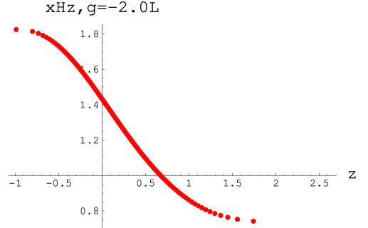
Figure 1: The scaled density $x=\rho/\rho_{c}$ as function of the redshift $z$ for the model with $\gamma=-2.0$. Note that $x$ is confined between $(x_{1},x_{2})$ (with $x_{1}(\gamma=-2.0)\simeq 1.823$ and $x_{2}(\gamma=-2.0)\simeq 0.731$) as discussed in the text.

4.2.1 Models with $\gamma\in[\ -3.34186,\ 0.141859\ ]$

Let us start our analysis considering the second region in Eq.(60). For values of $\gamma$ in this range, the term under square root in $P_{2}(x)$ and $P_{3}(x)$ gets negative values, but the right hand side is still a real quantity. To show this, let us remember the two following mathematical relations $\sqrt{b}=i\sqrt{b}$ (b real and negative), arctan${ib}=i$ arctanh${b}$ (b real), Eq.(56) may be rewritten as:

$$-3\ (1+\gamma)\ln{\left(\frac{a}{a_{0}}\right)}=\ln{P_{1}(x)}+P^{\prime}_{2}(x){\rm arctanh{P^{\prime}_{3}(x)}}$$ (61)

with :

$$P^{\prime}_{2}(x)=\frac{11\gamma-8}{\sqrt{-135\gamma^{2}-432\gamma+64}}\ ,$$ (62)

$$P^{\prime}_{3}(x)=\frac{-18\gamma x+27\gamma+8}{\sqrt{-135\gamma^{2}-432\gamma+64}}\ .$$ (63)

Eq.(61) is correctly defined for $\gamma$, in the range we are considering, provided that the logarithmic term is real. To this aim, $x$ should be in the range $]\ x_{1},\ x_{2}\ [$, being these latter the two roots of the square root term entering $P_{1}(x)$, given as :

$$x_{1,2}=\frac{8+27\gamma{\pm}\sqrt{64-432\gamma-135\gamma^{2}}}{\gamma}\ .$$ (64)

On the other hand, since $x$ is positive by its definition, we must impose the constraint $x_{1,2}\geq 0$ which means that we have to exclude all the values of $\gamma$ which lead to negative values of $x_{1}$ or $x_{2}$. This constraint allows us to narrow the second region in Eq.(60) which is now reduced to :

$$\gamma\in[\ -3.34186,\ -1\ [\ .$$ (65)

It is interesting to invert numerically Eq.(61) to get $x(z;\gamma)$, being the red-shift $z$ related to the scale factor as $a_{0}/a=1+z$. We plot the result for $\gamma=-2.0$ in Fig. 1. This plot shows some interesting features. The scaled energy density $x(z,\gamma)$ is bounded between two finite values as a consequence of the condition imposed so that the logarithmic term of Eq.(61) is correctly defined. It is interesting to observe that the model predicts that the energy density is an increasing function of time (and hence a decreasing function of red-shift as in the super-inflationary models). The two extreme values are $(x_{1},x_{2})$ that may be computed using Eq.(64) once a value of $\gamma$ in the range defined by Eq.(65) has been chosen. Furthermore, being $x$ constrained in the range $]x_{1},x_{2}[$, we also get that the model may describe the dynamics of the universe over a limited red-shift range $(z_{min},z_{max})$. This is not a serious shortcoming since the Van der Waals equation of state we are using is only an approximation (even if more realistic than the perfect fluid one) of the true unknown equation of state. It is thus not surprising that it may be applied only over a limited period of the universe evolution. It is quite easy to show (both analytically and numerically) that the lower limit of red-shift range is $z_{min}=-1$ so that the model may be used also to describe the near future evolution of universe. On the other hand, the upper limit is a function of $\gamma$, in particular, $z_{max}$ is always larger than $z\sim 12$ so that we can safely use the model to describe dynamics of the universe over the red-shift range $(z\leq 1)$ probed by SNeIa Hubble diagram. We will see, in next subsection, that the situation will be different in the other red-shift ranges defined by Eq.(60).

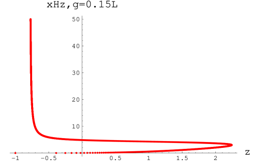
Figure 2: The scaled density $x=\rho/\rho_{c}$ as function of the redshift $z$ for the model with $\gamma=0.15$. Note that the apparent divergence on the left side is not a physical one, but only an artifact of the scale used in the plot.

4.2.2 Models with $\gamma\not\in\ [\ -3.34186,\ 0.141859\ ]$

Let us turn now to the other two ranges defined in Eq.(60). It is quite easy to show that the term under square root, entering $P_{1}(x)$ in Eq.(56), has the same sign of $\gamma$, if this parameter takes values in these regions. In order to have a positive function, we have to exclude the region $]\ -\infty,\ -3.34186\ [$ which we do not consider anymore in the following so that we can now concentrate on the range $]\ 0.141859,\ \infty\ [$.

We can further narrow it on the basis of physical considerations. To this aim, let us invert numerically Eq.(56) to get $x(z;\gamma)$. As an example, in Fig. 2 the results for $\gamma=0.15$ are sketched. This plot shows two interesting features. First, there is a limiting red-shift $z_{lim}$ such that, for $z\geq z_{lim}$, the density is not defined. This fact simply states that our model could describe the dynamical evolution of universe only for red-shifts lower than $z_{lim}$. This fact could be explained qualitatively observing that $x(z_{lim};\gamma)=3$ for every $\gamma$. For $\rho=3\rho_{c}$, we get $p\rightarrow\infty$. It is quite obvious that the universe cannot evolve until the pressure becomes finite (both positive or negative). Then, the universe starts evolving, but the density may follow two different tracks, decreasing or increasing with red-shift (that is increasing or decreasing with time). We will come back to this topic later.

We can observe that $z_{lim}$ is implicitly defined as function of $\gamma$ by the relation $x(z_{lim};\gamma)=3$ and increases with $\gamma$ faster and faster as $\gamma$ approaches the lowest value in the range we are now considering.
In the following section, we will investigate whether our model is able to reproduce the Hubble diagram of SNeIa. To this aim, the minimal request is that the model describes the dynamical evolution of matter density at least over the red-shift range probed by SNeIa, i.e. until $z\sim 0.83$. However, future observations (e.g. with the up to come SNAP satellite [47]) will be able to extend the upper limit of the range probed by SNeIa until $z\sim 1.7$. A supernova at this red-shift has been yet observed even if the estimated $z$ is very uncertain and its apparent magnitude is likely to be seriously altered by gravitational lensing effects.

Choosing a value of $\gamma$ very near to the lowest one will lead to $z_{lim}>1000$ so that our model could describe the universe from the decoupling age up to now. However, the Van der Waals equation of state is an approximation so that it should be not surprising if the model works only on a limited range for $z$. Thus, we impose an upper limit on the value of $\gamma$ by requiring that $z_{lim}(\gamma_{max})=1.7$. This leads us to the following range for $\gamma$ :

$$\gamma\ \in\ ]\ 0.141859,\ 0.152370\ [\ .$$ (66)

Before testing the models with $\gamma$ ranging in the interval defined by Eqs.(65) and (66), we come back again to Fig. 2. This plot shows that, for $\gamma\in]\ 0.141859,\ 0.152370\ [$, the universe starts evolving when $x\neq 3$, but there are two possible evolutionary tracks. From a mathematical point of view, this is a consequence of the intrinsic non linearity of Eq.(56). However, the two curves are clearly physically distinct since the density decreases or increases with the red-shift according to which track is followed. There is also another very important difference. Let us consider Eq.(14). If we ask for a today accelerating universe, we have to impose the following constraint on the present day value of the scaled density and pressure :

$$x_{0}+3y_{0}<0\ \rightarrow\ \frac{x_{0}}{8\ (3-x_{0})}\left[27\gamma x_{0}^{2}-(81\gamma+8)x_{0}+(72\gamma+24)\right]<0\ .$$

For the values of $\gamma$ in the range defined by Eq.(66), the second degree polynomial in this equation is always positive definite, so that we get an accelerating universe if :

$$3-x_{0}<0\ \longrightarrow\ x_{0}>3\ .$$

Fig. 2 shows that the evolutionary track to get a today positive value of $\ddot{a}$ is the upper one, so that we arrive to the conclusion that the accelerated models are those with an increasing density with time. Anyway, the result (from SNeIa) that the universe is now in an accelerated phase is model dependent so that, in the following, we will consider both models and test them against the observations to discriminate among the two evolutionary tracks.

4.3 The Hubble diagram of SNeIa in the Van der Waals scheme

It is well known that the use of astrophysical standard candles provides a fundamental tool to test different cosmological models. SNeIa are the best candidates to this aim since they can be accurately calibrated and can be detected at enough high red-shift. This fact allows to measure the SNeIa relation between magnitude and red-shift (i.e. the Hubble diagram) at high enough distances to discriminate among cosmological models. To this aim, one can match a given model with the observed Hubble diagram, conveniently expressed through Eq.(9), which we write as :

$$\mu(z)=5\log{d_{L}(z)}+25\ ,$$ (67)

being $\mu$ as before the distance modulus and $D_{L}(z)$ the luminosity distance calibrated with the Hubble constant. For our cosmological models, it is :

$$d_{L}(z)=\frac{c}{H_{0}}\ \sqrt{x_{0}(\gamma)}\ (1+z)\ \int_{0}^{z}{[\ \rho(z^{\prime})\ ]^{-1/2}\ dz^{\prime}}\ .$$ (68)

The distance modulus, as said, can be obtained from observations of SNeIa. The apparent magnitude $m$ at the peak is measured, while the absolute one $M$ may be deduced from template fitting or using the Multi Color Light Curve Shape method [4, 5]. The distance modulus is then $\mu=m-M$. Finally the redshift $z$ of the SNeIa is deduced from the host galaxy spectrum or (with a larger uncertainty) from the supernova spectrum directly. Our model can be fully characterized by two parameters : the today Hubble constant $H_{0}$ and the value of $\gamma$. We find their best fit values minimizing the $\chi^{2}$ defined as [46] :

$$\chi^{2}(H_{0},\gamma)=\sum_{i=1}^{N}{\frac{[\ \mu_{i}^{theor}(z;H_{0},\gamma)-\mu_{i}^{obs}\ ]^{2}}{\sigma^{2}_{\mu_{0},i}+\sigma^{2}_{mz,i}}}$$ (69)

where the sum is over the data points. In Eq.(69), $\sigma_{\mu_{0}}$ is the estimated error on the distance modulus, while $\sigma_{mz}$ is the dispersion in the distance modulus due to the uncertainty $\sigma_{z}$ on the measured red-shift. We have :

$$\sigma_{mz}=\frac{5}{\ln{10}}\left(\frac{1}{d_{L}(z)}\frac{\partial{d_{L}}}{\partial{z}}\right)\sigma_{z}\ .$$ (70)

Following Ref. [46], we assume $\sigma_{z}=200\ {\rm kms^{-1}}$ adding in quadrature $2500\ {\rm km\ s^{-1}}$ for those SNeIa whose red-shift is obtained from broad lines in their spectrum. Note that $\sigma_{mz}$ depends on the parameters we wish to determine so that we have to use an iterative procedure to minimize the $\chi^{2}$.

The the SCP [4] and HZT team [5] have detected a quite large sample of high refshift $(\simeq 0.18\div 0.83)$ SNeIa, while the Calan - Tololo survey [45] has investigated the nearby sources. Using the data in Refs. [4, 5], we have compiled a combined sample of 85 SNeIa as described in Ref. [46]. We exclude 6 likely outlier SNeIa as discussed in Ref. [4], thus ending with 79 SNeIa.

Figure 3: 1, 2 and 3 - $\sigma$ confidence regions in the $(H_{0},\gamma)$ plane for the models with $\gamma\in\ ]\ -3.34186,\ -1\ ]$.

Let us discuss first the results of the fit for the models with $\gamma\in\ [\ -3.34186,\ -1\ [$.

As we can see in Fig.3 the models fit the data quite well. This is an encouraging result which mean that the proposed equation of state leads to a magnitude - red-shift relation which is in agreement with the observed SNeIa Hubble diagram. This result is further strengthened by the estimated value of the Hubble constant. The best fit value is $H_{0}=71\ {\rm km\ s^{-1}\ Mpc^{-1}}$, while the 68$\%$ confidence range turns out to be :

$$H_{0}=(60\div 80)\ {\rm km\ s^{-1}\ Mpc^{-1}}\,,$$

which is in very good agreement with the most recent estimates in literature. For instance, the HST Key Project [49] has calibrated different local distance estimators and has found $H_{0}=72\ {\pm}\ 8\ {\rm km\ s^{-1}\ Mpc^{-1}}$.
It has to be stressed that the Hubble diagram of SNeIa (Fig.3) gives no constraint on the $\gamma$ parameter. In fact, the best fit value for this range turns out to be $\gamma=-1.03$, but the $\chi^{2}$ changes less than 1$\%$ for $\gamma$ in the range defined by Eq.(65). This is not an unexpected result since the study of density gives a density $\rho(z,\gamma)$ almost completely independent of $\gamma$ in the red-shift range probed by the available data [48].

However, the dependence on $\gamma$ becomes significative for higher red-shifts so that the prospects for using SNeIa to measure the value of $\gamma$ are quite good as soon as SNeIa at $z\simeq 1.0\div 1.7$ (a red-shift range which will be explored by the dedicated SNAP satellite) will become available [47].

Figure 4: 1, 2 and 3 - $\sigma$ confidence regions in the $(H_{0},\gamma)$ plane for the models with $\gamma\in\ ]\ 0.141859,\ 0.151237\ ]$ having the scaled energy density increasing with the 5red-shift

The results of the fit for models with $\gamma$ in the range given by Eq.(66) give also in this case that these models are able to reproduce the observed SNeIa Hubble diagram. We obtain $H_{0}=70\ {\rm km\ s^{-1}\ Mpc^{-1}}$ as best fit value for the Hubble constant, while the 68$\%$ confidence range is :

$$H_{0}=(64\div 78)\ {\rm km\ s^{-1}\ Mpc^{-1}}\,,$$

which is still in very good agreement with the most recent estimates (see Fig.4). However, the Hubble diagram of SNeIa gives no constraint on $\gamma$ parameter even for models with $\gamma$ in the range defined by Eq.(66). The best fit value turns out to be $\gamma=0.142$, but as in the previous case it is not possible to give a reliable estimate of the uncertainty on this parameter. This is again due to the almost complete degeneracy of different models for $z\leq 1$ .

On the other hand this degeneracy seems to be again eliminated using SNeIa data in the red-shift range $z\simeq 1.0\div 1.7$.

Finally, we have repeated the same analysis for models with density decreasing with time. Even if the fit is still possible, the estimated $H_{0}$ is too low, the best fit value being $40\ {\rm km\ s^{-1}\ Mpc^{-1}}$. This fact has led us to do not consider anymore this class of models thus ending with the surprising conclusion that the models which fit the data are those with the energy density increasing with time.

4.4 The age of the Universe in the Van der Waals scheme

The SNeIa–Hubble diagram fit has shown that several Van der Waals models are able to reproduce the available data giving a value of $H_{0}$ in very good agreement with the most recent estimates. Furthermore, the matching with the data has allowed to reject models with $\rho$ decreasing with time so that we do not consider them anymore in the following analysis. However, we are still not able to constrain the value of $\gamma$. To this aim, we can use the available estimates of the age of the universe. As a first step, we have to determine how the scale factor $a$ depends on the time $t$. From Eq.(16) and the choice (53), we get :

$$t-t_{lim}=\frac{\sqrt{x_{0}(\gamma)}}{H_{0}}\int_{a_{lim}}^{a}{[\ a^{\prime}\sqrt{x(a^{\prime})}\ ]^{-1}\ da^{\prime}}\,,$$ (71)

where $a_{lim}$ is the value of $a$ for the upper limit of red-shift range where the model may describe the evolution of the universe and $t_{lim}$ is the corresponding time. We have also imposed $a_{0}=1$ for the sake of shortness. This relation cannot be analytically inverted, but it is quite easy to invert numerically. Imposing $a=1$ in Eq.(71), we have an estimate of $t_{0}-t_{lim}$, but we do not know the value of $t_{lim}$, i.e. the age of the universe at a red-shift when the model starts to describe the dynamical evolution. On the other hand, we can evaluate the quantity :

$$t_{0}-t_{ref}=\frac{\sqrt{x_{0}(\gamma)}}{H_{0}}\int_{a_{ref}}^{1}{[\ a^{\prime}\sqrt{x(a^{\prime})}\ ]^{-1}\ da^{\prime}}\,,$$ (72)

being $t_{ref}$ the age of the universe at a given red-shift $z_{ref}$ with $a_{ref}=a(z_{ref})$. This approach allows to constrain the values of $\gamma$, even if we do not know $t_{lim}$, provided that we have an independent estimate of $t_{ref}$. To this aim, we can use the age of an early-type high red-shift galaxy which can be estimated in a way which does not depend on the background cosmological model, but only on astrophysical assumptions on the galaxy formation scenario and stellar evolution. As a reference value, we use :

$$z_{ref}=1.55\ ,\ t_{ref}=t_{1.55}>3.5\ {\rm Gyr}$$

as first estimated in [50] for the radio galaxy 53W091 [51]. Different estimates of $t_{0}$ are present in literature. Recent determinations of $t_{0}$ from the age of globular clusters give $t_{0}=11.5\ {\pm}\ 1.5$ Gyr [52, 53], while the analysis of the SNeIa Hubble diagram suggests $t_{0}=14.9$ (for $H_{0}=63km\,s^{-1},Mpc^{-1}$) [4]. A multivariate analysis of combined BOOMERanG, DASI and MAXIMA data on the CMBR anisotropy spectrum gives estimates of $t_{0}$ ranging from $\sim 13$ to $\sim 16$ Gyr according to the former ones used in the maximum likelihood estimation of the parameters [54]. We use $t_{0}=10\div 16$ Gyr so we get :

$$t_{0}-t_{1.55}=6.5\div 12.5\ {\rm Gyr}$$ (73)

as a conservative limit on this quantity.

For each value of $\gamma$ in the range defined by Eqs.(65) and (66) and for $H_{0}$ in the corresponding 1 $\sigma$ confidence interval, we can determine the estimated range for $t_{0}-t_{1.55}$. Imposing that this range is contained within the range given by Eq.(73), we find the constraint :

$$\gamma\ \in\ [\ -1.95,\ -1.40\ ]\$$ (74)

which we consider as our final estimate of the physically acceptable range for $\gamma$. Note that the range in Eq.(66) is completely cut out by this constraint since the predicted values of $t_{0}-t_{1.55}$ are much higher than the (quite conservative) limits we have imposed.

4.5 Discussion of results in Van der Waals cosmology

We have investigated the possibility that a cosmological model with a Van der Waals equation of state can give account of the accelerating expansion of the universe as suggested by the SNeIa data.

As a first step, starting from mathematical and physical considerations, we have constrained the effective parameter $\gamma$ of the model to take values in the range $[\ -3.14186,\ -1\ [$ $\ \cup\ ]\ 0.141859,\ 0.15237\ ]$. In these regions, the matter energy density can be both increasing or decreasing with time as showed in Figs. 1 and 2 and the quantity $x+3y$ results always negative which is consistent with an accelerated phase of the universe evolution.

As a following step, we have fitted these models with the data of SNeIa-Hubble diagram. The fitting procedure has lead us to conclude that both the intervals of $\gamma$ are physically significative, but the decreasing behaviour of energy density in the range $]0.141859,0.15237]$ has to be discarded since the estimated Hubble constant is only $40\ {\rm km\ s^{-1}\ Mpc^{-1}}$, in strong disagreement with results in literature. On the other hand, the best fit values of the parameters turn out to be :

$$\gamma=-1.09\ ,\ H_{0}=71\ {\rm km\ s^{-1}\ Mpc^{-1}}\ ,$$

for models with $\gamma\in\ ]\ -3.34186,\ -1\ [$ and :

$$\gamma=0.142\ ,\ H_{0}=70\ {\rm km\ s^{-1}\ Mpc^{-1}},$$

for models with $\gamma\in\ ]\ 0.14186,\ 0.15237\ [$ and the energy density increasing with time. The results for $H_{0}$ are in perfect agreement with the estimates obtained with different methods such as the calibration of local distance estimators [49], which is an evidence of the validity of our models. Unfortunately, the very small variation of the energy density with $\gamma$ in the red-shift range probed by available data does not let us to discriminate in a useful way between different values of this parameter. However, higher red-shift SNeIa data (as the ones that will be collected by the next to come SNAP satellite) will be able to break the degeneracy among the different values of $\gamma$ since they will probe a red-shift region where the energy density is more sensitive to the effective parameter of the theory.

As a possible test to break the degeneracy among the values of $\gamma$ with nowaday available data, we have estimated the quantity $t_{0}-t_{1.55}$, being $t_{0}$ the nowaday age of the universe and $t_{1.55}=t(z=1.55)$. For a fixed $\gamma$, we estimate a range for $t_{0}-t_{1.55}$ changing $H_{0}$ in the corresponding 68 $\%$ confidence region and compare it with the conservative limit given in Eq.(73). This test allows us to exclude the range in Eq.(66) since the predicted values of $t_{0}-t_{1.55}$ are much higher than 12.5 Gyr so that we turn out with a final estimate for $\gamma$ as :

$$\gamma\ \in\ [\ -1.95,\ -1.40\ ]\ .$$

The analysis presented suggests that a cosmological model characterized by a Van der Waals equation of state is a novel and interesting approach to explain the accelerating expansion of the universe. Indeed, for values of $\gamma$ in the range given by Eq.(74), the models are able to fit quite well the SNeIa Hubble diagram and predict an age of the universe consistent with recent estimates obtained with completely different methods. Another feature of the selected models is the behaviour of the energy density which is an increasing function of time (i.e. decreasing with $z$ as shown in Fig. 1) bounded between two finite values. However, some models of super - inflation also predict such a behaviour so that it should be interesting to see whether a cosmological fluid with a Van der Waals equation of state could be accomodated within the framework of these theories.

5 Second hypothesis: Curvature Quintessence

5.1 The model

There is no a priori reason to restrict the gravitational Lagrangian to a linear function of Ricci scalar $R$ minimally coupled with matter [55]. Furthermore, we have to note that, recently, some authors have taken into serious consideration the idea that there are no ”exact” laws of physics, but that Lagrangians of physical interactions are ”stochastic” functions with the property that local gauge invariances (i.e. conservation laws) are well approximated in the low energy limit with the properties that fundamental physical constants can vary [56]. This scheme was adopted in order to treat the quantization on curved spacetimes. The result was that either interactions among quantum fields and background geometry or the gravitational self–interactions yield corrective terms in the Einstein–Hilbert Lagrangian [57]. Futhermore, it has been realized that such corrective terms are inescapable if we want to obtain the effective action of quantum gravity on scales closed to the Planck length [58]. They are higher–order terms in curvature invariants as $R^{2}$, $R^{\mu\nu}R_{\mu\nu}$, $R^{\mu\nu\alpha\beta}R_{\mu\nu\alpha\beta}$, $R\Box R$, or $R\Box^{k}R$, or nonminimally coupled terms between scalar fields and geometry as $\phi^{2}R$. Terms of this kind arise also in the effective Lagrangian of strings and Kaluza–Klein theories when the mechanism of dimensional reduction is working [59].

Besides fundamental physics motivations, all these theories have acquired a huge interest in cosmology due to the fact that they ”naturally” exhibit inflationary behaviours and that the related cosmological models seem very realistic [60, 61]. Furthermore, it is possible to show that, via conformal transformations, the higher–order and nonminimally coupled terms (Jordan frame) always corresponds to the Einstein gravity plus one or more than one minimally coupled scalar fields (Einstein frame) [62, 63, 64, 65, 66] so that these geometric contributions can always have a ”matter-like” interpretation.
Here we want to investigate the possibility that quintessence could be achieved by extra-curvature contributions. We focus our attention on fourth-order theories of gravity [67].
A generic fourth–order theory in four dimensions can be described by the action

$${\cal A}=\int d^{4}x\sqrt{-g}\left[f(R)+{L}_{M}\right]\,{,}$$ (75)

where $f(R)$ is a function of Ricci scalar $R$ and ${L}_{M}$ is the standard matter Lagrangian density. We are using physical units $8\pi G_{N}=c=\hbar=1$. The field equations are

$$f^{\prime}(R)R_{\alpha\beta}-\frac{1}{2}f(R)g_{\alpha\beta}=f^{\prime}(R)^{;\alpha\beta}(g_{\alpha\mu}g_{\beta\nu}-g_{\alpha\beta}g_{\mu\nu})+\tilde{T}^{M}_{\alpha\beta}\,,$$ (76)

which can be recast in the more expressive form

$$G_{\alpha\beta}=R_{\alpha\beta}-\frac{1}{2}g_{\alpha\beta}R=T^{curv}_{\alpha\beta}+T^{M}_{\alpha\beta}\,,$$ (77)

where

$$T^{curv}_{\alpha\beta}=\frac{1}{f^{\prime}(R)}\left\{\frac{1}{2}g_{\alpha\beta}\left[f(R)-Rf^{\prime}(R)\right]+f^{\prime}(R)^{;\alpha\beta}(g_{\alpha\mu}g_{\beta\nu}-g_{\alpha\beta}g_{\mu\nu})\right\}$$ (78)

and

$$T^{M}_{\alpha\beta}=\frac{1}{f^{\prime}(R)}\tilde{T}^{M}_{\alpha\beta}\,,$$ (79)

is the stress-energy tensor of matter where we have taken into account the nonmnimal coupling to geometry. The prime indicates the derivative with respect to $R$. If $f(R)=R+2\Lambda$, the standard second–order gravity is recovered.
It is possible to reduce the action to a point-like, FRW one. We have to write

$${\cal A}_{curv}=\int dt{\cal L}(a,\dot{a};R,\dot{R})\,{,}$$ (80)

where dot indicates derivative with respect to the cosmic time. The scale factor $a$ and the Ricci scalar $R$ are the canonical variables. This position could seem arbitrary since $R$ depends on $a,\dot{a},\ddot{a}$, but it is generally used in canonical quantization [68, 69, 70]. The definition of $R$ in terms of $a,\dot{a},\ddot{a}$ introduces a constraint which eliminates second and higher order derivatives in action (80), and gives a system of second order differential equations in $\{a,R\}$. Action (80) can be written as

$${\cal A}_{curv}=2\pi^{2}\int dt\left\{a^{3}f(R)-\lambda\left[R+6\left(\frac{\ddot{a}}{a}+\frac{\dot{a}^{2}}{a^{2}}+\frac{k}{a^{2}}\right)\right]\right\}\,{,}$$ (81)

where the Lagrange multiplier $\lambda$ is derived by varying with respect to $R$. It is

$$\lambda=a^{3}f^{\prime}(R)\,{.}$$ (82)

The point-like Lagrangian is then

$${\cal L}={\cal L}_{curv}+{\cal L}_{M}=a^{3}\left[f(R)-Rf^{\prime}(R)\right]+6a\dot{a}^{2}f^{\prime}(R)+$$

$$\qquad+6a^{2}\dot{a}\dot{R}f^{\prime\prime}(R)-6kaf^{\prime}(R)+a^{3}p_{M}\,,$$ (83)

where we have taken into account also the fluid matter contribution which is, essentially, a pressure term [71].

The Euler-Lagrange equations are

$$2\left(\frac{\ddot{a}}{a}\right)+\left(\frac{\dot{a}}{a}\right)^{2}+\frac{k}{a^{2}}=-p_{tot}\,,$$ (84)

and

$$f^{\prime\prime}(R)\left[R+6\left(\frac{\ddot{a}}{a}+\frac{\dot{a}^{2}}{a}^{2}+\frac{k}{a^{2}}\right)\right]=0\,.$$ (85)

The dynamical system is completed by the energy condition

$$\left(\frac{\dot{a}}{a}\right)^{2}+\frac{k}{a^{2}}=\frac{1}{3}\rho_{tot}\,.$$ (86)

Combining Eq.(84) and Eq.(86), we obtain

$$\left(\frac{\ddot{a}}{a}\right)=-\frac{1}{6}\left[\rho_{tot}+3p_{tot}\right]\,,$$ (87)

where it is clear that the accelerated or decelerated behaviour depends on the r.h.s. How it is evident equations (84)-(87) generalize in a very simply way the system (14)-(16) for standard cosmological model.
Now it holds:

$$p_{tot}=p_{curv}+p_{M}\;\;\;\;\;\rho_{tot}=\rho_{curv}+\rho_{M}\,,$$ (88)

where we have distinguished the curvature and matter contributions.

In fact by curvature-stress-energy tensor, we can define a curvature pressure

$$p_{curv}=\frac{1}{f^{\prime}(R)}\left\{2\left(\frac{\dot{a}}{a}\right)\dot{R}f^{\prime\prime}(R)+\ddot{R}f^{\prime\prime}(R)+\dot{R}^{2}f^{\prime\prime\prime}(R)-\frac{1}{2}\left[f(R)-Rf^{\prime}(R)\right]\right\}\,,$$ (89)

and a curvature density

$$\rho_{curv}=\frac{1}{f^{\prime}(R)}\left\{\frac{1}{2}\left[f(R)-Rf^{\prime}(R)\right]-3\left(\frac{\dot{a}}{a}\right)\dot{R}f^{\prime\prime}(R)\right\}\,.$$ (90)

From Eq.(87), the accelerated behaviour is achieved if

$$\rho_{tot}+3p_{tot}<0\,,$$ (91)

which means

$$\rho_{curv}>\frac{1}{3}\rho_{tot}\,,$$ (92)

assuming that all matter components have non-negative pressure.

In other words, conditions to obtain acceleration depends on the relation

$$\rho_{curv}+3p_{curv}=\frac{3}{f^{\prime}(R)}\left\{\dot{R}^{2}f^{\prime\prime\prime}(R)+\left(\frac{\dot{a}}{a}\right)\dot{R}f^{\prime\prime}(R)+\ddot{R}f^{\prime\prime}(R)-\frac{1}{3}\left[f(R)-Rf^{\prime}(R)\right]\right\}\,,$$ (93)

which has to be compared with matter contribution. However, it has to be

$$\frac{p_{(curv)}}{\rho_{curv}}=\gamma_{curv}\,,\qquad-1\leq\gamma_{curv}<0\,.$$ (94)

The form of $f(R)$ is the main ingredient to obtain this curvature quintessence. As simple choice in order to fit the above prescriptions, we ask for solutions of the form

$$f(R)=f_{0}R^{n}\,,\qquad a(t)=a_{0}\left(\frac{t}{t_{0}}\right)^{\alpha}\,.$$ (95)

The interesting cases are for $n\neq 1$ (being $n=1$ Einstein gravity) and $\alpha\geq 1$ (accelerated behaviour). Inserting Eqs.(95) into the above dynamical system, we obtain the exact solutions

$$\alpha=2\,;\qquad n=-1,3/2\,;\qquad k=0\,.$$ (96)

In both cases, the deceleration parameter is

$$q_{0}=-\frac{1}{2}\,,$$ (97)

in perfect agreement with the observational results.

The case $n=3/2$ deserves further discussion. It is interesting in conformal transformations from Jordan frame to Einstein frame [72, 73] since it is possible to give explicit form of scalar field potential. In fact, if

$$\tilde{g}_{\alpha\beta}\equiv f^{\prime}(R)g_{\alpha\beta}\,{,}\qquad\varphi=\sqrt{\frac{3}{2}}\ln f^{\prime}(R)\,{,}$$ (98)

we have the conformal equivalence of the Lagrangians

$${\cal L}=\sqrt{-g}\,f_{0}R^{3/2}\longleftrightarrow\tilde{{\cal L}}=\sqrt{-\tilde{g}}\left[-\frac{\tilde{R}}{2}+\frac{1}{2}\nabla_{\mu}\varphi\nabla^{\mu}\varphi-V_{0}\exp\left(\sqrt{\frac{2}{3}}\varphi\right)\right]\,,$$ (99)

in our physical units. This is the so–called Liouville field theory and it is one of the few cases where a fourth–order Lagrangian can be expressed, in the Einstein frame, in terms of elementary functions under a conformal transformation. Furthermore this is a case in which quintessence can be achieved also by an exponential potential.
It is possible to obtain the general solution [74]

$$a(t)=a_{0}[c_{4}t^{4}+c_{3}t^{3}+c_{2}t^{2}+c_{1}t+c_{0}]^{1/2}\,{.}$$ (100)

The constants $c_{i}$ are combinations of the initial conditions. Their particular values determine the type of cosmological evolution. For example, $c_{4}\neq 0$ gives a power law inflation while, if the regime is dominated by the linear term in $c_{1}$, we get a radiation–dominated stage.
These cases belong to an entire family of exact solutions for the quintessence curvature model. In fact solving Eqs. (87) and (88) in the limit in which matter can be neglected (this hypothesis can be considered well posed in a toy model) and assuming for $f(R)$ and $a(t)$ behaviours like (95), we obtain the algebraic system for the parameters $n$ and $\alpha$

$$\left\{\begin{array}[]{ll}\alpha[\alpha(n-2)+2n^{2}-3n+1]=0\\ \\ \alpha[n^{2}+\alpha(n-2-n-1)]=n(n-1)(2n-1)\\ \end{array}\right.$$ (101)

from which we have the solutions:

$$\begin{array}[]{cc}\alpha=0\longrightarrow n=0,\,1/2,\,1\\ \\ \alpha=\displaystyle\frac{-2n^{2}+3n-1}{n-2}\,,\qquad n\,\,.\end{array}$$ (102)

The cases for $\alpha=0$ give static models not interesting to discuss. The cases for $\alpha$ and $n$ generic deserve more attention since a class of cosmological quintessential behaviours can be found. In Fig.5 there is a sketch of the situation.

Figure 5: The plot shows the behaviour of $\alpha$ and against $n$. It is evident a region in which the power law of the scale factor is more than one and correspondently the parameter $\gamma_{(curv)}$ of state equation is negative .

The state equation for the class of solutions $n$ and $\alpha=\displaystyle{\frac{-2n^{2}+3n-1}{n-2}}$ gives

$$\gamma_{curv}=-\frac{6n^{2}-7n-1}{6n^{2}-9n+3}\,\,.$$ (103)

Accelerated behaviours for increasing scale factors are possible only for $\gamma_{curv}<0$ how requested for a cosmological fluid with negative pressure. The whole approach seems intriguing in relation to the possibility to get an accelerated phase of universe expansion as an effect of a higher-order curvature Lagrangian.

At this point, to obtain constraints on $n$ and to match with the observations we take into account data, in particular we compare this model in relation to SNeIa results as yet done for the Van der Waals case in ([48] and [75]). To complete our analysis we have to evaluate also the age prediction of curvature quintessence model as a function of the parameter $n$.
In this sense, some results are present in literature where the form of $f(R)$ is selected by the CMBR constraint [76].

5.2 Matching Curvature Quintessence with observations

5.2.1 SNeIa matching

In order to verify if such an approach has real perspective to be physically acceptable, we match the theory with observational data. In this way, we can constraint the parameters.
To this aim we consider the supernovae observations, in particular we use the data in [4, 5] as in the Van der Waals case.
Starting from these data, it is possible to perform a comparison between the theoretically predicted expression of distance modulus and its observational value. In this case the luminosity distance can be expressed by the general expression:

$$d_{L}=\frac{c}{H_{0}}(1+z)\int_{0}^{z}{\frac{1}{E_{(}{\zeta})}}d{\zeta}$$ (104)

where $E(\zeta)=\displaystyle\frac{H_{0}}{H}$ and $c$ is the light speed having reintroduced the standard units.
Starting from Eq. (95), the Hubble parameter, in terms of redshift, is given by the relation

$$H(z)=H_{0}(1+z)^{1/{\alpha}}$$ (105)

where $\alpha$ is given in (102) as a function of $n$.
The luminosity distance is now:

$$d_{L}(z,H_{0},n)=\frac{c}{H_{0}}(1+z)\int_{0}^{z}(1+\zeta)^{-1/\alpha}d{\zeta}$$ (106)

and after the integration, we obtain

$$d_{L}(z,H_{0},n)=\frac{c}{H_{0}}\left(\frac{\alpha}{\alpha-1}\right)(1+z)\left[(1+z)^{\frac{\alpha}{\alpha-1}}-1\right]\,.$$ (107)

This expression is not defined for $\alpha=0,1$, so we have to check the luminosity distance taking into account the existence of such singularities. As a consequence the fit can be performed in five intervals of $n$, that is: $n<\displaystyle\frac{1}{2}(1-\sqrt{3})\,,\,\ \frac{1}{2}(1-\sqrt{3})<n<\frac{1}{2}\,,\,\ \frac{1}{2}<n<1\,,1<n<\frac{1}{2}(1+\sqrt{3})\,,\,\ n>\frac{1}{2}(1+\sqrt{3})$.
Hubble parameter, as a function of $n$, shows the same trend of $\alpha$ (Fig.5). We find that for $n$ negative, lower than -100, it is strictly increasing while for $n$ positive, greater than 100, it is strictly decreasing. In relation to this feature, we have tested $n$ for values ranging in these limits because, as we shall see below, outside of this range the value of the age of universe becomes manifestly not physically significant. The results can be showed in the Table 1. From Table 1, in relation to the best fit values of $H_{0}$ and $\chi^{2}$, we can only exclude the range $\displaystyle\frac{1}{2}<n<1$ as physically not interesting. In the other cases, the results give interesting best fit values both for the Hubble parameter and the $\chi^{2}$, indicating that such a model could represent a significant theoretical background to explain SNeIa data.

Range	$H_{0}^{best}$($km\,sec^{-1}Mpc^{-1}$)	$n^{best}$	$\chi^{2}$
$-100<n<1/2(1-\sqrt{3})$	$65$	$-0.73$	$1.003$
$1/2(1-\sqrt{3})<n<1/2$	$63$	$-0.36$	$1.160$
$1/2<n<1$	$100$	$0.78$	$348.97$
$1<n<1/2(1+\sqrt{3})$	$62$	$1.36$	$1.182$
$1/2(1+\sqrt{3})<n<3$	$65$	$1.45$	$1.003$
$3<n<100$	$70$	$100$	$1.418$

Table 1: Results obtained fitting the curvature quintessence model with SnIa data. First column indicate the range of $n$ studied, column two gives the relative best fit $H_{0}$, column three $n^{best}$, column four the $\chi^{2}$ index.

We have to note that the best fit is completely degenerate with respect to the $n$ parameter. This peculiarity indicates that $\chi^{2}$ varies slightly with respect to $n$ hindering the possibilities of constrain $n$.

5.2.2 The age of universe in Curvature Quintessence approach

The age of the universe can be simply obtained from a theoretical point of view if one has the value of the Hubble parameter. Now, in curvature quintessence model from the definition of $H$, using the relation (95), we have:

$$t=\alpha H^{-1}$$ (108)

which from $\alpha$ (102) becomes

$$t=\frac{-2n^{2}+3n-1}{n-2}H^{-1},$$ (109)

so, the today value of the age of universe simply is $t=\alpha(n)H_{0}^{-1}$

By a simple algorithm we can evaluate the age of universe taking into account both the intervals and the $1\sigma$ range of variability of the Hubble parameter, deduced from the supernovae fit for each interval. We have considered as good predictions, age estimates included between 10 and 18 Gyr.
First of all we have discarded the intervals of $n$ which give a negative value of $t$. Obviously from Eq.(108), negative values for the age of the universe are obtained for negative values of $\alpha$, so we have to exclude the ranges $1/2<n<1$ and $n>2$ (Fig.5). The results are shown in Table 2.

Range	$\Delta H(km\,sec^{-1}Mpc^{-1})$	$\Delta{n}$	$t(n^{best})(Gyr)$
$-100<n<1/2(1-\sqrt{3})$	$50-80$	$-0.67\leq n<-0.37$	$23.4$
$1/2(1-\sqrt{3})<n<1/2$	$57-69$	$-0.37<n\leq-0.07$	$15.6$
$1<n<1/2(1+\sqrt{3})$	$56-70$	$1.28\leq n<1.36$	$15.3$
$1/2(1+\sqrt{3})<n<2$	$54-78$	$1.37<n\leq 1.43$	$24.6$

Table 2: The results of the age test. In the first column is presented the tested range. Second column shows the $1\sigma$ $H_{0}$ range obtained by supernovae test, while in the third we give the $n$ intervals, that is the values of $n$ which allow to obtain ages of the universe comprised between 10 and 18 $Gyr$. In the last column, the values of the age obtained for the best fit value of each interval are reported.

As we have said above this test gives interesting results.
The last check for our model is to verify if the range of $n$ significant for the data provides also an accelerated rate of expansion. This test can be easily performed starting by relations (4), (95) and (102). To have an accelerated behaviour, the scale factor function $a=a_{0}t^{\alpha}$ has to get values of $\alpha$ negative or positive greater than one. We obtain that intervals $-0.67\leq n\leq 0.37$ and $1.37\leq n\leq 1.43$ provide a negative deceleration parameter with $\alpha>1$, that is cosmological models expanding with an accelerated rate. Conversely the other two intervals of Table 2 do not give interesting cosmological dynamics in this sense ($q_{0}>0,0<\alpha<1$).
Finally we are able to state that cosmological models based on a relativistic lagrangian with a generic power of $R$ (different from one) are physically coherent with observations.
This results indicate again that quintessence can be achieved without scalar fields starting from effective fundamental theories.

6 Third hypothesis: Torsion quintessence

6.1 The model

Taking into account torsion is a straightforward generalization to implement concepts as spin in General Relativity [77, 78]. However, it was soon evident that torsion, as considered e.g. in Einstein-Cartan-Sciama-Kibble (ECKS) theory, does not seems to give relevant effects in the observed astrophysical structures. Nevertheless it was found that for densities of the order of $10^{47}g/cm^{3}$ for electrons and $10^{54}g/cm^{3}$ for protons and neutrons, torsion could give observable consequences if all the spins of the particles are aligned. These huge densities can be reached only in the early universe so that cosmology is the only viable approach to test torsion effects [79]. However no relevant tests confirming the presence of torsion have been found until now and it is still an open debate if the space-time is Riemannian or not. Considering the cosmological point of view and, in particular the primordial phase transitions and inflation [1, 2, 80], it seems very likely that, in some regions of the early universe, the presence of local magnetic fields could have aligned the spins of particles. At very high densities, this effect could influence the evolution of primordial perturbations remaining as an imprint in today observed large scale structures. In other words, a main goal could be to select perturbation scales connected to the presence of torsion in early epochs which give today-observable cosmological effects [81].

From another point of view, the presence of torsion could give observable effects without taking into account clustered matter. Here, we want to investigate if the quintessential scheme can be achieved by taking into account theories of gravity with torsion [82].

In the ECSK theory, the affine connection is non-symmetric in its lower indices and the antisymmetric part

$$\Gamma^{a}_{[bc]}=S^{\phantom{bc}a}_{bc}$$ (110)

is called torsion. Usually, we can divide such an antisymmetric part into three components: one of them is irreducible, while the other two can be set to zero [83, 85]. This assumption yields the simplest theory containing torsion.

Furthermore, we can express by a 4-vector

$$\sigma^{a}=\epsilon^{abcd}S_{bcd}$$ (111)

the totally antisymmetric part of torsion. If one imposes to it the symmetries of a background which is homogeneous and isotropic, it follows that, in comoving coordinates, only the component $\sigma^{0}$ survives as a function depending only on cosmic time (see [83, 85, 86]).

For a perfect fluid, the Einstein-Friedmann cosmological equations in presence of torsion can be written as usual

$$\frac{\ddot{a}}{a}=-\frac{1}{6}(\tilde{\rho}+3\tilde{p})\,,$$ (112)

and

$$\left(\frac{\dot{a}}{a}\right)^{2}+\frac{k}{a^{2}}=\frac{1}{3}\tilde{\rho}\,.$$ (113)

Energy density and pressure can be assumed in the forms [83, 85]

$$\tilde{\rho}=\rho+f^{2}\,,\qquad\tilde{p}=p-f^{2}\,,$$ (114)

where $f$ is a function related to $\sigma^{0}$, while $\rho$ and $p$ are the usual quantities of General Relativity. This choice can be pursued since we can define $S_{abc}=S_{[abc]}=f(t)$ where $f(t)$ is a generic function of time which we consider as the source of torsion. For a detailed discussion of this point see [85].

As usual, we can define a stress-energy tensor of the form

$$T^{tot}_{ab}=(\tilde{p}+\tilde{\rho})u_{a}u_{b}-\tilde{p}g_{ab}\,,$$ (115)

which, by Eqs. (114), can be splitted as

$$T^{tot}_{ab}=T^{M}_{ab}+T^{torsion}_{ab}\,.$$ (116)

Due to the contracted Bianchi identity, we have

$$T^{tot\,;b}_{ab}=0\;;$$ (117)

from which, we can assume that (cfr. [84])

$$T^{M;b}_{ab}=0\,,\qquad T^{torsion\,;b}_{ab}=0\,.$$ (118)

In the FRW space-time, Eq.(117) becomes

$$\dot{\tilde{\rho}}+3H(\tilde{\rho}+\tilde{p})=0$$ (119)

which is

$$\dot{\rho}+3H(\rho+p)=-2f\dot{f}\,.$$ (120)

From Eqs.(118), both sides of (120) vanish independently so that

$$f(t)=f_{0}=\mbox{constant.}$$ (121)

In other worlds, a torsion field gives rise to a constant energy density, i.e. a ${\it torsion}-\Lambda$ term. Taking into account standard matter which equation of state is defined into the above Zeldovich range, we obtain

$$\tilde{\rho}=\rho_{0}\left[\frac{a_{0}}{a}\right]^{3(\gamma+1)}+f_{0}^{2}\,.$$ (122)

Inserting this result into the cosmological equations, we get, in any case, a monotonic expansion being $f_{0}^{2}>0$, $\dot{a}^{2}>0$. The condition to obtain the accelerated behaviour is

$$\rho+3p<2f_{0}^{2}\,,$$ (123)

so that acceleration depends on the torsion density.

In a dust-dominated universe, we have

$$\tilde{\rho}=\rho_{0}\left(\frac{a_{0}}{a}\right)^{3}+f_{0}^{2}\,,\qquad\tilde{p}=-f_{0}^{2}\,,$$ (124)

and then solving the cosmological equations we obtain the general solution:

$$a(t)=\left(\frac{a_{0}^{3}\rho_{0}}{2f_{0}}\right)^{1/3}\left[\cosh(f_{0}t)-1\right]^{1/3}\,.$$ (125)

Obviously, if $f_{0}t\rightarrow 0$, we have $\displaystyle{\cosh(f_{0}t)-1\simeq(f_{0}t)^{2}}$ and then $a\sim t^{2/3}$, as it has to be.

This results tell us that a sort of dark energy (a torsion-$\Lambda$ term) can be obtained without considering additional scalar fields in the dynamics but only assuming that the space-time is $U_{4}$ instead of $V_{4}$. A preminent role is played by the type of torsion we are going to consider [85]. However, such a density should be comparable to the observed limits of dark energy (i.e. $\Omega_{\Lambda}\sim 0.65\div 0.7$) in order to give relevant effects. Another point is that such a torsion quintessence should match the issues of cosmic coincidence [11] as scalar field quintessence. This point strictly depends on the type of torsion since torsion can be or not related to the spin density [85]. In the first case, the spin of baryonic and non-baryonic matter would rule the dark energy (torsion) density.

6.2 Matching Torsion quintessence with observations

6.2.1 The Supernovae SNe Ia method

As in previous cases we compare the theoretical estimates of luminosity distance with the results obtained for type Ia supernovae. Our analysis is based again on the sample data [46] from SCP and HZT observations [4, 5]

The luminosity distance in the model we are considering is completely equivalent to the one in a spatially flat universe with a non-zero cosmological constant. Thus $d_{L}(z)$ is simply given as :

$$d_{L}(z)=(1+z)\int_{0}^{z}{dz^{\prime}[\Omega_{M}(1+z^{\prime})^{3}+\Omega_{tor}]^{-1/2}}\ .$$ (126)

where $\Omega_{tor}=1-\Omega_{M}$ plays the same role as the usual $\Omega_{\Lambda}$.

Our model can be, so, fully characterized by two parameters : the today Hubble constant $H_{0}$ and the matter density $\Omega_{M}$. We find their best fit values minimizing the $\chi^{2}$ defined in this case as :

$$\chi^{2}(H_{0},\Omega_{M})=\sum_{i}{\frac{[\mu_{i}^{theor}(z_{i}|H_{0},\Omega_{M})-\mu_{i}^{obs}]^{2}}{\sigma_{\mu_{0},i}^{2}+\sigma_{mz,i}^{2}}}$$ (127)

where the sum is over the data points [46].
We remember that the $\sigma_{\mu_{0}}$ and $\sigma_{m_{z}}$ are the errors related to the distance modulus evaluation, their estimate is done as in the previous cases [46].
The results of the fit are presented in Fig.6 where we show the 1,2 and 3 $\sigma$ confidence regions in the $(\Omega_{M},H_{0})$ plane.

Figure 6: 1, 2 and 3$\sigma$ confidence regions in the $(\Omega_{M},H_{0})$ plane. The central dot represents the best fit values : $\Omega_{M}=0.3,H_{0}=65.4\ {\rm km\ s^{-1}\ Mpc^{-1}}$ ,

The best fit values (with $1\sigma$ error) turn out to be :

$$\Omega_{M}=0.30\pm 0.08\ \ ,\ \ H_{0}=65.4\pm 1.2\ km\ s^{-1}\ Mpc^{-1}\ .$$

which allow to conclude that a torsion $\Lambda$-term could explain observation very well. On the other hand, we can estimate the torsion density contributions which result to be :

$$f_{0}^{2}=(5.6\pm 0.7){\times}10^{-30}\ g\ cm^{-3}\,,$$

which is a good value if compared to the cosmological critical density. It is worthwhile to note that, in the case of SNeIa, the error on $H_{0}$ does not take into account systematic uncertainties due to possible calibration errors.

6.2.2 The Sunyaev-Zeldovich/X-ray method

Besides the above results, we can discuss how the Hubble constant $H_{0}$ and the torsion density parameter $\Omega_{\it tor}$ can be constrained also by the angular diameter distance $D_{A}$ as measured using the Sunyaev-Zeldovich effect (SZE) and the thermal bremsstrahlung (X-ray brightness data) for galaxy clusters.
We will limit our analysis to the so called thermal or static SZE, which is present in all the clusters, neglecting the ${\it kinematic}$ effect, which is present in those clusters with a nonzero peculiar velocity with respect to the Hubble flow along the line of sight. Typically the thermal SZE is an order of magnitude larger than the kinematic one. The shift of temperature is:

$$\frac{\Delta T}{T_{0}}=y\left[x\,\mbox{coth}\,\left(\frac{x}{2}\right)-4\right],$$ (128)

where ${\displaystyle x=\frac{h\nu}{k_{B}T}}$ is a dimensionless variable, $T$ is the radiation temperature, and $y$ is the so called Compton parameter, defined as the optical depth $\tau=\sigma_{T}\int n_{e}dl$ times the energy gain per scattering:

$$y=\int\frac{K_{B}T_{e}}{m_{e}c^{2}}n_{e}\sigma_{T}dl.$$ (129)

In Eq. (129), $T_{e}$ is the temperature of the electrons in the intracluster gas, $m_{e}$ is the electron mass, $n_{e}$ is the numerical density of electrons, and $\sigma_{T}$ is the cross section of Thompson electron scattering. We have used the condition $T_{e}\gg T$ ($T_{e}$ is of the order $10^{7}\,K$ and $T$, which is the CMBR temperature is $\simeq 2.7K$). Considering the low frequency regime of the Rayleigh-Jeans approximation, we obtain

$$\frac{\Delta T_{RJ}}{T_{0}}\simeq-2y$$ (130)

The next step to quantify the SZE decrement is that we need to specify the models for the intracluster electron density and temperature distribution. The most commonly used model is the so called isothermal $\beta$ model [87]. We have

$$n_{e}(r)=n_{e}(r)=n_{e_{0}}\left(1+\left(\frac{r}{r_{e}}\right)^{2}\right)^{-\frac{3\beta}{2}}\,,$$ (131)

$$T_{e}(r)=T_{e_{0}}~{},$$ (132)

being $n_{e_{0}}$ and $T_{e_{0}}$, respectively the central electron number density and temperature of the intracluster electron gas, $r_{e}$ and $\beta$ are fitting parameters connected with the model [88]. For the effect of cluster modelling see [89]. From Eq. (129) we have

$$\frac{\Delta T}{T_{0}}=-\left(\frac{2K_{B}\sigma_{T}T_{e_{0}}\,n_{e_{0}}}{m_{e}c^{2}}\right)\,\,\Sigma\,,$$ (133)

being

$$\Sigma=\int^{\infty}_{0}\left(1+\left(\frac{r}{r_{c}}\right)^{2}\right)^{-\frac{3\beta}{2}}dr\,.$$ (134)

The integral in Eq. (134) is overestimated since clusters have a finite radius. The effects of the finite extension of the cluters are analyzed in [89, 90].

A simple geometrical argument converts the integral in Eq. (134) in angular form, by introducing the angular diameter distance, so that

$$\Sigma=\theta_{c}\left(1+\left(\frac{\theta}{\theta_{2}}\right)^{2}\right)^{1/2-3\beta/2}\sqrt{\pi}\,\frac{\Gamma\left(\frac{3\beta}{2}-\frac{1}{2}\right)}{\Gamma\left(\frac{3\beta}{2}\right)}\,r_{DR}.$$ (135)

In terms of the dimensionless angular diameter distances, $d_{A}$ (such that $D_{A}=\displaystyle\frac{c}{H_{0}}d_{A}$) we get

$$\frac{\Delta T(\theta)}{T_{0}}=-\frac{2}{H_{0}}\left(\frac{\sigma_{T}K_{B}T_{ec}n_{e_{0}}}{m_{e}c}\right)\sqrt{\pi}\frac{\Gamma\left(\frac{3\beta}{2}\frac{1}{2}\right)}{\Gamma\left(\frac{3\beta}{2}\right)}\left(1-\left(\frac{\theta}{\theta_{2}}\right)^{2}\right)^{\frac{1}{2}(1-3\beta)}d_{A},$$ (136)

and, consequently, for the central temperature decrement, we get

$$\frac{\Delta T(\theta=0)}{T_{0}}=-\frac{2}{H_{0}}\left(\frac{\sigma_{T}K_{B}T_{ec}n_{e_{0}}}{m_{e}c}\right)\sqrt{\pi}\frac{\Gamma\left(\frac{3\beta}{2}\frac{1}{2}\right)}{\Gamma\left(\frac{3\beta}{2}\right)}\frac{c}{H_{0}}d_{A}.$$ (137)

The factor $\displaystyle\frac{c}{H_{0}}d_{A}$ in Eq. (137) carrys the dependence on the thermal SZE on both the cosmological models (through $H_{0}$ and the Dyer-Roeder distance $d_{A}$) and the redshift (through $d_{A}$). From Eq. (137), we can note that the central electron number density is proportional to the inverse of the angular diameter distance, when calculated through SZE measurements. This circumstance allows to determine the distance of cluster, and then the Hubble constant, by the measurements of its thermal SZE and its X-ray emission.

This possibility is based on the different power laws, according to which the decrement of the temperature in SZE, $\displaystyle\frac{\Delta T(\theta=0)}{T_{0}}$ , and X-ray emissivity, $S_{X}$, scale with respect to the electron density. In fact, as above pointed out, the electron density, when calculated from SZE data, scales as $d^{-1}_{A}$ ( $n^{SZE}_{e0}\propto d^{-1}_{A}$), while the same one scales as $d^{-2}_{A}$ ($n^{X-ray}_{e0}\propto d^{-2}_{A}$) when calculated from X-ray data. Actually, for the X-ray surface brightness, $S_{X}$, assuming for the temperature distribution of $T_{e}=T_{e0}$, we get the following formula:

$$S_{X}=\frac{\epsilon_{X}}{4\pi}{n_{e0}^{2}}\frac{1}{(1+z)^{3}}\theta_{c}\frac{c}{H_{0}}d_{A}I_{SX},$$ (138)

being

$$I_{Sx}=\int^{\infty}_{0}\left(\frac{n_{e}}{n_{e0}}\right)^{2}dl\,,$$

the X-ray structure integral, and $\epsilon_{X}$ the spectral emissivity of the gas (which, for $T_{e}\geq 3{\times}10^{7}$, can be approximated by a typical value: $\epsilon_{X}=\epsilon\sqrt{T_{e}}$, , with $\epsilon\simeq 3.0{\times}10^{-27}n_{p}^{2}$ erg $cm^{-3}$ $s^{-1}$ $K^{-1}$ [88]) . The angular diameter distance can be deduced by eliminating the electron density from Eqs. (137) and (138), yielding:

$$\frac{y^{2}}{S_{X}}=\frac{4\pi(1+z)^{3}}{\epsilon}{\times}\left(\displaystyle\frac{k_{B}\sigma_{T}}{m_{e}c^{2}}\right)^{2}{T_{e0}}^{3/2}\theta_{c}\frac{c}{H_{0}}d_{A}{\times}\frac{\left[B(\frac{3}{2}\beta-\frac{1}{2},\frac{1}{2})\right]^{2}}{B(3\beta-\frac{1}{2},\frac{1}{2})}\,\,,$$ (139)

where $B(a,b)=\displaystyle\frac{\Gamma(a)\Gamma(b)}{\Gamma(a+b)}$ is the Beta function.

It turns out that

$$D_{A}=\frac{c}{H_{0}}d_{A}\propto\frac{(\Delta T_{0})^{2}}{S_{X0}T^{2}_{e0}}\frac{1}{\theta_{c}},$$ (140)

where all these quantities are evaluated along the line of sight towards the cluster center (subscript 0), and $\theta_{c}$ is referred to a characteristic cluster scale along the line of sight. It is evident that the specific meaning of this scale depends on the density model adopted for the cluster. In our calculations we are using the so called $\beta$ model.

Eqs. (139) allows to compute the Hubble constant $H_{0}$, once the redshift of cluster is known and the other cosmological parameters are, in same way, constrained. Since the dimensionless Dyer-Roeder distance, $d_{A}$, depends on $\Omega_{{\it tor}}$, $\Omega_{M}$, comparing the estimated values with the theoretical formulas for $D_{A}$, it is possible to obtain information about $\Omega_{M}$ $\Omega_{{\it tor}}$, and $H_{0}$. Recently, distances of 18 clusters with redshift ranging from $z\sim 0.14$ to $z\sim 0.78$ have been determined from a likelihood joint analysis of SZE and X-ray observations (see [91] and reference therein). Modeling the intracluster gas as a spherical isothermal $\beta$-model allows to obtain constraints on the Hubble constant $H_{0}$ in a standard $\Lambda$-FRW model. We perform a similar analysis using angular diameter distances measurements for a sample of 44 clusters, constituted by the 18 above quoted clusters and other 24 already know data (see [39]).

As indicated in [39, 91], the errors $\sigma$ are only of statistical nature. Taking into account our model with torsion (125), the theoretical expression for the angular diameter distances $D_{A}$ is

$$D_{A}(z)=\frac{1}{(1+z)^{2}}d_{L}(z)=\frac{1}{1+z}\int_{0}^{z}{dz^{\prime}[\Omega_{M}(1+z^{\prime})^{3}+\Omega_{tor}]^{-1/2}}\,.$$ (141)

We find the best fit values for $\Omega_{tor}$ and $H_{0}$, minimizing the reduced $\chi^{2}$:

$$\chi^{2}(H_{0},\Omega_{M})=\sum_{i}{\frac{[{D_{A}}^{theor}(z_{i}|H_{0},\Omega_{M})-{D_{A}}_{i}^{obs}]^{2}}{\sigma_{D_{A}}^{2}}}.$$ (142)

The best fit values (at $1\sigma$) turn out to be :

$$\Omega_{M}=0.30\pm 0.3\ \ ,\ \ H_{0}=68\pm 6\ km\ s^{-1}\ Mpc^{-1}\ .$$

in good agreement with the above fit derived from SNe Ia data.

In conclusion, we have shown that the net effect of torsion is the introduction of an extra-term into fluid matter density and pressure which is capable of giving rise to an accelerated behaviour of cosmic fluid. Being such a term a constant, we can consider it a sort of torsion $\Lambda$-term. If the standard fluid matter is dust, we can exactly solve dynamics which is in agreement with the usual Friedmann model (to be precise Einstein-de Sitter) as soon as torsion contribution approaches to zero.

The next step has been to compare the result with observations in order to see if such a torsion cosmology gives rise to a coherent picture. We have used SNe Ia data, Sunyaev-Zeldovich effect and X-ray emission from galaxy clusters. Using our model, we are capable to reproduce the best fit values of $H_{0}$ and $\Omega_{M}$ which gives a cosmological model dominated by a cosmological $\Lambda$-term. In other words, it seems that introducing torsion (and then spins) in dynamics allows to explain in a natural way the presence of cosmological constant or a generic form of dark energy without the introduction of exotic scalar fields. Besides, observations allows to estimate torsion density which can be comparable to other forms of matter energy $(\sim 5.5{\times}10^{-30}\,g\,cm^{-3})$.

However, we have to say that we used only a particular form of torsion and the argument can be more general if extended to all the forms of torsion [85]. Furthermore, being in our case the torsion contribution a constant density, it is not possible to solve coincidence and fine tuning problems. To address these issues we need a form of torsion evolving with time.

7 Discussion, conclusions and perspectives

In this review paper, we have discussed, from theoretical and observational points of view, some approaches by which it is possible to obtain the observed accelerated behaviour of cosmic fluid recently reported by several authors.
Our point of view is, in some sense, conservative since we want to investigate if and when such a behaviour can be achieved either using fundamental effective theories of gravity or by correcting standard perfect fluid cosmology as in the case of Van der Waals.
The underlining philosophy is related to the fact that quintessence is by now become a sort of paradigm (like inflation!) so that every kind of scalar field (and potential) could be safely introduced into the game also without any fundamental physics motivation. Such a way of thinking is disturbing since we cannot claim to solve a new problem by introducing new fundamental ingredients.
With this premise in mind, we have analyzed three schemes essentially based on ”already known” aspects of fundamental physics.
The first is just a slight correction: what happens if, instead of perfect fluids we adopt Van der Waals fluids as source in Einstein-Friedmann cosmological equations?
This means to take into account a more realistic description of the matter content of the universe, capable, on the other hand, of implementing dynamics of cosmic flow where phase transitions are enclosed. Van der Waals fluid equation can be read as a second order correction (in terms of matter-energy density) of perfect fluid equation.
It is interesting to see that for wide ranges of parameters accelerated behaviours of scale factor can be achieved. Besides, we get interesting matches with observational data, in particular the Hubble-SneIa diagram and the age of the universe.
This is not a full self-consistent model but it is a useful indication of the fact that observations can be explained using more realistic cosmological fluid sources.
The curvature quintessence approach is completely different. Our starting point is the fact that effective gravitational lagrangians turn out to be extremely useful to study the quantum behaviour of gravity. Such a formalism is based on the introduction of higher-order corrections of curvature invariants in the Einstein-Hilbert gravitational action in order to get renormalization, at least, at a finite number of loops.
This scheme has given rise to several interesting inflationary models (e.g. Starobinsky one), in which shortcomings of standard cosmological model were cured in the framework of such geometrical corrections. We asked for a similar approach at today very low energies. In other words, if remnants of primordial quantum gravity effects have survived until now, they could be responsible of the observed unclustered dark energy and explain the accelerated behaviour. We worked out some fourth-order gravity cosmological models and found that also in this case quintessential issues can be matched. The comparison with observation give suitable values of $H_{0}$ and of the age of universe.
The last scheme investigated is a cosmological model with torsion. Introducing spin into dynamic as further source of gravitational field equation is the main goal of theories with torsion. We wonder whether some kind of torsion field, among the several ones existing, can work in order to give rise to accelerated behaviours of cosmic fluid. Our results confirms such hypothesis and match extremely well with observational data as discussed above.
In conclusion we have proposed alternative but physically founded approaches to quintessence in order to see if such a paradigm can be recovered in the framework of fundamental physics.
Obviously the presented models have to be improved in order to match all the quintessential issues as the coincidence problem, the low value of (dark energy) cosmological constant and the compatibility with large scale structure.

References

-
[1]
Kolb E.W. , and Turner E.W. The Early Universe
Addison-Wesley, Redwood City, CA (1990). -
[2]
Peebles P.J.E. Principle of Physical Cosmology,
Princeton Univ. Press, Princeton (1993). - [3] Peacock, J., Cosmological physics, Cambridge University Press, Cambridge, UK (1999).
-
[4]
Perlmutter S. et al. Ap. J. 483, 565 (1997).
Perlmutter S. et al. Nature 391, 51 (1998).
Perlmutter S. et al. Ap. J. 517, 565 (1999). -
[5]
Schmidt B.P. et al. Ap. J. 507, 46
(1998).
Riess A.G. et al. Ap. J. 116, 1009 (1998). -
[6]
Chaboyer B. et al. Ap. J. 494, 96 (1998).
Salaris M. and Weiss A. Astron. Astrophys. 335, 943 (1998). - [7] de Bernardis P. et al. Nature 404, 955 (2000).
- [8] Weinberg S., astro-ph/0005265 (2000).
- [9] Weinberg S., Rev. Mod. Phys. 61, 1 (1989).
-
[10]
Ratra B., Peebles P.J.E., Phys. Rev. D 37, 3406
(1988).
Ratra B., Peebles P.J.E., Ap. J. Lett. Ed. 325, L17 (1988). -
[11]
Caldwell R.R., Dave R., Steinhardt P.J.,
Phys. Rev. Lett. 80, 1582 (1998).
Steinhardt P.J., Wang L., Zlatev I., Phys. Rev. D 59, 123504 (1999). -
[12]
de Ritis R. et al., Phys. Rev. D 62, 043506 (2000).
Rubano C. and Barrow J.D., Phys. Rev. D64, 127301 (2001).
Rubano C. and Scudellaro P., Gen. Relativ. Grav. 24, 1931 (2002). - [13] Starobinsky A.A., Phys. Lett. B 91, 99 (1980).
- [14] Wald R.M., Phys. Rev. D28, 2118 (1983).
- [15] Hoyle F. and Narlikar J.V., Proc. R. Soc. 273A, 1 (1963).
- [16] Hawking S.W. and Ellis G.F.R., The Large–Scale Structure of Space–Time, Cambridge Univ. Press, Cambridge, UK (1973).
- [17] Capozziello S., de Ritis R., Gen. Relativ. Grav. 29, 1425 (1997).
- [18] Guth A., Phys. Rev. D 23, 347 (1981); Phys. Lett. 108 B, 389 (1982).
- [19] Linde A.D., Phys. Lett. B 108, 389 (1982); Phys. Lett. B 114, 431 (1982); Phys. Lett. B 238, 160 (1990).
- [20] Capozziello S., de Ritis R., Marino A., Gen. Relativ. Grav. 30, 1247 (1998).
- [21] Buchbinder I.L., Odintsov S.D., and Shapiro I.L. Effective Action in Quantum Gravity IOP Publishing Bristol, UK (1992).
- [22] Signore D., Puy D., astro-ph/0010634 (2000).
-
[23]
Bergstrom L. and Goobar A., Cosmology
and particle astrophysics
John Wiley and Sons, Praxis, (1999). - [24] Filippenko A.V., Riess A.G., astro-ph/0008057 (2000).
- [25] Hanany S. et al. Ap. J. 545, L5 (2000).
- [26] Bennet C.L. et al. Ap. J. 464, L1 (1996).
- [27] Jaffe A.H. et al. Phys. Rev. Lett. 85, 3475 (2001).
- [28] Bartelmann M., Mon. Not. R. Ast. Soc. 370, 754 (2001).
- [29] Carroll S.M., ”The cosmological constant” astro-ph/0004075 (2000).
- [30] Kochanek C.S. Ap. J. 463, 638 (1996).
- [31] Falco E.E. et al. Ap. J. 494, 47 (1996).
-
[32]
Chiba M., Yoshi Y., Ap. J. 510, 42 (1999).
Cheng Y.N., Krauss L.M., astro-ph/9810393 (1998). -
[33]
Durrer R., astro-ph/0205101 (2002).
Van Waerbecke et al. Astron. Astrophys. 374, 757 (2001). - [34] Schramm D.N., Turner M.s., Rev. Mod. Phys. 70, 303 (1998).
- [35] Burles S., et al. Phys. Rev. Lett. 82, 4176 (1999).
- [36] Bahcall N.A. et al. Publ. Nat. Acad. Sci. 95, 5956 (1998).
- [37] Smail I. et al. Mon. Not. R. Ast. Soc. 273, 277 (1995).
- [38] Carlstrom J.E., Joy M., Grego L., et al., in The Sunayev zeldovich Effect: Results and future Prospects, Constructing the Universe with Clusters of Galaxies IAP conference, July 2000, astro-ph/01033480 (2001).
- [39] Birkinshaw M., Phys. Rep. 310, 97 (1999).
- [40] Rephaeli Y., astro-ph/0211422 (2002).
- [41] Capozziello S., De Martino S., Falanga M., Phys. Lett. A 299, 494 (2002).
- [42] Rowlinson, J.S., Widom, B., Molecular Theory of Capillarity, Oxford University Press, Oxford (UK) (1982).
- [43] Hirsch M.W., Smale S., Differential Equations, Dynamical System and Linear Alegbra, Academic Press, New York (1974).
- [44] Netterfield, C.B. et al., Ap. J. 571, 604 (2002).
- [45] Hamuy, A. et al., Astron. J. 112, 2398 (1996).
- [46] Wang, Y., Ap. J. 536, 531 (2000).
- [47] For further details on the SNAP satellite see http://snap.lbl.gov.
- [48] Capozziello S., Cardone V. F., Carloni S., Troisi A., De Martino S., Falanga R., Bruni M., Costrainig Van der Waals quintessence with observational data submitted to Mon. Not. R. Ast. Soc. (2003).
- [49] Freedman, W. et al., Ap. J. 553, 47 (2001).
- [50] Dunlop, J. et al., Nature 381, 581 (1996).
- [51] Spinrad, H. et al., Ap. J. 484, 581 (1997).
- [52] Chaboyer, B., Demarque, P. Kernan, P.J., Krauss, L.M., Ap. J. 494, 96 (1998).
- [53] Krauss, L.M., Ap. J. 501, 461 (1998).
- [54] Sievers, J.L. et al., astro-ph/0205387 (2002).
- [55] Magnano G., Ferraris M. and Francaviglia M., Gen. Rel. Grav. 19, 465 (1987).
- [56] Barrow J.D. and Ottewill A.C., J. Phys. A: Math. Gen. 16, 2757 (1983).
- [57] Birrell N.D. and Davies P.C.W. Quantum Fields in Curved Space (1982) Cambridge Univ. Press (Cambridge).
- [58] Vilkovisky G., Class. Quantum Grav. 9, 895 (1992).
-
[59]
Green M., Schwarz J. and Witten E., Superstring Theory,
Cambridge Univ. Press, Cambridge (1987).
Tseytlin A.A. and Vafa C., Nucl. Phys. B 372, 443 (1992).
Veneziano G., Phys. Lett. B 265, 287 (1991).
Gasperini M., Maharana J. and Veneziano G., Phys. Lett. B 272, 277 (1991).
Meissner K.A. and Veneziano G., Phys. Lett. B 267, 33 (1991). - [60] Starobinsky A.A., Phys. Lett. B 91, 99 (1980).
-
[61]
La D. and Steinhardt P.J., Phys. Rev. Lett. 62, 376 (1989).
La D., Steinhardt P.J. and Bertschinger E.W., Phys. Lett. B 231, 231 (1989). - [62] Teyssandier P. and Tourrenc P., J. Math. Phys. 24, 2793 (1983).
- [63] Maeda K. Phys. Rev. D 37 (1988) 858; Phys. Rev. 39D, 3159 (1989).
- [64] Wands D., Class. Quantum Grav. 11, 269 (1994).
- [65] Capozziello S. , de Ritis R., Marino A.A., Class. Quantum Grav. 14, 3243 (1997).
- [66] Gottlöber S., Schmidt H.–J., and Starobinsky A.A., Class. Quantum Grav. 7, 893 (1990).
- [67] Capozziello S.,Int. Journ. Mod. Phys. D 11, 483 ( 2002).
- [68] Schmidt H.–J., Class. Quantum Grav. 7, 1023 (1990); Phys. Rev. D 54, 7906 (1996).
- [69] Vilenkin A., Phys. Lett. B 117, 25 (1982); Phys. Rev. D 30, 509 (1984); Phys. Rev. D 32, 2511 (1985); Phys. Rev. D 33, 3560 (1986); Phys. Rev. D 39, 1116 (1989).
- [70] Capozziello S., de Ritis R., and Marino A.A. Gen. Rel. Grav. 30, 1247 (1998).
- [71] Capozziello S., de Ritis R., Rubano C., and Scudellaro P., Int. Journ. Mod. Phys. D 4, 767 (1995).
- [72] Capozziello S., de Ritis R., and Marino A.A. Class. Quantum Grav. 14, 3243 (1997).
- [73] Magnano G. and Sokolowski L.M. Phys. Rev. D 50, 5039 (1994).
- [74] Capozziello S. and Lambiase G., Gen. Relativ. Grav. 32 295 (2000).
- [75] Capozziello, S., Cardone, V.F., Piedipalumbo, E., Sereno, M., Troisi, A., astro - ph/0209610 Int. Journ. Mod. Phys. D in press (2003).
- [76] Hwang J. and Noh H., Phys. Lett. 506 B, 13 (2001).
- [77] Hehl F.W., von der Heyde P., Kerlick G.D. and Nester J.M., Rev. Mod. Phys. 48, 393 (1976).
- [78] Trautman A. Nature 242, 7 (1973).
-
[79]
de Sabbata V., Nuovo Cim. A 107, 363 (1994).
-
[80]
de Sabbata V. and Sivaram C., Astr. and Space Sci. 165, 51 (1990);
de Sabbata V. and Sivaram C., Astr. and Space Sci. 176, 141 (1991). - [81] Capozziello S. and Stornaiolo C. Nuovo Cim. B 113, 879 (1998).
- [82] Capozziello, S., Mod. Phys. Lett. A 17, 1621 (2002).
- [83] Goenner H. and Müller-Hoissen F., Class. Quantum Grav. 1, 651 (1984).
- [84] Minkowski P., Phys. Lett. B 173, 651 (1986).
- [85] S. Capozziello, G. Lambiase, and C. Stornaiolo Ann. Phys. 10, 713 (2001).
- [86] M. Tsamparlis Phys. Rev. D 24 (1981) 1451; Phys. Lett. A 75, 27 (1979).
-
[87]
A. Cavaliere, R. Fusco–Femiano Astron. Astrophys. 49, 137 (1976).
A. Cavaliere, R. Fusco–Femiano Astron. Astrophys. 70, 677 (1978). - [88] C.L. Sarazin, “X-Ray Emission from Cluster of Galaxies”, Cambridge Univ. Press, Cambridge (1988).
- [89] D. Puy, L. Grenacher, Ph. Jetzer, M. Signore Astron. Astrophys. 362, 415 (2000) .
- [90] Cooray A., Astron. Astrophys. 333, L71 (1998).
- [91] Reese E. et al., astro-ph/0205350 (2002).