Probabilistic description of the first-order Fermi acceleration in shock waves: Time-dependent solution by single-particle approach

Abstract

We give a new coherent description of the first-order Fermi acceleration of particles in shock waves from the point of view of stochastic process of the individual particles, under the test particle approximation. The time development of the particle distribution function can be dealt with by this description, especially for relativistic shocks. We formulate the acceleration process of a particle as a two-dimensional Markov process in a logarithmic momentum-time space, and relate the solution of the Markov process with the particle distribution function at the shock front, for both steady and time-dependent case. For the case where the probability density function of the energy gain and cycle-time at each shock crossing of the particles obeys a scaling law in momentum, which is usually assumed in the literature, it is confirmed in more general form that the energy distribution of particles has the power-law feature in steady state. The equation to determine the exact power-law index which is applicable for any shock speed is derived and it is shown that the power-law index, in general, depends on the shape of the probability density function of the energy gain at each shock crossing; in particular for relativistic shocks, the dispersion of the energy gain can influence the power-law index. It is also shown that the time-dependent solution has a self-similarity for the same case.

1 Introduction

The first-order Fermi acceleration in shock waves is a widely known mechanism which generates non-thermal energetic particles in space. One of the most notable features of this mechanism is the power-law energy distribution of accelerated particles in steady state. The mechanism works in various shock waves ranging from the earth’s bow-shock to ultrarelativistic shocks associated with gamma-ray bursts. Near by the earth, satellites and space-crafts have directly observed energetic particles accelerated by this mechanism. Recent X-ray observations also discovered synchrotron X-rays from energetic electrons in several supernova remnants (e.g. SN1006; see Koyama et al. 1995). These electrons are considered to be accelerated in shock waves by this mechanism and have a power-law distribution. These observations are believed to be evidence that cosmic-rays with energies below $10^{15}$ eV (namely, ‘knee’) originate from supernova remnants in our galaxy.

Since the basic theory was proposed in the late 1970’s, this mechanism has been investigated by numerous authors (for review see Drury, 1983; Blandford & Eichler, 1987). While some of recent theoretical interests are focused on the non-linear problems (Drury & Völk, 1981; Ellison, Baring & Jones, 1996; Berezhko & Ellison, 1999), some of the linear problems, under the test particle approximation, still remain to be clarified and need more close examinations, especially on the time development of the particle distribution and the acceleration in relativistic shocks. For non-relativistic shocks, this mechanism is described well by the diffusion-convection equation. Solving this equation for steady state, the power-law solution is derived (Axford, Leer & Skadron, 1977; Krymsky, 1977; Blandford & Ostriker, 1978). Time-dependent solutions can also be examined based on this equation, usually with the aid of the Laplace transformation. However, to invert the transform in analytical form is generally difficult and analytical solutions were derived only for several mathematically simple cases (e.g. Toptyghin, 1980). Drury (1991) proposed an approximation for more general situations by re-normalizing one of the analytical solutions using the first two cumulants of the particle distribution, which can be obtained in analytical form. Fritz & Webb (1990) investigated the effects of the synchrotron losses on the time-dependent solution for momentum-independent diffusion coefficients and calculated solutions by numerical inversion of the Laplace transforms.

Recently, the particle acceleration in relativistic shocks has attracted some attention in relation to AGN jets, GRBs or ultra-high energy cosmic rays. In this situation, the problem becomes more difficult because the anisotropy in the particle distribution is not negligible and, as a result, the diffusion-convection equation is no longer valid. Returning to the Boltzmann equation, Kirk & Schneider (1987a) derived the steady-state solution by means of a semi-analytical approach, performing the eigenfunction expansion. This approach was recently extended to ultrarelativistic shocks (Kirk et al., 2000). However, the time development still has not been treated in this way.

There is an alternative approach established by Bell (1978) which is based on the acceleration process of individual particles. From this approach, the acceleration process is described as a stochastic process of individual particles; particles are accelerated whenever they repeat the cycle of crossing and re-crossing of the shock front, where the energy gain per one-cycle and the cycle-time are both regarded as stochastic variables. The description needs not introduce the assumption of the isotropy on the particle distribution. It can therefore be naturally extended to the acceleration in relativistic shocks (Peacock, 1981). In our previous paper (Kato & Takahara, 2001), we investigated the acceleration process in relativistic shocks from this approach utilizing random walk theory. However, because the previous studies dealt only with the energy gain per one-cycle and not with the cycle-time, they are restricted within the steady problems and can not treat the time development of the distribution of particles, even for non-relativistic shocks. Furthermore, the derivation of the distribution function of particles from this approach and that of the power-law index are still not satisfactorily established.

Monte Carlo simulations, the third approach, can make a direct estimation of the distribution function even for relativistic and ultrarelativistic shocks (Kirk & Schneider, 1987b; Ellison et al., 1990; Ostrowski, 1991; Bednarz & Ostrowski, 1996, 1998). However, it needs a large-scale simulation to obtain sufficiently accurate results, and physical interpretations of the results in terms of analytical models are also desirable.

In this paper, we reanalyse the acceleration process based on a stochastic, single-particle approach. By treating the cycle-time as a stochastic variable explicitly, our method can describe the time development of the particle distribution function. The method is also applicable to relativistic and ultrarelativistic shocks as well as non-relativistic shocks. The paper is organized as follows. In Section 2, we formulate the mechanism as a stochastic process. In Section 3, for a case where the property of the one-cycle of the shock crossings has a scaling law in momentum, we investigate steady and time-dependent solutions of the distribution function of particles by an analytical way. In Section 4, as a check, we apply this theory to non-relativistic shocks and compare the results with conventional results. In Section 5, we consider relations between the one-cycle properties and the resulting particle distribution function for both steady and time-dependent case. Conclusions are given in Section 6.

2 Probabilistic description of the acceleration process

In this section, we formulate the acceleration process of a particle as a stochastic process, and then relate it with the distribution function of particles. We also give numerical methods for obtaining the solution.

2.1 Basic acceleration process in shock waves

From the single particle point of view, the basic mechanism of the particle acceleration is explained as follows. First, because of scattering caused by magnetic irregularity existing in the plasma in both sides of the shock front, particles move like random walk and, as a result, a fraction of the particles can repeat crossing and re-crossing of the shock front many times; this can be modelled by that in each cycle of the shock crossing, a particle in the downstream region returns to the shock front at a returning probability $P_{\mathrm{ret}}$, and otherwise escapes from the acceleration region. Second, since the electric field approximately vanishes in the respective plasma (or ‘fluid’) rest frames in both regions, the energy of a particle measured in the respective rest frames is unchanged while the particle stays in one of the regions. Consequently, in a fixed reference frame, particles gain energy whenever they repeat the crossing cycle, owing to the difference between the fluid speeds; in particular for sufficiently relativistic particles, letting the relative fluid speed between the upstream and downstream region be $V_{\mathrm{rel}}(>0)$ and its Lorentz factor be $\Gamma_{\mathrm{rel}}=(1-V_{\mathrm{rel}}^{2}/c^{2})^{-1/2}$, we can calculate the energy gain of a particle for one-cycle of the shock crossings, that is, a downstream to upstream to downstream cycle, by performing two successive Lorentz transforms together with the above condition:

$$p_{\mathrm{f}}=\Gamma_{\mathrm{rel}}^{2}\left(1-\frac{V_{\mathrm{rel}}}{c}\cos\theta_{1}\right)\left(1+\frac{V_{\mathrm{rel}}}{c}\cos\theta^{\prime}_{2}\right)p_{\mathrm{i}},$$ (1)

where $p_{\mathrm{i}}$ and $p_{\mathrm{f}}$ are the magnitudes of momentum of the particle before and after the cycle, respectively. $\theta_{1}$ and $\theta^{\prime}_{2}$ are the angles at the shock crossing from the downstream to upstream region measured in the downstream rest frame and from the upstream to downstream region measured in the upstream rest frame, respectively. Considering the possible ranges of these angles to cross the shock front, it is straightforwardly shown that the energy always increases at every shock crossing cycle (here, energy loss mechanisms are not taken into account). Because these angles are regarded as stochastic variables on account of the scattering process, the energy gain is also regarded as a stochastic variable. Owing to the diffusive motion of the particles, the cycle-time is also regarded as a stochastic variable.

This is a basic picture of the acceleration mechanism from the single particle point of view. Fig. 1 illustrates the one-cycle of the acceleration process of a particle in a non-relativistic, parallel shock.

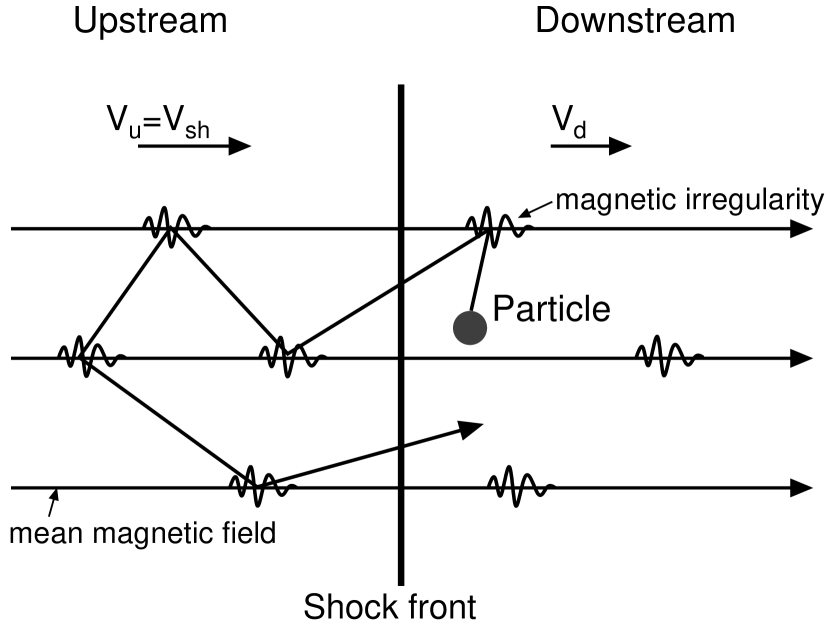
Figure 1: A schematic illustration of the acceleration of a particle in a non-relativistic, parallel shock wave.

From a theoretical viewpoint, the problem of the acceleration process consists of two parts. One is how particles are accelerated for one-cycle of the shock crossings. The other is how the distribution function of the particles evolves when the one-cycle properties are given. The former is determined by details of the scattering process and is quite a difficult problem unless the diffusion approximation is applicable; the properties of both turbulent magnetic field in the vicinity of the shock front and transport of particles in such turbulent fields themselves remain long-standing problems. On the other hand, it is possible to establish a well-defined theory formally for the latter problem. In the present paper, we therefore construct that theory from the point of view of the single particle approach.

2.2 Description as a Markov process

In this paper, we investigate the acceleration process at the shock front; our primary aim is to solve the steady state and time-dependent solution of the distribution function of particles at the shock front. Therefore, we concentrate only on the state of particles, $(\mn@boldsymbol{p},t)$, at the crossing of the shock front, where $\mn@boldsymbol{p}$ is the momentum of a particle and $t$ is the time respectively; we measure $\mn@boldsymbol{p}$ in the downstream frame and $t$ in the shock rest frame, respectively. The history of acceleration process of a particle observed at the shock front can be described by a sequence of the state of the particle at each end of the acceleration cycle, that is, at each shock crossing from the upstream to downstream region:

$$(\mn@boldsymbol{p}_{0},t_{0}),(\mn@boldsymbol{p}_{1},t_{1}),(\mn@boldsymbol{p}_{2},t_{2}),...\ .$$ (2)

Such a sequence is terminated when the particle escapes from the acceleration region, usually from the downstream region. We consider this process in the $\mn@boldsymbol{p}-t$ space where each state of the sequence defines a point, which is called ‘state point’ in the following. If the changes in $\mn@boldsymbol{p}$ and $t$ at each cycle, $(\Delta\mn@boldsymbol{p},\Delta t)$, are stochastic variables as already mentioned, the acceleration process can be regarded as a stochastic process in the $\mn@boldsymbol{p}-t$ space. Usually, this is a Markov process because the changes $(\Delta\mn@boldsymbol{p},\Delta t)$ mostly depend only on the momentum at the last cycle.

Although the history of $(\mn@boldsymbol{p},t)$ provides complete information of the acceleration process at the shock front, we consider only the history of $(p,t)$ in this paper, where $p$ is the magnitude of the momentum, because only $p$ concerns most practical purposes. In order to treat the history of $(p,t)$ solely as a Markov process, we also assume that the probability density of the changes in $p$ and $t$ at one-cycle does not depend on the direction of the momentum at the last cycle, at least approximately. (If this assumption is not appropriate, we must deal with the state of a particle by $(\mn@boldsymbol{p},t)$ or $(p,\mu,t)$, where $\mu$ is the cosine of the angle between the shock normal and the momentum of the particle.) For considering the acceleration of relativistic particles, it is better to describe this process in a logarithmic momentum space, because the changes in $p$ at each cycle are usually multiplicative rather than additive as shown in equation (1). Furthermore, since we consider only mono-energetic injection with a certain momentum of $p_{0}$ measured in the downstream rest frame in the fundamental part of the following description, we use a new quantity

$$q:=\ln(p/p_{0})$$ (3)

instead of $p$ to simplify the description.

Thus, the acceleration process of a particle can be considered as a two-dimensional Markov process on the $q-t$ plane. This stochastic process is described by a probability density function which describes the transition on the $q-t$ plane for one cycle of the acceleration, $\rho(\Delta q,\Delta t;q)$, where $\Delta q$ and $\Delta t$ are respectively the changes in $q$ and $t$ at one-cycle; $q$ in this notation denotes the logarithmic momentum at the last cycle representing the Markov property of this process. (We also use the term ‘step’ instead of ‘cycle’ for the point of view of Markov process in the following.) Since a particle can be lost from the acceleration region at each cycle at a probability of $P_{\mathrm{esc}}(q)$, this density is a defective one; the integration of it over all area is not normalized to unity, but to the return probability, $P_{\mathrm{ret}}(q)=1-P_{\mathrm{esc}}(q)$, as follows:

$$\int_{0}^{\infty}d\Delta q\int_{0}^{\infty}d\Delta t\ \rho(\Delta q,\Delta t;q)=P_{\mathrm{ret}}(q).$$ (4)

In the present paper, for simplicity, we assume $\Delta q>0$, that is, any energy loss mechanisms are not efficient. (However, to generalize the following description to include the possibility of $\Delta q<0$ is not difficult.) The correlation between the energy gain $\Delta q$ and the cycle-time $\Delta t$, which can be considerable for relativistic shocks (see Bednarz & Ostrowski, 1996), can be included in the functional form of $\rho$. For later convenience, we define here the moments of $\Delta q$ and $\Delta t$ as follows:

$$\langle(\Delta q)^{n}\rangle:=\frac{1}{P_{\mathrm{ret}}}\int_{0}^{\infty}d\Delta q\int_{0}^{\infty}d\Delta t\ (\Delta q)^{n}\ \rho(\Delta q,\Delta t;q),$$ (5)

$$\langle(\Delta t)^{n}\rangle:=\frac{1}{P_{\mathrm{ret}}}\int_{0}^{\infty}d\Delta q\int_{0}^{\infty}d\Delta t\ (\Delta t)^{n}\ \rho(\Delta q,\Delta t;q),$$ (6)

$$\sigma_{\Delta q}:=\sqrt{\langle(\Delta q)^{2}\rangle-\langle\Delta q\rangle^{2}},$$ (7)

$$\sigma_{\Delta t}:=\sqrt{\langle(\Delta t)^{2}\rangle-\langle\Delta t\rangle^{2}}.$$ (8)

These quantities are generally dependent on $q$ at the last cycle. As already mentioned, although the functional form of $\rho(\Delta q,\Delta t;q)$ is determined by microscopic physics, we do not specify it and discuss the process formally in this paper (we adopt only an approximate model of $\rho$ in Section 4 and simple toy-models in Section 5).

Defining the probability density function of the state points at $n$th step, $\rho_{n}$, the progress from $(n-1)$th step to $n$th step is expressed by

$$\rho_{n}(q,t)=\int_{0}^{q}dq^{\prime}\int_{0}^{t}dt^{\prime}\ \rho(q-q^{\prime},t-t^{\prime};q^{\prime})\rho_{n-1}(q^{\prime},t^{\prime}).$$ (9)

Again, the integrals of these $\rho_{n}$’s over all area are not normalized to unity, but to the probability at which a particle continues the acceleration cycle at least $n$ times, $P_{n}$:

$$\int_{0}^{\infty}dq\int_{0}^{\infty}dt\ \rho_{n}(q,t)=P_{n}.$$ (10)

Since we consider now the case where particles are all injected at the same state of $(q_{0},t_{0})=(0,0)$, we have

$$\rho_{1}(q,t)=\rho(q,t;q=0).$$ (11)

The integral in equation (9) includes a plain convolution with respect to $t$. It is better to represent such equations in the form of the Laplace transform with respect to $t$. Introducing the following notation

$$\tilde{f}(s):=\int_{0}^{\infty}f(t)\mathrm{e}^{-st}dt,$$ (12)

where $f(t)$ is a function of $t$, equation (9) is transformed to

$$\tilde{\rho}_{n}(q,s)=\int_{0}^{q}\tilde{\rho}(q-q^{\prime},s;q^{\prime})\tilde{\rho}_{n-1}(q^{\prime},s)\ dq^{\prime}.$$ (13)

In a mathematical sense, the above stochastic process can be regarded as a terminating renewal process in the probability theory (cf. Feller, 1971; Cox & Miller, 1965). However, since the present process is two-dimensional and also has a Markov property, it is a more complex problem. Furthermore, the stochastic process defined by equation (13) for a fixed $s$ can be regarded as the random walk process dealt with in the previous paper (Kato & Takahara, 2001), except that the present process is in $q$-space with the Markov property, always increases the value of $q$ and has no absorbing barriers.

2.3 The density of state points

A history of acceleration process of a particle can be represented by plotting the state points on the $q-t$ plane. When such plots are made for many particles and superposed as shown in Fig. 2, we can define the density of the state points:

$$\Psi(q,t):=\sum_{n=1}^{\infty}\rho_{n}(q,t),$$ (14)

where the density is normalized by the number of the particles. This is a key concept to treat the present problem.

Figure 2: A scatter plot of the state points superposed for many particles obtained by Monte Carlo simulations (see Section 4 for details). The unit of time is taken the mean cycle-time for $q=0$. The density of these points defines $\Psi(q,t)$ in equation (14).

The physical meaning of the product $\Psi(q,t)dqdt$ is the expectation value of number of particles which are initially injected at $(q,t)=(0,0)$ and then cross the shock front from the upstream to downstream side within ranges $[q,q+dq]$ and $[t,t+dt]$, per unit injection. We can therefore relate this density with the flux and distribution function of the particles at the shock front (see the following subsection).

Combining equations (9) and (14), we obtain the following integral equation:

$$\Psi(q,t)=\rho(q,t;0)+\int_{0}^{q}dq^{\prime}\int_{0}^{t}dt^{\prime}\rho(q-q^{\prime},t-t^{\prime};q^{\prime})\Psi(q^{\prime},t^{\prime}).$$ (15)

This equation determines $\Psi$ from only $\rho$, and is a fundamental equation to our description. Taking the Laplace transform of this integral equation with respect to $t$, we obtain

$$\tilde{\Psi}(q,s)=\tilde{\rho}(q,s;0)+\int_{0}^{q}\tilde{\rho}(q-q^{\prime},s;q^{\prime})\tilde{\Psi}(q^{\prime},s)\ dq^{\prime}.$$ (16)

For a fixed $s$, this integral equation is regarded as a Volterra equation of the second kind. Since it is generally difficult to solve this equation in analytical form, we will give numerical methods in Section 2.5. In the following, we will use the following relation

$$\int_{0}^{\infty}\Psi(q,t)dt=\tilde{\Psi}_{0}(q),$$ (17)

where $\tilde{\Psi}_{0}(q):=\tilde{\Psi}(q,0)$.

Some quantities related with the acceleration process are described in terms of $\Psi$ as follows. From equations (10) and (14), we obtain

$$\int_{0}^{\infty}dq\int_{0}^{\infty}dt\ \Psi(q,t)=\int_{0}^{\infty}\tilde{\Psi}_{0}(q)\ dq=\sum_{n=1}^{\infty}P_{n}=\langle n\rangle,$$ (18)

where $\langle n\rangle$ is the expectation value of the number of cycles in an acceleration process. (The probability at which a particle continues the cycle just $n$ times before escaping is given by $P_{n}-P_{n+1}$.) The probability at which a particle escapes from the acceleration region before attaining to $q$ for $0<t<\infty$ is given by

$$P_{\mathrm{E}}(q) = P_{\mathrm{esc}}(0)+\int_{0}^{q}dq^{\prime}P_{\mathrm{esc}}(q^{\prime})\int_{0}^{\infty}dt^{\prime}\Psi(q^{\prime},t^{\prime})$$ (19)

$$= P_{\mathrm{esc}}(0)+\int_{0}^{q}P_{\mathrm{esc}}(q^{\prime})\tilde{\Psi}_{0}(q^{\prime})dq^{\prime},$$

because a state point at $q$ does not make the next state point at the probability $P_{\mathrm{esc}}(q)$. We can show $P_{\mathrm{E}}(q)\to 1$ as $q\to\infty$. The probability at which a particle attains to $q$ for $0<t<\infty$ is of course given by $P_{\mathrm{A}}(q)=1-P_{\mathrm{E}}(q)$, and we obtain from equation (19)

$$-\frac{\mathrm{d}P_{\mathrm{A}}(q)}{\mathrm{d}q}=P_{\mathrm{esc}}(q)\tilde{\Psi}_{0}(q).$$ (20)

Note that $P_{\mathrm{A}}(q)$ does not approach unity as $q\to 0$ but to $1-P_{\mathrm{esc}}(0)$ because $\Psi$ includes no contribution from the state points of the particles just injected at $(0,0)$, by its definition. The mean acceleration time for attaining to $q$ is defined by

$$\bar{t}(q):=\frac{\int_{0}^{\infty}t\Psi(q,t)dt}{\int_{0}^{\infty}\Psi(q,t)dt}=-\left.\frac{\partial\tilde{\Psi}}{\partial s}\right|_{s=0}/\tilde{\Psi}_{0}(q).$$ (21)

From the point of view of the renewal process, the density of state points $\Psi$ and the integral equation (15) correspond to the renewal density and the renewal equation, respectively. A concept similar to $\Psi$ was also introduced in the previous paper (Kato & Takahara, 2001) to deal with the random walk of particles.

2.4 Particle distribution function at the shock front

Here, we relate the density of state points introduced in the previous subsection with the particle distribution function at the shock front. We consider the acceleration of relativistic particles in a plane shock, where the velocity of the particles can be approximated by the speed of light $c$ in the shock rest frame and in both fluid frames.

Consider first an impulsive injection of unit particles with $q=0$ at $t=0$ at the shock front. Letting $\mu$ be the cosine of the angle between the shock normal and the direction of particle momentum measured in the shock rest frame, we can define the distribution function of particles at the shock front for this injection, $W_{\mathrm{sf}}(q,\mu,t)$, where $q$ is measured in the downstream rest frame; $\mu$ and $t$ are measured in the shock rest frame. In terms of this function, the one-sided flux of particles with logarithmic momentum $q$ at the shock front from the upstream to the downstream is represented by

$$S_{\mathrm{sf+}}(q,t)=\int_{0}^{1}c\mu\ W_{\mathrm{sf}}(q,\mu,t)d\mu=c\langle\mu\rangle_{+}W_{\mathrm{sf+}}(q,t),$$ (22)

where we introduce the following notations:

$$W_{\mathrm{sf+}}(q,t):=\int_{0}^{1}W_{\mathrm{sf}}(q,\mu,t)d\mu,$$ (23)

$$\langle\mu\rangle_{+}:=\int_{0}^{1}\mu W_{\mathrm{sf}}(q,\mu,t)d\mu\ /\ W_{\mathrm{sf+}}(q,t),$$ (24)

where $\langle\mu\rangle_{+}$ is, in general, dependent on $q$ . On the other hand, as already mentioned, because

$$\Psi(q,t)dt=S_{\mathrm{sf+}}(q,t)dt$$ (25)

for the present situation, we obtain the following relation

$$W_{\mathrm{sf+}}(q,t)=\frac{1}{c\langle\mu\rangle_{+}}\Psi(q,t).$$ (26)

Because this $W_{\mathrm{sf+}}(q,t)$ can be regarded as a Green’s function of the time-dependent solution of the distribution function at the shock front, the solution for more general injection rate $Q(t)$, $F_{\mathrm{sf+}}(q,t)$, is constructed as

$$F_{\mathrm{sf+}}(q,t) = \int_{0}^{t}W_{\mathrm{sf+}}(q,t-t^{\prime})Q(t^{\prime})dt^{\prime}$$ (27)

$$= \frac{1}{c\langle\mu\rangle_{+}}\int_{0}^{t}\Psi(q,t-t^{\prime})Q(t^{\prime})dt^{\prime},$$

where $F_{\mathrm{sf+}}$ is defined from $F_{\mathrm{sf}}$ like $W_{\mathrm{sf+}}$, or in the form of the Laplace transform

$$\tilde{F}_{\mathrm{sf+}}(q,s)=\frac{1}{c\langle\mu\rangle_{+}}\tilde{\Psi}(q,s)\tilde{Q}(s).$$ (28)

In the following, we deal with only the steady injection, that is, $Q(t)=Q_{0}=\mathrm{const}$ for $t\geq 0$ and $Q(t)=0$ for $t<0$. For the case, the steady state solution $(t\to\infty)$ is given by

$$F_{\mathrm{sf+}}(q,\infty)=\frac{Q_{0}}{c\langle\mu\rangle_{+}}\tilde{\Psi}_{0}(q),$$ (29)

using the relation (17). In the following, to simplify the notations, we also express the time-dependent solution in terms of the ‘cut-off function’ defined by

$$\Theta(q,t):=\frac{\int_{0}^{t}\Psi(q,t^{\prime})dt^{\prime}}{\int_{0}^{\infty}\Psi(q,t^{\prime})dt^{\prime}}=\frac{\int_{0}^{t}\Psi(q,t^{\prime})dt^{\prime}}{\tilde{\Psi}_{0}(q)},$$ (30)

resulting in

$$F_{\mathrm{sf+}}(q,t)=F_{\mathrm{sf+}}(q,\infty)\Theta(q,t).$$ (31)

The Laplace transform of this function with respect to $t$ is written by

$$\tilde{\Theta}(q,s)=\frac{1}{s}\frac{\tilde{\Psi}(q,s)}{\tilde{\Psi}_{0}(q)}.$$ (32)

Because $\Psi(q,t)$ always takes non-negative value, we can see that $0\leq\Theta(q,t)\leq 1$ for any values of $(q,t)$ for the steady injection; the time-dependent solution always lies under the envelope of the steady state solution. This function is identical to the function $\phi(t,x,p)$ of Drury (1991) at the shock front $(x=0)$ [see equation (9) of his paper], which was used in the analysis of time-dependent solutions of the diffusion-convection equation.

It should be noted that, in some cases, the steady state solution $F_{\mathrm{sf+}}(q,\infty)$ can be evaluated without introducing the density function $\Psi$. Substituting equation (20) into equation (29), we obtain

$$F_{\mathrm{sf+}}(q,\infty)=\frac{Q_{0}}{c\langle\mu\rangle_{+}P_{\mathrm{esc}}(q)}\left(-\frac{dP_{\mathrm{A}}(q)}{dq}\right).$$ (33)

Therefore, if $P_{\mathrm{A}}(q)$ is estimated by another way, the steady state solution is obtained immediately; conventional single-particle approaches can estimate $P_{\mathrm{A}}(q)$ approximately (e.g. Bell, 1978; Peacock, 1981) and therefore can obtain the steady state solution. Although, to treat the time development of the distribution function, we must treat the function $\Psi$ explicitly.

2.5 Numerical Methods

By numerical methods, the integral equation (16) can be solved straightforwardly (see chapter 18.2 of Press et al. 2002). For a given range $0<q<q_{\mathrm{max}}$, dividing the range into $N$ meshes with uniform intervals of $h:=q_{\mathrm{max}}/N$ and adopting the trapezoidal rule to the integral in the equation, and introducing notations $q_{i}=ih$, $\tilde{\rho}_{ij}:=\tilde{\rho}(q_{i}-q_{j},s;q_{j})$ and $\tilde{\Psi}_{i}:=\tilde{\Psi}(q_{i},s)$ for $i=0,1,...,N$ (we omit the dependence on $s$ for simplicity here), equation (16) is discretized as follows:

$$\tilde{\Psi}_{0}=\tilde{\rho}_{00},$$ (34)

$$\left(1-\frac{h}{2}\tilde{\rho}_{ii}\right)\tilde{\Psi}_{i}=\tilde{\rho}_{i0}+h\left(\frac{1}{2}\tilde{\rho}_{i0}\tilde{\Psi}_{0}+\sum_{j=1}^{i-1}\tilde{\rho}_{ij}\tilde{\Psi}_{j}\right),$$ (35)

where $i=1,2,...,N$. Thus, $\tilde{\Psi}_{i}$’s are trivially solved by forward substitution. Note that the interval $h$ must be fine enough to resolve the kernel $\tilde{\rho}$.

Once $\tilde{\Psi}(q,s)$ is obtained by this way for each $s$, we can then make a numerical inversion of Laplace transform described in Appendix A to obtain $\Psi(q,t)$. We can also obtain $F_{\mathrm{sf+}}(q,t)$ for general injection or $\Theta(q,t)$ for steady injection numerically by inverting equation (28) or (32), respectively.

3 Self-similar solution of particle distribution

One of the most well-known features of the first-order Fermi acceleration is the power-law distribution function of accelerated particles in steady state. Theoretically, it is just a consequent of some scaling laws, or similarities, in the one-cycle probability density function $\rho$; in theoretical studies on the first-order Fermi acceleration, such a scaling law is usually assumed implicitly or explicitly. The scaling-law may realize when, for example, the power spectrum of the turbulent magnetic field has a power-law feature. The fact that the power-law distribution is really observed in various shocks may indicate such a scaling law often realizes well. In the following, we also examine such a case in an analytical way.

3.1 One-step probability density function with a scaling law

We consider here the case in which the transition of each step $(\Delta q,\Delta t)$ satisfies the following scaling law; for normalized variables $\Delta q$ and $\Delta t/(p/p_{0})^{\alpha}(=\mathrm{e}^{-\alpha q}\Delta t)$, where $\alpha$ is a constant parameter, the probability distribution function defined for these variables is independent of $q$ at the last step or, in other words, common for all $q$. This means that the one-step probability density $\rho(\Delta q,\Delta t;q)$ can be represented by a single function $\varphi(\Delta q,\mathrm{e}^{-\alpha q}\Delta t)$ as

$$\rho(\Delta q,\Delta t;q)=\mathrm{e}^{-\alpha q}\varphi(\Delta q,\mathrm{e}^{-\alpha q}\Delta t)$$ (36)

and

$$\tilde{\rho}(\Delta q,s;q)=\tilde{\varphi}\left(\Delta q,e^{\alpha q}s\right).$$ (37)

The similarity of this function is clear. Note that $P_{\mathrm{ret}}(q)$, $P_{\mathrm{esc}}(q)$ and the moments of $\Delta q$ are all independent of $q$:

$$P_{\mathrm{ret}}=\int_{0}^{\infty}\tilde{\varphi}_{0}(\Delta q)d\Delta q=\mathrm{const}$$ (38)

and

$$\langle(\Delta q)^{n}\rangle=\frac{1}{P_{\mathrm{ret}}}\int_{0}^{\infty}(\Delta q)^{n}\tilde{\varphi}_{0}(\Delta q)d\Delta q=\mathrm{const},$$ (39)

where $\tilde{\varphi}_{0}(\Delta q):=\tilde{\varphi}(\Delta q,s=0)$. The integral equation (16) is reduced to

$$\tilde{\Psi}(q,s)=\tilde{\varphi}(q,s)+\int_{0}^{q}\tilde{\varphi}(q-q^{\prime},\mathrm{e}^{\alpha q^{\prime}}s)\tilde{\Psi}(q^{\prime},s)\ dq^{\prime}.$$ (40)

3.2 Steady state solution

3.2.1 Power-law solution

We first consider the steady state solution here. Setting $s=0$ in equation (40), we have

$$\tilde{\Psi}_{0}(q)=\tilde{\varphi}_{0}(q)+\int_{0}^{q}\tilde{\varphi}_{0}(q-q^{\prime})\tilde{\Psi}_{0}(q^{\prime})\ dq^{\prime}.$$ (41)

Again, denoting the Laplace transform with respect to $q$ by

$$f^{*}(\theta):=\int_{0}^{\infty}f(q)e^{-\theta q}dq,$$ (42)

where $f(q)$ is a function of $q$, we can write the exact solution of equation (41) in the form of the Laplace transform as follows

$$\tilde{\Psi}^{*}_{0}(\theta)=\frac{\tilde{\varphi}^{*}_{0}(\theta)}{1-\tilde{\varphi}^{*}_{0}(\theta)}.$$ (43)

As well known, the inversion of this transform is given through the Bromwich integral on the complex $\theta$-plane:

$$\tilde{\Psi}_{0}(q)=\frac{1}{2\pi\mathrm{i}}\int_{\gamma-\mathrm{i}\infty}^{\gamma+\mathrm{i}\infty}\frac{\tilde{\varphi}^{*}_{0}(\theta)}{1-\tilde{\varphi}^{*}_{0}(\theta)}\mathrm{e}^{\theta q}d\theta,$$ (44)

where $\gamma$ is a real constant taken so that the vertical line $\mathrm{Re}(\theta)=\gamma$ lies on the right of the all poles of $\tilde{\varphi}^{*}_{0}(\theta)/[1-\tilde{\varphi}^{*}_{0}(\theta)]$. While the numerical solution can be obtained directly (see Appendix A), we investigate the asymptotic behaviour of equation (44) here.

Assuming that $\tilde{\varphi}^{*}_{0}(\theta)\to 0$ as $|\theta|\to\infty$ (we expect this condition usually holds), the contour of the integral in the last equation is closed through the left of the $\theta$-plane. The integrand obviously has poles at the points where the condition $\tilde{\varphi}^{*}_{0}(\theta)=1$ is satisfied. Because $\tilde{\varphi}^{*}_{0}(0)=P_{\mathrm{ret}}<1$ and

$$\frac{\mathrm{d}\tilde{\varphi}^{*}_{0}}{\mathrm{d}\theta}=-\int_{0}^{\infty}\Delta q\tilde{\varphi}_{0}(\Delta q)e^{-\theta\Delta q}d\Delta q<0,$$ (45)

the equation $\tilde{\varphi}^{*}_{0}(\theta)=1$ has the unique negative root on the real axis of the complex $\theta$-plane. We write this root as $\theta_{-}$. As $q$ becomes sufficiently large, because only the pole at $\theta_{-}$ dominantly contributes to the integral (44), we obtain the asymptotic solution $(q\to\infty)$

$$\tilde{\Psi}_{0}(q)\sim A^{-1}\mathrm{e}^{-\lambda q},$$ (46)

where $\lambda:=-\theta_{-}$ ($\lambda>0$) and

$$A:=-\left.\frac{\mathrm{d}\tilde{\varphi}^{*}_{0}}{\mathrm{d}\theta}\right|_{\theta=-\lambda}=\int_{0}^{\infty}\Delta q\tilde{\varphi}_{0}(\Delta q)\mathrm{e}^{\lambda\Delta q}d\Delta q.$$ (47)

The index $\lambda$ is, by definition of $\theta_{-}$, determined as the unique positive root of

$$\int_{0}^{\infty}\tilde{\varphi}_{0}(\Delta q)\mathrm{e}^{\lambda\Delta q}d\Delta q=1.$$ (48)

Recalling $q=\ln(p/p_{0})$, the steady state solution (29) for large $q$ is written by

$$F^{(p)}_{\mathrm{sf+}}(p,\infty)\sim\frac{Q_{0}}{Ac\langle\mu\rangle_{+}}\frac{1}{p_{0}}\left(\frac{p}{p_{0}}\right)^{-(1+\lambda)},$$ (49)

where $F^{(p)}_{\mathrm{sf+}}(p)dp=F_{\mathrm{sf+}}(q=\ln(p/p_{0}))dq$. This is the power-law solution whose index is given by $\sigma=1+\lambda$.

3.2.2 Approximations

If the dispersion of $\Delta q$, $\sigma_{\Delta q}$, is negligible in equations (48) and (47), namely $\sigma_{\Delta q}\ll\lambda^{-1}$, we can approximate $\tilde{\varphi}_{0}(q)=P_{\mathrm{ret}}\delta(q-\langle\Delta q\rangle)$ there, resulting in

$$\lambda=-\frac{\ln P_{\mathrm{ret}}}{\langle\Delta q\rangle}.$$ (50)

This expression is equivalent to equation (5) of Peacock (1981). We will mention the validity of this formula again in Section 5. The condition to use this approximation can be rewritten as

$$\frac{\langle\Delta q\rangle}{\sigma_{\Delta q}}\gg-\ln P_{\mathrm{ret}}.$$ (51)

Furthermore, if $\sigma_{\Delta q}\ll\langle\Delta q\rangle$, we have

$$A=\langle\Delta q\rangle.$$ (52)

On the other hand, if $\langle\Delta q\rangle\ll\lambda^{-1}$ and $\sigma_{\Delta q}\ll\lambda^{-1}$, expanding $\exp(\lambda q)$ to the first-order of $\lambda q$ in both equations (48) and (47), we obtain

$$\lambda=\frac{P_{\mathrm{esc}}}{P_{\mathrm{ret}}\langle\Delta q\rangle},\qquad A=P_{\mathrm{ret}}\langle\Delta q\rangle.$$ (53)

As shown in Section 4, this approximation is applicable to the acceleration in non-relativistic shocks.

3.3 Time-dependent solution

3.3.1 Self-similarity

Here, we show that the time-dependent solution of equation (40) has a self-similarity for $q\gg\langle\Delta q\rangle$. Firstly, for $q\gg\langle\Delta q\rangle$, we have approximately

$$\tilde{\Psi}(q,s)=\int_{0}^{q}\tilde{\varphi}(q-q^{\prime},e^{\alpha q^{\prime}}s)\tilde{\Psi}(q^{\prime},s)dq^{\prime}.$$ (54)

This equation must be regarded as a relation for large $q$, not as an integral equation defined over all region of $q$; such an integral equation would have only a trivial zero solution. For a positive constant $a$, it is seen that the function defined by

$$\tilde{\Psi}_{a}(q,s):=\tilde{\Psi}(q+\ln a,a^{-\alpha}s)$$ (55)

also satisfies the above relation instead of $\tilde{\Psi}$; in other word, the relation does not change its form under the transformation $q\to q+\ln a$ and $s\to a^{-\alpha}s$ simultaneously. Secondly, the steady state solution (46), which is regarded as a ‘boundary condition’ at $s=0$, is only multiplied by the constant $a^{-\lambda}$ under this transformation. Finally, because the relation (54) is linear, we obtain the following self-similarity of the density of state points for $q\gg\langle\Delta q\rangle$:

$$\tilde{\Psi}(q+\ln a,a^{-\alpha}s)=a^{-\lambda}\tilde{\Psi}(q,s),$$ (56)

$$\Psi(q+\ln a,a^{\alpha}t)=a^{-(\alpha+\lambda)}\Psi(q,t).$$ (57)

For the cut-off function, we obtain

$$\Theta(q+\ln a,a^{\alpha}t)=\Theta(q,t).$$ (58)

Defining functions for $p$ instead of $q$, $\Psi^{(p)}(p)dp:=\Psi(q=\ln(p/p_{0}))dq$ and $\Theta^{(p)}(p):=\Theta(q=\ln(p/p_{0}))$, we obtain

$$\Psi^{(p)}(ap,a^{\alpha}t)=a^{-(1+\alpha+\lambda)}\Psi^{(p)}(p,t),$$ (59)

$$\Theta^{(p)}(ap,a^{\alpha}t)=\Theta^{(p)}(p,t).$$ (60)

For later convenience, we derive a relation between the steady state solution and the time-dependent solution here. Because $\varphi(q,t)$ is usually a concentrated function of $t$, the Laplace transform of it, $\tilde{\varphi}(q,s)$, has a characteristic value of $s=s_{*}$ so that $\tilde{\varphi}(q,s)$ can be approximated by $\tilde{\varphi}_{0}(q)$ for $s<s_{*}$. Therefore, in the region of $q-s$ plane where the condition $\mathrm{e}^{\alpha q}s<s_{*}$ is satisfied, the integral equation (40) is approximated by

$$\tilde{\Psi}(q,s)=\tilde{\varphi}_{0}(q)+\int_{0}^{q}\tilde{\varphi}_{0}(q-q^{\prime})\tilde{\Psi}(q^{\prime},s)dq^{\prime},$$ (61)

resulting in $\tilde{\Psi}(q,s)\sim\tilde{\Psi}_{0}(q)$ in that region. Thus, we can define

$$q_{*}(s):=\frac{1}{\alpha}\ln(s_{*}/s)$$ (62)

so that we have $\tilde{\Psi}(q,s)\sim\tilde{\Psi}_{0}(q)$ for $s<s_{*}$ and $q<q_{*}(s)$.

3.3.2 Approximate solution

When $\tilde{\Psi}$ varies with $q$ much more slowly than $\tilde{\varphi}$, we can approximate in the integrand of equation (40) as

$$\tilde{\Psi}(q^{\prime},s)\sim\tilde{\Psi}(q,s)+(q^{\prime}-q)\frac{\partial\tilde{\Psi}}{\partial q}(q,s).$$ (63)

A rough criterion to use this approximation may be given by $\langle\Delta q\rangle\ll\lambda^{-1}$ and $\sigma_{\Delta q}\ll\lambda^{-1}$, since the typical variation scale of $\Psi$ is given by $\lambda^{-1}$ for the steady state solution (46). Thus, for $q\gg\langle\Delta q\rangle$, the integral equation (40) is reduced to

$$\tilde{\Psi}(q,s)=B_{1}(q,s)\tilde{\Psi}(q,s)-B_{2}(q,s)\frac{\partial\tilde{\Psi}}{\partial q}(q,s),$$ (64)

where

$$B_{1}(q,s) := \int_{0}^{\infty}\tilde{\varphi}(\Delta q,\mathrm{e}^{\alpha q}s)d\Delta q,$$ (65)

$$B_{2}(q,s) := \int_{0}^{\infty}\Delta q\tilde{\varphi}(\Delta q,\mathrm{e}^{\alpha q}s)d\Delta q.$$ (66)

For a fixed $s$, equation (64) can be regarded as an ordinary differential equation for $\tilde{\Psi}$, and the solution is given by

$$\tilde{\Psi}(q,s)=C(s)\exp\left[-\int_{q_{0}(s)}^{q}\frac{1-B_{1}(q^{\prime},s)}{B_{2}(q^{\prime},s)}dq^{\prime}\right],$$ (67)

where $C(s)$ and $q_{0}(s)$ are functions of $s$; we can choose the function $q_{0}(s)$ arbitrarily here. If we choose $q_{0}(s)=q_{*}(s)$, which was defined in equation (62), we can determine $C(s)=\tilde{\Psi}_{0}(q_{*}(s))$, because $\tilde{\Psi}(q,s)=\tilde{\Psi}_{0}(q)$ for $q\leq q_{*}(s)$. Thus, the solution is written by

$$\tilde{\Psi}(q,s)=\tilde{\Psi}_{0}(q_{*}(s))\exp\left[-\int_{q_{*}(s)}^{q}\frac{1-B_{1}(q^{\prime},s)}{B_{2}(q^{\prime},s)}dq^{\prime}\right].$$ (68)

It is easily seen that the above expression satisfies the similarity (56), because $B_{1}(q+\ln a,a^{-\alpha}s)=B_{1}(q,s)$, $B_{2}(q+\ln a,a^{-\alpha}s)=B_{2}(q,s)$ and $q_{*}(a^{-\alpha}s)=q_{*}(s)+\ln a$. For $q<q_{*}(s)$, because $B_{1}(q,s)=P_{\mathrm{ret}}$ and $B_{2}(q,s)=P_{\mathrm{ret}}\langle\Delta q\rangle$, we obtain

$$\int_{q_{*}(s)}^{q}\frac{1-B_{1}(q^{\prime},s)}{B_{2}(q^{\prime},s)}dq^{\prime}=\frac{P_{\mathrm{esc}}}{P_{\mathrm{ret}}\langle\Delta q\rangle}(q-q_{*}(s)),$$ (69)

which is consistent with the steady state solution (46) with $\lambda$ of equation (53). For $q\gg\langle\Delta q\rangle$, where the asymptotic solution (46) is applicable for steady state, we finally obtain the following asymptotic expression

$$\tilde{\Psi}(q,s)=A^{-1}\mathrm{e}^{-I(q,s)},$$ (70)

where

$$I(q,s):=\int_{0}^{q}\frac{1-B_{1}(q^{\prime},s)}{B_{2}(q^{\prime},s)}dq^{\prime}.$$ (71)

We will use this approximation in the following section. Although it is usually difficult to invert the above expressions analytically, it is able to do it numerically (see Appendix A). Under the above approximation, the mean acceleration time defined by (21) is represented by

$$\bar{t}(q)=\frac{\mathrm{e}^{\alpha q}-1}{\alpha P_{\mathrm{ret}}\langle\Delta q\rangle}\langle\Delta t\rangle_{0},$$ (72)

where $\langle\Delta t\rangle_{0}$ denotes the mean cycle-time $\langle\Delta t\rangle$ for $q=0$.

4 Application to non-relativistic shocks

In order to confirm that our method surely reproduces the well-known results, we apply the method to the acceleration in non-relativistic shocks in this section. We consider a simple one-dimensional parallel shock as in Fig. 1 with shock speed $V_{\mathrm{sh}}$($\ll c$). The fluid speeds in the upstream and downstream region measured in the shock rest frame are denoted by $V_{\mathrm{u}}$ and $V_{\mathrm{d}}$, respectively, and are assumed uniform in each region. The compression ratio is given by $r=V_{\mathrm{u}}/V_{\mathrm{d}}$.

4.1 One-step probability density function

When we apply our method to a specific case, we must first specify the one-step probability density $\rho$. Assuming that $\rho$ obeys the scaling law (36) discussed in the previous section, we derive here an approximate expression of $\varphi$ applicable to non-relativistic shocks, by a practical way.

First, because the changes in $q$ and $t$ at one-cycle are expected to be mutually independent, the dependences of $\varphi$ on $\Delta q$ and $\Delta t$ can be separable as $\varphi(\Delta q,\Delta t)=\varphi_{q}(\Delta q)\varphi_{t}(\Delta t)$. Since the particle distribution function at the shock front is approximately isotropic, we have

$$\langle\Delta q\rangle\sim\frac{4}{3}\frac{V_{\mathrm{u}}-V_{\mathrm{d}}}{c},\quad\sigma_{\Delta q}\sim\frac{1}{3}\frac{V_{\mathrm{u}}-V_{\mathrm{d}}}{c}.$$ (73)

[cf. equation (1), or equation (7) of Bell 1978]. These two quantities are expected to be small enough, compared with $\lambda^{-1}$, to use the approximations described in Sections 3.2.2 and 3.3.2. Therefore, using these approximations, we can proceed without specifying the functional form of $\varphi_{q}$ here.

The time dependent part $\varphi_{t}$ can be approximated as follows with the aid of a solution of the diffusion-convection equation and results of Monte Carlo simulations. In a one-dimensional diffusion process with a diffusion coefficient $D$ in a moving medium with speed $V$, the time distribution function for returning from a distant point at $x=a$ ($a>0$) to a barrier located at $x=0$ is given by

$$g(t)=\frac{a}{\sqrt{4\pi Dt^{3}}}\exp\left[-\frac{(a+Vt)^{2}}{4Dt}\right]$$ (74)

or in the form of the Laplace transform

$$\tilde{g}(s)=\exp\left\{-\frac{a}{2D}\left[V+(V^{2}+4Ds)^{1/2}\right]\right\}$$ (75)

(see Cox & Miller, 1965; Lagage & Cesarsky, 1983), where $V$ can be positive or negative and, for the present problem, $V=-V_{\mathrm{u}}$ for the upstream region and $V=V_{\mathrm{d}}$ for the downstream region. Since this function already includes the influence of the escape of particles, the return probability is given by

$$P_{\mathrm{ret}}(a)=\tilde{g}(0)=\left\{\begin{array}[]{ll}1&\mbox{for $V<0$}\\ \exp(-aV/D)&\mbox{for $V>0$.}\end{array}\right.$$ (76)

First two moments of the return time $t$ are given by

$$\langle t\rangle=\frac{a}{|V|},\qquad\langle t^{2}\rangle-\langle t\rangle^{2}=\frac{2aD}{|V|^{3}}.$$ (77)

However, the above results are not applicable directly to calculate the cycle-time; in order to do this, we need the distribution of the residence time, that is, the time between entering one of the fluid regions and leaving the region through the shock front, in each region. Here, we employ Monte Carlo simulations to obtain an approximate expression for the residence time distribution. It is known that, in non-relativistic shocks, the properties of particle motion have little dependence on the details of the scattering process. Thus, we can utilize the large-angle scattering model, which was dealt with the previous paper (Kato & Takahara, 2001), in the simulation to estimate the residence time for isotropic injection of particles at the shock front. Performing the Monte Carlo simulations, we found that the distribution of the residence time for isotropic injection at the boundary is approximated well by $g(t)$ in equation (74) if we set the parameters for the diffusion process as follows:

$$a=\frac{4}{3}c\tau_{0},\qquad D=\frac{1}{3}c^{2}\tau_{0},$$ (78)

where $\tau_{0}$ is the mean free time of the particles, defined for the large-angle scattering model, measured in the fluid rest frame. Thus, we can use $g(t)$ with $a=4D/c$ as an approximation of the residence time distribution for each region. Taking the convolution between the residence time distributions for the upstream and downstream region, we finally obtain the distribution of the cycle-time in the form of Laplace transform

$$\tilde{\varphi}_{t}(s)\sim\tilde{G}(s)=\exp\Bigl{\{}-2\bigl{[}\nu_{\mathrm{d}}-\nu_{\mathrm{u}}+(\nu_{\mathrm{u}}^{2}+\frac{4D_{\mathrm{u}}}{c^{2}}s)^{1/2}$$

$$+(\nu_{\mathrm{d}}^{2}+\frac{4D_{\mathrm{d}}}{c^{2}}s)^{1/2}\bigr{]}\Bigr{\}},$$ (79)

where $\nu_{\mathrm{u}}:=V_{\mathrm{u}}/c$ and $\nu_{\mathrm{d}}:=V_{\mathrm{d}}/c$; the diffusion coefficients in the upstream and downstream region are denoted by $D_{\mathrm{u}}$ and $D_{\mathrm{d}}$, respectively. Fig. 3 shows the cycle-time distribution calculated for $V_{\mathrm{u}}=0.01c$ and $r=4$, where we take $D_{\mathrm{u}}=D_{\mathrm{d}}=D$. The solid curve represents the result obtained by inverting equation (79) numerically and the dots are the results from the Monte Carlo simulation. We see that the approximation fits the simulation results quite well. Note that, this distribution is very skew and peaks at $t\ll\langle\Delta t\rangle$, which are prominent features of the diffusion process owing to the random walk motion of the particles.

Figure 3: Time distribution for one-cycle of particles in a non-relativistic shock with $V_{\mathrm{sh}}=0.01c$, $r=4$. The solid curve is the approximate solution, $G(t)$, obtained by inverting equation (79) numerically. The dots are results from a Monte Carlo simulation.

Thus, we can write an approximated form of $\tilde{\varphi}$:

$$\tilde{\varphi}(\Delta q,s)=\varphi_{q}(\Delta q)\tilde{G}(s)$$ (80)

with the quantities in (73). Obviously, the return probability at one-cycle is given by

$$P_{\mathrm{ret}}=\tilde{G}(0)=\exp(-4\nu_{\mathrm{d}})\sim 1-4\nu_{\mathrm{d}},$$ (81)

which is essentially in agreement with the previous results (e.g. Bell, 1978). The first two moments of the cycle-time are given by

$$\langle\Delta t\rangle=\frac{4}{c}\left(\frac{D_{\mathrm{u}}}{V_{\mathrm{u}}}+\frac{D_{\mathrm{d}}}{V_{\mathrm{d}}}\right),\qquad\sigma_{\Delta t}^{2}=\frac{8}{c}\left(\frac{D_{\mathrm{u}}^{2}}{V_{\mathrm{u}}^{3}}+\frac{D_{\mathrm{d}}^{2}}{V_{\mathrm{d}}^{3}}\right).\\$$ (82)

The former result coincides with the previous result derived from the diffusion-convection equation (Drury, 1983). The state points shown in Fig. 2 were also obtained by the Monte Carlo simulations performed above with the same parameter as in Fig. 3.

4.2 Steady state and time-dependent solution

Because of the isotropy of the particle distribution at the shock front, we have

$$F_{\mathrm{sf+}}(q,t)=\frac{1}{2}F_{\mathrm{sf}}(q,t),\qquad\langle\mu\rangle_{+}=\frac{1}{2}.$$ (83)

Because $\langle\Delta q\rangle\ll 1$ and $P_{\mathrm{ret}}\sim 1$, using the approximations in (53), we obtain

$$\lambda\sim\frac{P_{\mathrm{esc}}}{\langle\Delta q\rangle}\sim\frac{3}{r-1},\qquad A\sim\langle\Delta q\rangle\sim\frac{4}{3}\frac{V_{\mathrm{u}}-V_{\mathrm{d}}}{c}.$$ (84)

Substituting the above results into equation (49), the steady state solution for large $p$ is given by

$$F_{\mathrm{sf}}^{(p)}(p,\infty)=\frac{3Q_{0}}{V_{\mathrm{u}}-V_{\mathrm{d}}}\frac{1}{p_{0}}\left(\frac{p}{p_{0}}\right)^{-\sigma}$$ (85)

with $\sigma=(r+2)/(r-1)$, where $F_{\mathrm{sf}}^{(p)}(p)dp=F_{\mathrm{sf}}(q=\ln(p/p_{0}))dq$. In terms of the isotropic part of the usual phase-space distribution function $f(p,x,t)$, where $x$ is distance from the shock front, we have the following relation:

$$f(p,0,t)=\frac{1}{4\pi p^{2}}F_{\mathrm{sf}}(p,t)=\frac{1}{4\pi p^{3}}F_{\mathrm{sf}}(q,t).$$ (86)

We therefore obtain

$$f(p,0,\infty)=\frac{3Q_{0}^{\prime}}{V_{\mathrm{u}}-V_{\mathrm{d}}}\frac{1}{p_{0}}\left(\frac{p}{p_{0}}\right)^{-(\sigma+2)},$$ (87)

where $Q_{0}^{\prime}$ is the mono-energetic, isotropic injection rate defined for $f(p,0,t)$, with which $(df/dt)_{\mathrm{inj}}=Q_{0}^{\prime}\delta(p-p_{0})$ at the shock front. Note that, $Q_{0}^{\prime}$ has the following relation with $Q_{0}$:

$$Q_{0}^{\prime}=\frac{1}{4\pi p_{0}^{2}}Q_{0}.$$ (88)

The above result (87) is equivalent to the previous results [e.g. equation (3.24) of Drury 1983 ].

The time-dependent solution is obtained as follows. Adopting the approximation (70), we can obtain the solution of $\tilde{\Psi}(q,s)$ with

$$B_{1}(q,s)\sim\tilde{G}(\mathrm{e}^{\alpha q}s),\qquad B_{2}(q,s)\sim\langle\Delta q\rangle\tilde{G}(\mathrm{e}^{\alpha q}s),$$ (89)

$$I(q,s)=\frac{-q}{\langle\Delta q\rangle}+\frac{1}{\langle\Delta q\rangle}\int_{0}^{q}\frac{1}{\tilde{G}(\mathrm{e}^{\alpha q^{\prime}}s)}dq^{\prime}.$$ (90)

Then, $\tilde{\Theta}(q,s)$ is given by equation (32). Inverting these results numerically, we finally obtain $\Psi(q,t)$ and $\Theta(q,t)$. Fig. 4 represents the time development of $\Psi(q,t)$ calculated for $V_{\mathrm{sh}}=0.01c$, $r=4$, $\alpha=1$, $D_{\mathrm{u}}=D_{\mathrm{d}}=D$ and $t=500,5000,50000$ in the unit of $\langle\Delta t\rangle_{0}$. The self-similarity given by equation (57) is evident. Fig. 5 represents the time development of $\Theta(q,t)$ calculated for the same parameters as in Fig. 4 except that $t=100,500,2500$. The solutions given by the present method (solid curves) fit the results from Monte Carlo simulations (dots) quite well.

It is interesting to make a comparison between the cut-off function by our method and that by the approximation of Drury (1991). The first two cumulants $c_{1},c_{2}$ in his approximation [see equations (25) and (26) in his paper] are determined as follows. In the present situation, the diffusion coefficients are expressed as $D_{\mathrm{u}}=D_{\mathrm{d}}=D_{0}p/p_{0}$, where $D_{0}$ is the diffusion coefficient for particles with the injection momentum $p_{0}$. From equation (82) we can determine $D_{0}$ in terms of $\langle\Delta t\rangle_{0}$ as

$$D_{0}=\frac{c}{4}\left(\frac{1}{V_{\mathrm{u}}}+\frac{1}{V_{\mathrm{d}}}\right)^{-1}\langle\Delta t\rangle_{0}.$$ (91)

Using this relation, we determine for the present situation

$$c_{1}=\frac{3c}{4V_{\mathrm{sh}}}\frac{r}{r-1}\left(p/p_{0}-1\right)\langle\Delta t\rangle_{0},$$ (92)

$$c_{2}=\frac{3c^{2}}{16V_{\mathrm{sh}}^{2}}\frac{r(r^{3}+1)}{(r-1)(r+1)^{2}}\left[(p/p_{0})^{2}-1\right]\langle\Delta t\rangle_{0}^{2}.$$ (93)

Substituting these results into equation (22) of Drury (1991), we obtain the approximated cut-off function represented in Fig. 5 by dotted curves. As mentioned in his paper, this approximation do not provide satisfactory fits for high energy tail of the distributions, while it provides fairly good fits for lower energies [see also fig. 4 of his paper].

Figure 4: Time development of the density of state points $\Psi(q,t)$ for a non-relativistic shock with $V_{\mathrm{sh}}=0.01c$ and $r=4$. We take $\alpha=1$, $D_{\mathrm{u}}=D_{\mathrm{d}}$ and $t=500,5000,50000$, where the unit of time is the mean cycle-time for $q=0$. The self-similarity given by equation (57) is evident for large $q$.

Figure 5: Time development of the cut-off function $\Theta(q,t)$. The parameters are the same as in Fig. 4, except that t=100, 500, 2500. The solid curves are numerically inverted solutions by the present method, and the dots are results from Monte Carlo simulations. The dotted curves are the approximate solution of Drury (1991).

5 Relation between the one-cycle properties and particle distribution

Recently, the acceleration of particles in ultrarelativistic shocks has attracted some attention in relation to the ultrahigh-energy cosmic rays or high-energy particles at the external shocks associated with gamma-ray bursts. Many works on this issue (theories and simulations) showed that in such shocks the energy gain at one-cycle is approximately given by $\Delta q\sim\ln 2$, owing to the characteristics of the trajectory of particles in the upstream region, and the power-law index is typically given by $\sigma\sim 2.2$ (e.g. Bednarz & Ostrowski, 1998; Kirk et al., 2000; Achterberg et al., 2001). The deviation of $\Delta q$, $\sigma_{\Delta q}$, becomes the same order of $\langle\Delta q\rangle$. Although Peacock’s formula (50) has been often used in the literature to calculate the power-law index (e.g. Kato & Takahara, 2001; Achterberg et al., 2001), it can deviate from the true value because the criterion (51) may not hold in this situation. In addition, it has been shown that the cycle-time can be dominated by the upstream residence time (Gallant & Achterberg, 1999; Achterberg et al., 2001). Because the distribution of the upstream residence time in ultrarelativistic shocks can be much different from that of non-relativistic shocks (cf. Fig. 3 and fig.10 of Achterberg et al. 2001), the feature of the cut-off function can be also different from that of non-relativistic shocks considerably.

To give some insights into these issues, we briefly investigate here how the properties of the one-step probability density function, that is, the stochastic properties of $\Delta q$ and $\Delta t$, affect the shape of the resulting particle distribution, for several toy models. We assume the scaling law (36) discussed in Section 3 and the following separable form

$$\varphi(\Delta q,\Delta t)=\varphi_{q}(\Delta q)\varphi_{t}(\Delta t).$$ (94)

For the following all models, we adopt $P_{\mathrm{ret}}=0.5$, $\langle\Delta q\rangle=\ln 2$, $\langle\Delta t\rangle_{0}=1$ and $\alpha=1$. First, in order to investigate the influence of the dispersion of $\Delta q$, we consider the following two simple models:

$$\varphi_{q}(\Delta q)=\displaystyle\frac{H(\Delta q)-H(\Delta q-2\langle\Delta q\rangle)}{2\langle\Delta q\rangle}$$ (95)

(model 1), and

$$\varphi_{q}(\Delta q)=\displaystyle\frac{H(\Delta q-\langle\Delta q\rangle/2)-H(\Delta q-3\langle\Delta q\rangle/2)}{\langle\Delta q\rangle}$$ (96)

(model 2), where $H(x)$ is the unit step function: $H(x)=0$ for $x<0$, $H(x)=1$ for $x>0$ and $H(x)=1/2$ for $x=0$. The standard deviation of $\Delta q$ for model 2 is a half of that for model 1. For both models, we adopt

$$\varphi_{t}(\Delta t)=P_{\mathrm{ret}}\displaystyle\frac{H(\Delta t)-H(\Delta t-2\langle\Delta t\rangle)}{2\langle\Delta t\rangle}.$$ (97)

These models may represent typical features of the energy-gain and cycle-time in ultrarelativistic shocks which were examined by Achterberg et al. (2001) by Monte Carlo simulations. For model 1, solving equation (48) numerically, we obtain the power-law index of $\lambda\sim 0.91$, while model 2 gives $\lambda\sim 0.98$. This result explicitly shows that the power-law index $\lambda$ is generally dependent not only on $\langle\Delta q\rangle$ but also on the dispersion $\sigma_{\Delta q}$, although this fact is rather evident from equation (48). Because the criterion (51) is not satisfied for both models, especially for model 1, Peacock’s formula (50), which gives $\lambda=1$ for both models, deviates from the true value. [the dispersion of $\Delta q$ is neglected in the derivation of equation (50) and that of Peacock (1981).] This fact may also be responsible for the small discrepancy in the power-law indices in fig.14 of the previous paper (Kato & Takahara, 2001) between our results, which utilized the formula (50), and those of Ellison, Jones & Reynolds (1990), which were determined by fitting results from Monte Carlo simulations. Fig. 6 (a) shows the steady state and time-dependent solutions of the distribution function of particles (in an arbitrary unit) and Fig. 6 (b) shows the cut-off functions, for both models. These solutions are obtained by the numerical method given in Section 2.5. The time-dependent solutions are calculated at $t=10^{3}$. It is seen that model 2 (dotted curve) has a sharper cut-off than model 1 (solid curve), owing to the smaller dispersion of $\Delta q$ than that of model 1.

Figure 6: The distribution function of particles at the shock front for steady injection (a), and the cut-off function (b). The time-dependent solutions are calculated at $t=10^{3}$. The solid curves denote model 1 and the dotted curves denote model 2.

Then, we investigate the influence of the dispersion of $\Delta t$ on the distribution function. We define model 3, which has a ‘diffusive’ nature on the cycle-time, by

$$\varphi_{t}(\Delta t)=P_{\mathrm{ret}}g(\Delta t)/\exp(-4V/c),$$ (98)

where $g(t)$ was defined in equation (74). Although $g(t)$ was derived from the diffusion-convection equation for the return-time distribution function, not for the cycle-time, it may partly represent essential behaviour of the cycle-time distribution for the present situation when the motion of particles is mainly diffusive. In this equation, we use the normalized distribution $g(\Delta t)/\exp(-4V/c)$, where $V=0.01c$, $a=V\langle\Delta t\rangle_{0}$ and $D=cV\langle\Delta t\rangle_{0}/4$ so that $\langle\Delta t\rangle_{0}=1$ [cf. equations (76)–(78)], and take the return probability $P_{\mathrm{ret}}=0.5$ independently. $\varphi_{q}(\Delta q)$ is taken the same as in model 1; the spectral index $\lambda$ of model 3 therefore equals to that of model 1. Fig. 7 (a) shows the distribution function of particles and (b) the cut-off function, for model 1 (solid curve) and model 3 (dotted curve) as in Fig. 6. Although both models have the same mean cycle-time $\langle\Delta t\rangle$, the shapes of high-energy tails are considerably different. This is attributed to the large dispersion of $\Delta t$ in model 3.

Figure 7: The same as Fig. 6 except that the dotted curves denote model 3. Although both models have the same mean cycle-time, the shape of the high energy tails are considerably different from each other.

These features may be observed from the densities of state points shown for the three models in Fig. 8. Note that all models have the same mean cycle-time $\langle\Delta t\rangle$ and these densities are proportional to the distribution functions of particles at the shock front for an impulsive injection. In particular for the diffusive model (model 3), on account of its large dispersion of $\Delta t$, there are particles which are accelerated effectively compared with the other models while inefficiently accelerated particles also exist.

Figure 8: The density of state points for model 1 (solid curve), model 2 (dotted curve) and model 3 (dashed curve). These are calculated at $t=10^{3}$.

6 Conclusions

In this paper, we have given a new description of the first-order Fermi acceleration in shock waves based on a stochastic, single-particle approach. The method can treat the time development of the particle distribution and determine the power-law index exactly, even for relativistic shocks.

In Section 2, we have formulated the mechanism from the point of view of stochastic process. Representing the properties of the one-cycle of shock crossings of particles by a probability density function $\rho$, we have formulated the acceleration process as a two-dimensional Markov process on the $q-t$ plane. Introducing the density of state points in equation (14), we have derived a fundamental integral equation (15) for describing this stochastic process. Then we have related the density of state points with the distribution function of particles at the shock front. We have also given numerical methods to solve the integral equation.

In Section 3, we have investigated the case where the one-step probability density function satisfies the scaling law given by equation (36). Investigating the asymptotic behaviour of the steady state solution, we have confirmed that these are characterized by the power-law distribution in momentum space, and derived the equation (48) which determines the power-law index exactly for general cases. We have also shown that the time-dependent solutions satisfy the similarity law given by equation (57) except for momentum near the injection. Then we have derived an approximate solution which is applicable to the acceleration in non-relativistic shocks.

In Section 4, we have applied the theory to non-relativistic shocks as a check of our method. We have confirmed that the steady state solution obtained by our method coincides with the well-known previous results obtained by various methods and that the time-dependent solution essentially coincides with the results of Monte Carlo simulations.

Finally, we have examined the relation between the property of the one-step probability density function and the steady and time-dependent solution, in Section 5. We have explicitly shown that the power-law index $\lambda$ generally depends not only on the mean energy gain $\langle\Delta q\rangle$ but also on the dispersion of $\Delta q$, $\sigma_{\Delta q}$. This can be important for relativistic shocks. We have shown that the distribution of $\Delta t$ for the diffusion process results in a quite broad high-energy tail in the distribution function of particles and the cut-off function compared with the uniform distribution such as (97) even for the same mean cycle-time, because of its large dispersion $\sigma_{\Delta t}$.

Appendix A Numerical inversion of Laplace transforms

Here, we briefly explain the numerical method for inversion of Laplace transforms used in this paper. The method is based on Abate & Whitt (1995) (see also Hosono, 1984). First, the inversion formula of Laplace transform is given by

$$f(t) = \frac{1}{2\pi\mathrm{i}}\int_{\gamma-\mathrm{i}\infty}^{\gamma+\mathrm{i}\infty}\tilde{f}(s)\mathrm{e}^{st}ds$$ (99)

$$= \frac{2\mathrm{e}^{\gamma t}}{\pi}\int_{0}^{\infty}\mathrm{Re}\left[\tilde{f}(\gamma+\mathrm{i}y)\right]\cos(yt)dy,$$

where $\gamma$ is a real constant taken so that the vertical line $\mathrm{Re}(s)=\gamma$ lies on the right of the all poles of $\tilde{f}(s)$. Applying the trapezoidal rule to calculate the above integral with the step size $\Delta y=\pi/(2t)$, we obtain

$$f(t)\sim\frac{\mathrm{e}^{A/2}}{t}\left[\frac{1}{2}a_{0}(t)+\sum_{m=1}^{n}(-1)^{m}a_{m}(t)\right],$$ (100)

where $A$ relates to the numerical precision ($A=\eta\ln 10$ for the precision of $10^{-\eta}$), and

$$a_{m}(t):=\mathrm{Re}\left[\tilde{f}(X+\mathrm{i}mH)\right]$$ (101)

with $X:=A/(2t)$ and $H:=\pi/t$. The number of terms to be summed, $n$, should be chosen carefully for each problem. (In this paper, we choose $n=80$.) In order to calculate the sum in equation (100), which is an alternating series if $a_{m}$ does not change the sign, we apply Euler’s transformation with van Wijgaarden’s algorithm (see chapter 5.1 of Press et al. 2002). The essence of our code implemented in C++ is as follows:

#include  <complex>
using namespace std;
typedef complex<double> cplxd;
const double PI = 3.141592653589793238;

double
invLaplace(cplxd Fs(const cplxd&),
           double t, int n, double A)  {
  const intΨnmax = 500;
  const double X(0.5*A/t), H(PI/t);
  if (n > nmax)Ψn = nmax;

  // Euler summation (van Wijngaarden’s algorithm)
  double sum, sgn, wk[nmax+1];
  int k = 0;
  sgn = -1.0;
  sum = 0.5*(wk[0]=0.5*real(Fs(cplxd(X,0))));
  for (int m=1; m<n; m++, sgn=-sgn) {
    double nxt, cur;
    nxt = sgn*real(Fs(cplxd(X,m*H)));
    for (int j=0; j<=k; j++) {
      cur = wk[j]; wk[j] = nxt;
      nxt = 0.5*(cur+nxt);
    }
    sum += (fabs(nxt)>fabs(cur)) ?
              nxt : 0.5*(wk[++k]=nxt);
  }
  return exp(0.5*A)/t * sum;
}

Here, we use the template class complex included in the C++ standard library. In the arguments of the function, Fs(const cplxd& s) is a user-supplied, complex-valued function $\tilde{f}(s)$ to be inverted, t is the time $t$ for evaluation, n is the number of terms to be summed in (100) $n$, and A is $A$ mentioned above.

References

- Abate & Whitt (1995) Abate J., Whitt W., 1995, ORSA Journal on Computing, 7, 36
- Achterberg et al. (2001) Achterberg A., Gallant Y. A., Kirk J. G., Guthmann A. W., 2001, MNRAS, 328, 393
- Axford et al. (1977) Axford W. I., Leer E., Skadron G., 1977, Proc.15th Int. Cosmic Ray Conf.(Plovdiv), 11, 132
- Bednarz & Ostrowski (1996) Bednarz J., Ostrowski M., 1996, MNRAS, 283, 447
- Bednarz & Ostrowski (1998) Bednarz J., Ostrowski M., 1998, Phys. Rev. Lett., 80, 3911
- Bell (1978) Bell A. R., 1978, MNRAS, 182, 147
- Berezhko & Ellison (1999) Berezhko E. G., Ellison D. C., 1999, ApJ, 526, 385
- Blandford & Ostriker (1978) Blandford R. D., Ostriker J. P., 1978, ApJ, 221, L29
- Blandford & Eichler (1987) Blandford R. D., Eichler D., 1987, Phys. Rep., 154, 1
- Cox & Miller (1965) Cox D. R., Miller H. D., 1965, The Theory of Stochastic Processes. Methuen, London
- Drury & Völk (1981) Drury L. O’C., Völk H. J., 1981, ApJ, 248, 344
- Drury (1983) Drury L. O’C., 1983, Rep. Prog. Phys, 46, 973
- Drury (1991) Drury L. O’C., 1991, MNRAS, 251, 340
- Ellison et al. (1990) Ellison D. C., Jones F. C., Reynolds S. P., 1990, ApJ, 360, 702
- Ellison et al. (1996) Ellison D. C., Baring M. G., Jones F. C., 1996, ApJ, 473, 1029
- Feller (1971) Feller W., 1971, An Introduction to Probability Theory and Its Applications Vol.II (2nd ed.), John Wiley & Sons, New York
- Fritz & Webb (1990) Fritz K. D., Webb G. M., 1990, ApJ, 360, 387
- Gallant & Achterberg (1999) Gallant Y. A., Achterberg A., 1999, MNRAS, 305, L6
- Hosono (1984) Hosono T., 1984, Fast Inversion of Laplace Transform by BASIC. Kyouritsu Publishers, Japan, (in Japanese)
- Kato & Takahara (2001) Kato T. N., Takahara F., 2001, MNRAS, 321, 642
- Kirk & Schneider (1987a) Kirk J. G., Schneider P., 1987a, ApJ, 315, 425
- Kirk & Schneider (1987b) Kirk J. G., Schneider P., 1987b, ApJ, 322, 256
- Kirk et al. (2000) Kirk J. G., Guthmann A. W., Gallant Y. A., Achterberg A., 2000, ApJ, 542, 235
- Koyama et al. (1995) Koyama K., Petre R., Gotthelf E. V., Hwang U., Matsuura M., Ozaki M., Holt S. S., 1995, Nat, 378, 255
- Krymsky (1977) Krymsky G. F., 1977, Soviet Phys. Dokl., 22, 327
- Lagage & Cesarsky (1983) Lagage P. O., Cesarsky C. J., 1983, A&A, 118, 223
- Ostrowski (1991) Ostrowski M., 1991, MNRAS, 249, 551
- Peacock (1981) Peacock J. A., 1981, MNRAS, 196, 135
- Press et al. (2002) Press W. H., Teukolsky S. A., Vetterling W. T., Flannery B. P., 2002, Numerical Recipes in C++ (2nd ed.), Cambridge Univ. Press, Cambridge
- Toptyghin (1980) Toptyghin I. N., 1980, Space Sci. Rev., 26, 157