On the loss of telemetry data in full-sky surveys from space

Abstract

In this paper we discuss the issue of loosing telemetry (TM) data due to different reasons (e.g. spacecraft-ground transmissions) while performing a full-sky survey with space-borne instrumentation. This is a particularly important issue considering the current and future space missions (like Planck from ESA and $MAP$ from NASA) operating from an orbit far from Earth with short periods of visibility from ground stations. We consider, as a working case, the Low Frequency Instrument (LFI) on-board the Planck satellite albeit the approach developed here can be easily applied to any kind of experiment that makes use of an observing (scanning) strategy which assumes repeated pointings of the same region of the sky on different time scales. The issue is addressed by means of a Monte Carlo approach. Our analysis clearly shows that, under quite general conditions, it is better to cover the sky more times with a lower fraction of TM retained than less times with a higher guaranteed TM fraction. In the case of Planck, an extension of mission time to allow a third sky coverage with 95% of the total TM guaranteed provides a significant reduction of the probability to loose scientific information with respect to an increase of the total guaranteed TM to 98% with the two nominal sky coverages.

, , ,

1 Introduction

An increasing number of space missions of astrophysical interest are avoiding orbits around the Earth, to improve their environmental conditions. In particular, orbits far from the Earth around the Lagrangian point of the Earth-Sun system ($L_{2}$) are currently being selected especially by infrared and microwave missions, like $MAP$ by NASA (Bennett et al. 1996) and Planck (Tauber 2000), Herschel (Pilbratt 2000) and GAIA (Perryman 2001) by ESA. While this solution is often essential for the successful scientific return of the missions, non-trivial practical problems need to be solved; among these, the visibility of the spacecraft from the ground station. If the spacecraft is not visible all the time, it needs to have some built-in autonomy to perform its functions independently from ground control.

In particular, both house-keeping and scientific data need to be stored on-board, to be subsequently down-linked to the ground station during the next period of visibility. The data have to be “safely” transmitted to Earth, with minimal loss of data during the communications period, due to the high cost of each telemetry (TM) packet for space missions and to the wealth of scientific information encoded in each packet. However some information will be eventually lost, since the cost of guaranteeing completely faultless communications and ground systems would be unbearable, if ever feasible. Therefore, great attention has to be devoted to assess the total amount of TM that it is possible to loose without affecting the scientific return of the considered space mission.

In this paper we want to address this issue and we adopt a Monte-Carlo (MC) approach to take more easily and faithfully into account the properties of the observing strategy of the experiment under consideration. As a working case we consider the impact of TM losses for the Planck Low Frequency Instrument (LFI, see Mandolesi et al. 1998), designed to map the whole sky in temperature and polarization at frequencies between 30 and 100 GHz and observe the CMB anisotropy with an angular (FWHM) resolution from $\simeq 33^{\prime}$ to $10^{\prime}$ and a sensitivity per (FWHM²) resolution element from $\simeq 5$ to 13 $\mu$K in the measure of the antenna temperature fluctuations ($\simeq\sqrt{2}$ worst in the measure of fluctuations of the Stokes polarization parameters $Q$ and $U$). It is, however, worth to note that the formalism and approach developed here are quite general and applicable in practice to any kind of experiment with redundant observing strategy (like $MAP$), i.e. where the same sky region is observed on several different time scales. For the specific working case adopted a total number of 100,000 simulations representing real cases of lost TM have been considered and analyzed in terms of probability of not observing sky regions and of dimension of unobserved regions.

2 The Monte Carlo approach

Our approach works once details on the observing strategy of the mission under consideration are available and properly coded.

In our working case the orbit selected for the Planck satellite is a tight Lissajous orbit around the $L_{2}$ Lagrangian point of the Sun-Earth system. The spacecraft spins at $\sim$ 1 rpm and, in the simplest scanning strategy, the spin axis is kept on the anti-solar direction at constant solar aspect angle by a re-pointing of 2.5^′ every hour. The two intruments (LFI and the High Frequency Instrument, see Puget et al. 1998) on the focal plane of an Aplanatic telescope of 1.5 meter aperture have a field of view at $\sim 85^{\circ}$ from the spin-axis direction. They therefore trace large circles in the sky and the 1-hour averaged circle is the basic Planck scan circle. In the nominal 14 months mission $\sim$ 10,200 basic circles will be considered, covering twice nearly the whole sky, $\sim$ 5,100 circles for each sky coverage.

Data continuously acquired are packed into TM packets and sent to a single ground station (located in Perth - Australia) during the connection period (2–3 hours a day). In case of failure of communications with the ground station data can be stored on-board for a maximum amount of 48 hours of data. After this period data are progressively deleted and lost.

As for other missions, at least 95% of the total TM is guaranteed to be finally available for further analysis. Higher percentages of received TM, for example up to 98%, may require another operating ground antenna, and/or have other large additional costs. We observe that loosing the 5% (2%) of the $\sim$ 5,100 scan circles of a single sky coverage means to lose $\sim$ 10 (4) 24-hour-TM-blocks, corresponding to a set of unobserved “stripes” with a global width of $\sim$ 10^∘ (4^∘) at low ecliptic latitudes. It is therefore of paramount importance to evaluate the impact of the lost TM on the effective sky coverage.

In the specific case of Planck-LFI, the antenna beams corresponding to the various feed horns arranged in the focal plane are located on a ring subtending an angular radius of about $3^{\circ}$ on the telescope field of view about the telescope optical axis. The focal plane arrangement of the feed horns at different frequencies shows potentially dangerous situations for the 30 GHz channels (only 2 placed along the same scan direction) and the 70 GHz (placed along a small arc with an extension of only $\sim 1$ degree in the direction orthogonal to the scan direction). In these cases there is no possibility to compensate for the loss of a given sky area with retained TM observed by other detectors at the same frequency. This is for example the case of the 100 GHz channels, that span an angle of about 3-4 degrees: sky is effectively lost only if it is not possible to communicate with the satellite for more than 3 days, or if the data stored on-board are not downlinked in time. The first is a very unlikely case, while to cope with the second, an appropriate downlinking strategy shall be devised.

It is worth to mention that a similar situation is valid also for, e.g., $MAP$ and GAIA. However to properly address the issue of loosing TM packets for these missions, details on their observing strategy as well as on-board data storage capabilities are required.

2.1 Simulations

When coding the properties of the Planck observing strategy, we made some simplifying assumptions for the only purpose of computing the percentage of lost TM:

• each sky coverage ($\simeq$ 7 months long) is composed of an integer number of scan circles;

• the number of scan circles is the same for each sky coverage;

• scan circles from subsequent sky coverages overlap exactly;

• TM is lost in chunks 48 or 24 hours long (the first is the total amount of data that can be stored on-board and implies having lost 2 or 1 complete days of data).

Furthermore, the pointing stability of the spacecraft [buri01] assures that the real situation will be not much different from the case considered here.

Given the mission duration and percentage of lost TM we randomly extract from the full TM stream the lost scan circles. We then overlap the different sky coverages to form a single TM stream that refers to the whole sky. In this stream we consider the total number of scan circles lost, their mean and their maximum dimension.

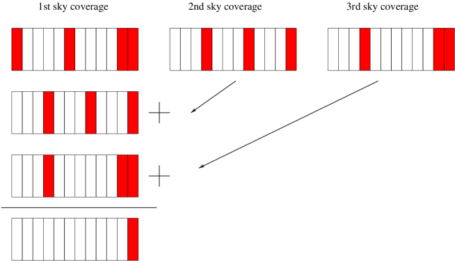
Figure 1: Schematic representation of the MC approach used here to simulate lost TM. The grey blocks represent portions of TM that is lost during the mission. The three sky coverages exactly overlap to obtain the final result in which only one block is effectively lost. Of course blocks that are “grey” in at least one sky coverage have intrinsically lower sensitivity in the final result.

We ran over 100,000 MC simulations to derive the probability distribution function of the lost TM. We assume two different mission durations implying 2 and 3 complete sky coverages. Each single sky coverage is composed of a total of 5,100 individual 1 hour scan circles (corresponding to $\simeq$ 7 months). Two total amounts of lost TM are considered: 5 and 2%.

In Table I we report results from our simulations respectively for 48 and 24 hours blocks of lost TM: $P(0)$ is the percentage of simulations with no loss of scan circles at all after coadding a given number of sky coverages (SC) while $P(\geq 1)$ is the percentage of simulations for which at least one scan circle is lost at the end of the coadding procedure. The other two columns report the mean and maximum number of scan circles lost in our 100,000 simulations.

Table 1: Results from 100,000 simulations with realistic loss of TM

TM Lost	TM Block	$P(0)$	$P(\geq 1)$	Mean #	Max #
5% - 2 SC	48	66.00	34.00	28.50$\pm$17.16	118
	24	38.23	61.77	18.19$\pm$11.64	78
5% - 3 SC	48	97.52	2.48	16.25$\pm$11.41	54
	24	94.35	5.65	8.64$\pm$5.89	37
2% - 2 SC	48	94.64	5.36	24.05$\pm$13.97	76
	24	87.45	12.55	12.85$\pm$7.29	46
2% - 3 SC	48	99.90	0.10	17.19$\pm$10.86	48
	24	99.68	0.32	7.56$\pm$5.06	20

While it is of course intuitive that a higher number of sky coverages decreases the probability of exact and partial overlap of portions of lost TM in each sky coverage, Table I clearly quantifies that the case with 5% of lost TM and with 3 sky coverages is considerable better than the case with only 2% of lost TM and 2 sky coverages.

In Figure 2 and Figure 3 we report the distribution of the number of scan circles lost after coadding sky coverages together, when considering loosing TM in 24 and 48 hours blocks respectively.

Figure 2: Distribution of number of scan circles lost - 24 hours sets

Figure 3: Distribution of number of scan circles lost - 48 hours sets

One interesting feature of these plots is that the cases with 3 sky coverages show a rapidly decreasing distribution with increasing number of scan circles lost while the cases with only 2 sky coverages have a much flatter distribution up to the dimension of the considered TM block. This means that in the latter cases there is almost the same probability of loosing a single scan circle or loosing 24 (48) or more scan circles. There is a clear sharp cut-off in these distribution functions at 24 (48) for the 24 (48) hours sets, respectively. Furthermore from a detailed study of the distribution of contiguous lost scan circles, we find that the probability of loosing sets of contiguous 24 (48) hours of scan circle is below 1% (0.1%) considering 5% of lost TM. These numbers fall futher down when considering 2% of lost TM.

2.2 Sky Fraction Lost

Another important aspect is the dimension of the lost TM projected into the sky when coadding the whole set of TM onto a sky map. This final step is somewhat dependent on the final resolution of the map to be created, i.e. the pixel size chosen for the map that is related to the beam width of the instrument collecting data. To evaluate the total sky fraction effectively lost, we first evaluate the probability distribution of the lost scan circles dimension. This goes, for the case of Planck, from the elementary dimension of a single ring of 2.5^′ up to a maximum value. Figures 4 and 5 show this probability distribution for the cases considered here.

Figure 4: Distribution of lost scan circles dimensions - 24 hours sets

Figure 5: Distribution of lost scan circles dimensions - 48 hours sets

As already seen for the distribution of number of scan circles lost, also in the distribution of dimensions we observe a flat distribution for the cases with 2 sky coverages while a rapidly decreasing distribution is present for 3 sky coverages. The same sharp cut-off observed in Figures 2 and 3 is clearly present in Figures 4 and 5 only for the 5% of lost TM and 2 sky coverages. The probability of loosing set of contiguous scan circles larger than the dimension of 24 (48) scan circles is practically zero.

It is now possible to evaluate the fraction of the sky that is left unobserved. This of course can be done only in a statistical sense.

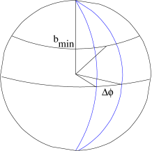
Figure 6: The equatorial displacement $\Delta\phi$ is the dimension of a given set of contiguous scan circles lost. The co-latitude $b_{\rm min}$ is the value at which the distance between the two meridians is comparable with pixel size.

In Figure 6, the two meridiands are the edges of the set of scan circles lost covering an angle $\Delta\phi$ along the equator. The value of $b_{\rm min}$ is derived from the map pixel size: it is the value of the co-latitude at which the distance between the edges in the figure is comparable with the pixel size. The “elementary” lost area is delimited by the edges, the equator and the isolatitude circle at $b_{\rm min}$. For evident symmetry reasons there are four of these “elementary” areas. The area of a lost scan chunk is then given by:

$$\Omega=4\times\int_{0}^{\Delta\phi}d\phi\int_{b_{\rm min}}^{\pi/2}d\theta{\rm sin}(\theta)$$ (1)

Knowing the distribution function $N(\Delta\phi)$ (see Figures 4 and 5), the total fraction of sky lost can be derived:

$$Area=\sum_{i}N(\Delta\phi)\Omega_{i}$$ (2)

where summation start from $\Delta\phi$ comparable with the pixel size, typically assumed to be $\sim 1/3$ of the beam FWHM.

In Table II we report the fraction of sky effectively lost for pixel size of 13.7^′ and 6.8^′ that are representative for a map at 30 GHz (FWHM=33.6^′) and at 70 GHz (FWHM = 22.3^′) that are the most critical Planck-LFI channels with respect to this issue. We report here only the case for 48 hours sets of lost TM.

Table 2: Summary of sky fraction lost for two different pixel sizes - 48 hours set

TM Lost	Pixel size [′]	Area [Sq. degress]	Fraction [%]
5% - 2 SC	13.7	88.62	0.21
5% - 3 SC	13.7	3.62	8.8 $\times 10^{-3}$
2% - 2 SC	13.7	12.14	0.029
2% - 3 SC	13.7	0.13	3.1 $\times 10^{-4}$
5% - 2 SC	6.8	91.40	0.22
5% - 3 SC	6.8	3.87	9.4 $\times 10^{-3}$
2% - 2 SC	6.8	12.54	0.030
2% - 3 SC	6.8	0.14	3.3 $\times 10^{-4}$

Inspection of Table II shows that the area of lost sky depends on the pixel size of the map only weakly: when the pixel size decreases by a half the area of the lost sky increases only by a tiny fraction. The improvement represented by the case of 5% lost TM with 3 sky coverages with respect to the case with 2% lost TM but only 2 sky coverages is quite clear.

3 Discussion and Conclusions

We have derived through MC simulations the probability of loosing TM packets for a space-borne instrument performing a full-sky survey.

Of course, it is obvious that the best results for a sky coverage in terms of completeness are obtained when the largest fraction of TM is retained and the number of repeated full sky observations is increased. However, our analysis clearly shows that it is better to cover the sky more times with a lower fraction of TM retained than less times with a higher TM fraction.

In this respect we note that the 5 year full sky mission GAIA assumes 5 repetitions of essentially the same scanning strategy, year by year. Even in the most conservative case in which a given sky region is observed only one time per year, and considering that: i) the total capacity of the on-board data recorder is about 1 day, ii) one day is also the time scale for the $\sim 1^{\circ}$ re-pointing of the symmetry axis of GAIA scanning strategy, and iii) the field of view is about $1^{\circ}\times 1^{\circ}$ (not far from the Planck beam size at lower frequencies), we have a probability to loose a given sky region with 95% of guaranteed TM is less that $3\times 10^{-5}$%. This is another remarkable example in which the increase in the number of full sky surveys of the mission allows to significantly reduce the probability of loosing scientific information.

In a space mission, trading off the pergentage of guaranteed TM delivered to the ground versus number of full sky surveys has an impact in terms of costs: the setup needed to guarantee a higher TM fraction may imply more ground stations to follow the satellite and more ground personnel. Cost-wise, it could be preferable to make an extension of mission time that implies, e.g. in the case of Planck, only another seven months of operations. In any case, a careful costs-to-benefits analysis needs to be carried out.

Acknowledgements

It is a pleasure to thank Floor Van Leeuwen, Michael Perryman and José-Luis Pellon-Bailon for useful discussions on the GAIA scanning strategy. We warmly thank the referee for constructive comments.

References

- [1] \harvarditemBennett et al.1996bennett96 Bennett, C. L., et al., Amer. Astron. Soc. Meet., 88.05, 1996
- [2] \harvarditemBurigana et al.2001buri01 Burigana, C., Butler, C., Mandolesi, N., Planck-LFI: Pointing Accuracy Requirements, PL-LFI-PST-TN-023, 2001
- [3] \harvarditemMandolesi et al.1998mando00 Mandolesi, N., et al., Planck-LFI, A Proposal Submitted to the ESA, 1998
- [4] \harvarditemPerryman et al.2001perry01 Perryman, M. A. C., et al., A&A, 369, 339 (2001)
- [5] \harvarditemPilbratt2000pilb00 Pilbratt, G. L., “The Herschel Mission, Scientific Objectives and this meeting”, in Proceeding of the Symposium on 12-15 December 2000, held in Toledo, Spain, ESA SP-460, 13
- [6] \harvarditemPuget et al.1998puget00 Puget, J. L., et al., Planck-HFI, A Proposal Submitted to the ESA, 1998
- [7] \harvarditemTauber2000tauber00 Tauber, J. A., “The Planck Mission”, in The Extragalactic Infrared Background and its Cosmological Implications, Proceedings of the IAU Symposium, Vol. 204, 2000, M. Harwit and M. Hauser, eds.
- [8]