Complex C: A Low-Metallicity High-Velocity Cloud Plunging into the Milky Way

Abstract

We present evidence that high-velocity cloud (HVC) Complex C is a low-metallicity gas cloud that is plunging toward the disk and beginning to interact with the ambient gas that surrounds the Milky Way. This evidence begins with a new high-resolution (7 km s^-1 FWHM) echelle spectrum of 3C 351 obtained with the Space Telescope Imaging Spectrograph (STIS). 3C 351 lies behind the low-latitude edge of Complex C, and the new spectrum provides accurate measurements of O I, Si II, Al II, Fe II, and Si III absorption lines at the velocity of Complex C; N I, S II, Si IV, and C IV are not detected at $3\sigma$ significance in Complex C proper. However, Si IV and C IV as well as O I, Al II, Si II and Si III absorption lines are clearly present at somewhat higher velocities associated with a “high-velocity ridge” (HVR) of 21cm emission. This high-velocity ridge has a similar morphology to, and is roughly centered on, Complex C proper. The similarity of the absorption lines ratios in the HVR and Complex C suggest that these structures are intimately related. In Complex C proper we find [O/H] = $-0.76^{+0.23}_{-0.21}$. For other species, the measured column densities indicate that ionization corrections are important. We use collisional and photoionization models to derive ionization corrections; in both models we find that the overall metallicity $Z=0.1-0.3Z_{\odot}$ in Complex C proper, but nitrogen must be underabundant. The iron abundance indicates that the Complex C contains very little dust. The size and density implied by the ionization models indicate that the absorbing gas is not gravitationally confined. The gas could be pressure-confined by an external medium, but alternatively we may be viewing the leading edge of the HVC, which is ablating and dissipating as it plunges into the Milky Way. O VI column densities observed with FUSE toward nine QSOs/AGNs behind Complex C support this conclusion: $N$(O VI) is highest near 3C 351, and the O VI/H I ratio increases substantially with decreasing latitude, suggesting that the lower-latitude portion of the cloud is interacting more vigorously with the Galaxy. The other sight lines through Complex C show some dispersion in metallicity, but with the current uncertainties, the measurements are consistent with a constant metallicity throughout the HVC. However, all of the Complex C sight lines require significant nitrogen underabundances. Finally, we compare the 3C 351 data to high-resolution STIS observations of the nearby QSO H1821+643 to search for evidence of outflowing Galactic fountain gas that could be mixing with Complex C. We find that the intermediate-velocity gas detected toward 3C 351 and H1821+643 has a higher metallicity and may well be a fountain/chimney outflow from the Perseus spiral arm. However, the results for the higher-velocity gas are inconclusive: the HVC detected toward H1821+643 near the velocity of Complex C could have a similar metallicity to the 3C 351 gas, or it could have a significantly higher $Z$, depending on the poorly constrained ionization correction.

1 Introduction

The Galactic high-velocity clouds (HVCs), gas clouds detected via 21 cm emission or UV/optical absorption at velocities that deviate substantially from normal Galactic rotation (Wakker & van Woerden 1997), have potentially important implications regarding the structure and evolution of the Galaxy and Local Group. For example, if the HVCs provide a sufficient quantity of infalling low-metallicity gas, they can alleviate the G-dwarf problem, the long-standing discrepancy between the observed metallicity distribution of G-dwarf stars and theoretical expectations (e.g., Larson 1972; Tosi 1988; Wakker et al. 1999; Gibson et al. 2002). The HVCs may have important cosmological implications as well. Hierarchical models of galaxy formation within the cold dark matter framework predict many more dwarf satellite galaxies within the Local Group than have been detected/identified (e.g., Klypin et al. 1999; Moore et al. 1999). A variety of solutions to this problem have been proposed, including the possibility that the HVCs are the missing dwarfs which, for some reason, have not formed readily detectable stars (e.g., Blitz et al. 1999; Klypin et al. 1999; Gibson et al. 2002).

However, the nature of most high-velocity gas is still poorly understood, mainly because the cloud distances are highly uncertain. Some of the HVCs are clearly material stripped out of the Magellanic Clouds, the “Magellanic Stream” (Mathewson, Cleary, & Murray 1974; Putman et al. 1998; Lockman et al. 2002), and some high-velocity absorption lines observed towards disk stars are most likely related to the interaction between stars/supernovae and the ISM (e.g., Cowie, Songaila, & York 1979; Trapero et al. 1996; Jenkins et al. 1998, 2000; Welty et al. 1999; Tripp et al. 2002). Apart from these clouds, direct distance constraints are scarce and difficult to obtain (Wakker 2001), and consequently a variety of HVC models remain viable. The HVCs may have a galactic origin such as the Galactic fountain (Shapiro & Field 1976; Bregman 1980), or they may be extragalactic (e.g., Oort 1970; Blitz et al. 1999; Braun & Burton 1999).

Given the difficulty of direct distance measurements, it is important to explore other constraints on the nature of these objects. For example, constraints on the distribution and size of the HVCs can be derived from studies of other galaxy groups using either QSO absorption line statistics (Charlton, Churchill, & Rigby 2000) or surveys for redshifted 21 cm emission (Zwaan & Briggs 2000; Zwaan 2001; Braun & Burton 2001; Pisano & Wilcots 2003). For the Milky Way HVCs, it has been suggested that the H$\alpha$ emission from the clouds constrains their distances (e.g., Bland-Hawthorn et al. 1998). If the gas is photoionized by UV flux escaping from the Galaxy, then nearby clouds should be substantially brighter in H$\alpha$ than distant HVCs. H$\alpha$ emission has in fact been detected from a variety of HVCs (e.g., Weiner & Williams 1996; Tufte et al. 1998, 2002; Weiner, Vogel, & Williams 2002), and detailed photoionization models place the clouds roughly 5 $-$ 50 kpc away based on the observed H$\alpha$ intensities (Weiner et al. 2002; Bland-Hawthorn & Maloney 2002). However, several observations cloud the interpretation of H$\alpha$ intensities. First, the Magellanic Stream, which has an independently constrained distance, is much brighter in H$\alpha$ than predicted by the photoionization models (Weiner et al. 2002; Bland-Hawthorn & Maloney 2002). Second, the Magellanic Stream H$\alpha$ emission is spatially variable (see Figure 1 in Weiner et al. 2002), also contrary to the predictions of the photoionization models. Finally, O VI absorption has been detected in a substantial fraction of the HVCs (Sembach et al. 2000, 2002; Wakker et al. 2002). While O VI can be produced by photoionization in large, low-density intergalactic gas clouds (e.g., Tripp & Savage 2000; Tripp et al. 2001), the O VI in HVCs is almost certainly collisionally ionized (the cloud sizes required by photoionization models are excessive for HVCs, see Sembach et al. 2002). These observations suggest that collisional processes play an important role in the ionization of HVCs and the production of H$\alpha$ emission. The interaction of the rapidly moving clouds with ambient magnetic fields may create instabilities that also play a role in the gas ionization and production of H$\alpha$ emission (Konz et al. 2001). For these reasons, H$\alpha$ distance constraints from photoionization models may need to be revisited.

Ultraviolet absorption lines in the spectra of background quasars and active galactic nuclei (AGNs) provide another sensitive probe for the study of Galactic (as well as extragalactic) HVCs. UV absorption lines provide detailed information on abundances and physical conditions in the gas, and this in turn can be compared to predictions of various models. For example, it is expected that Galactic fountain gas would have a substantially higher metallicity than infalling extragalactic gas or gas stripped from a satellite galaxy. Relative metal abundance patterns may also provide insights on the enrichment history of the HVCs; if the gas is relatively pristine, overabundances of $\alpha$ elements or underabundances of nitrogen might be observed, as seen in low-metallicity stars (McWilliam 1997) and H II regions (Vila-Costas & Edmunds 1993; Henry, Edmunds, & Köppen 2000).

In this paper we use the absorption line technique to explore the nature of HVC Complex C, a large HVC (roughly 20${}^{\circ}\times 90^{\circ}$) that is at least $\sim$5 kpc away (van Woerden et al. 1999). A number of Complex C abundance measurements have been published for a variety of species ranging from [N/H] = $-1.94$ to [Fe/H] = $-0.3$ (Bowen, Blades, & Pettini 1995; Wakker et al. 1999; Murphy et al. 2000; Richter et al. 2001; Gibson et al. 2001; Collins et al. 2002). However, some of these abundances may be confused by ionization effects. Species such as S II or Fe II can arise in ionized as well as neutral gas leading to overestimates of [S/H] or [Fe/H] if no ionization correction is applied, while other species such as N I can be more readily ionized than H I leading to underestimation of the elemental abundance. The most robust species for constraining the metallicity of HVCs is O I. Like sulfur, oxygen is only lightly depleted by dust grains (see §6.2.1 in Moos et al. 2002, and references therein), but more importantly, the ionization potential of O I is nearly identical to that of H I, and O I is strongly locked to H I by resonant charge exchange (Field & Steigman 1971). Consequently, oxygen abundances based on O I and H I are relatively impervious to ionization effects (unless the gas is quite substantially ionized).

Richter et al. (2001) have presented the first measurement of [O/H] in Complex C using spectra of PG1259+593 obtained with the Space Telescope Imaging Spectrograph (STIS) and the Far Ultraviolet Spectroscopic Explorer (FUSE); they find [O/H] = $-1.03^{+0.37}_{-0.31}$. Notably, Richter et al. also report that nitrogen is highly underabundant (by $\sim$ 1 dex compared to oxygen), and the $\alpha$ elements are marginally overabundant compared to iron. These results suggest that Complex C is a relatively pristine extragalactic cloud plunging into the Galaxy for the first time. This notion has been challenged by Gibson et al. (2001), who have observed S II in several directions through Complex C and find evidence of spatial variability of the sulfur abundance. Sulfur abundances derived from S II alone are prone to ionization effects, as noted, but recently Collins, Shull, & Giroux (2003) have also reported variable metallicity in Complex C based on oxygen measurements.

Here we present new constraints on the metallicity as well as the physical conditions, structure, and nature of high-velocity cloud Complex C from UV absorption lines. Our analysis is mainly based on high-resolution echelle spectroscopy of 3C 351 obtained with STIS, but we make use of high-resolution observations of nearby sight lines to augment the results with spatial information, e.g., on the transverse extent of the absorbing gas. We also briefly discuss intermediate-velocity gas in the 3C 351 direction. The paper is organized as follows: We begin with a summary of 21cm emission observations of high-velocity gas in the direction of 3C 351 (§2), followed by a brief summary of the STIS observations (§3) and the absorption line measurements (§4). We then argue that ionization corrections are likely to be important for these clouds, and we employ collisional and photoionization models to constrain their abundances (§5). The abundances indicate that Complex C and the intermediate-velocity gas likely have different origins; we suggest that Complex C is an infalling, low-metallicity cloud while the IVC is outflowing gas from the Perseus spiral arm. In the discussion of our measurements, we consider the implications of the density and size of the absorbing gas derived from the ionization models including the confinement of the gas (§6.1), and we compare 3C 351 to other nearby sight lines in the vicinity of Complex C (§6.2). We find evidence that the lower latitude portion of Complex C is more affected by interactions with the ambient medium that the higher latitude region of the cloud. We summarize our conclusions in §7. Throughout this paper we present spectra and velocities relative to the Local Standard of Rest (LSR).

2 High-Velocity Clouds Toward 3C 351

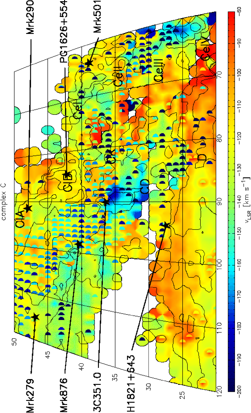
Figure 1: Map of HVC Complex C 21 cm emission, from Hulsbosch & Wakker (1988), in Galactic coordinates (longitude increases from right to left along the x-axis). This map is centered on the sight line to 3C 351 and shows only a portion of the cloud (for a map of the entire HVC, see Figure 6 in Wakker 2001). Emission from high-velocity gas in the Outer Arm is also evident in this map closer to the plane; at $l>90^{\circ}$ and $b<30^{\circ}$, the high-velocity emission is dominated by the Outer Arm. At lower longitudes the distinction is less clear; the line from $(l,b)=(70,25)$ to (88,29) roughly delineates these structures. LSR velocities are indicated by color using the scale at the bottom of the figure, and the contours show brightness temperatures of 0.05, 0.4, and 1.0 K. The half-circles show the high-velocity ridge at $v_{\rm LSR}\approx-200$ km s^-1; this higher velocity feature is clearly detected in absorption toward 3C351 (see text and Figures 6-8). The emission cores CIA,CIB, CeI-CeIV, CK, CD, and D are also labeled along with other extragalactic sight lines of interest discussed in this paper.

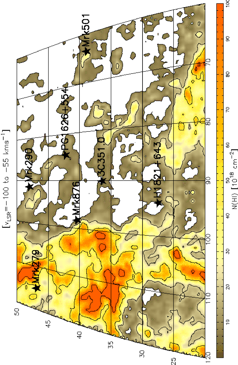
Figure 2: Map of 21 cm emission from intermediate-velocity gas in the vicinity of 3C 351 from the Leiden-Dwingeloo survey including the following velocity range: $-100\leq v_{\rm LSR}\leq-55$ km s^-1. Emission in this velocity range is dominated by the “IV Arch” at $l\gtrsim 98^{\circ}$; emission at lower latitudes may be associated with Complex K (see §4.24 and §4.27, respectively, in Wakker 2001) or the Perseus Arm (see text, § 6.2.3).

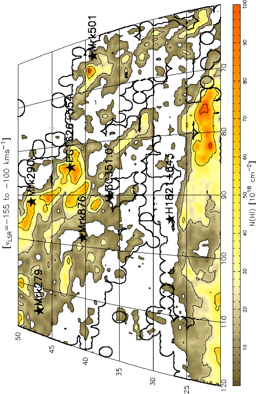
Figure 3: Partial map of Complex C 21 cm emission as in Figure 1, but based on data from the Leiden-Dwingeloo Survey (Hartmann & Burton 1997). Emission at $b\lesssim 27^{\circ}$ is mainly from the Outer Arm; higher-latitude emission is associated with Complex C. In this figure, colors indicate the H I column density as shown by the scale at the bottom, integrated from $v_{\rm LSR}=-155$ to $-100$ km s^-1. The lowest contour from the LDS data corresponds to the $3\sigma$ limit of $\sim 5\times 10^{18}$ cm^-2. The thick line indicates the $N$(H I) = $2\times 10^{18}$ cm^-2 contour from the Hulsbosch & Wakker map shown in Figure 1.

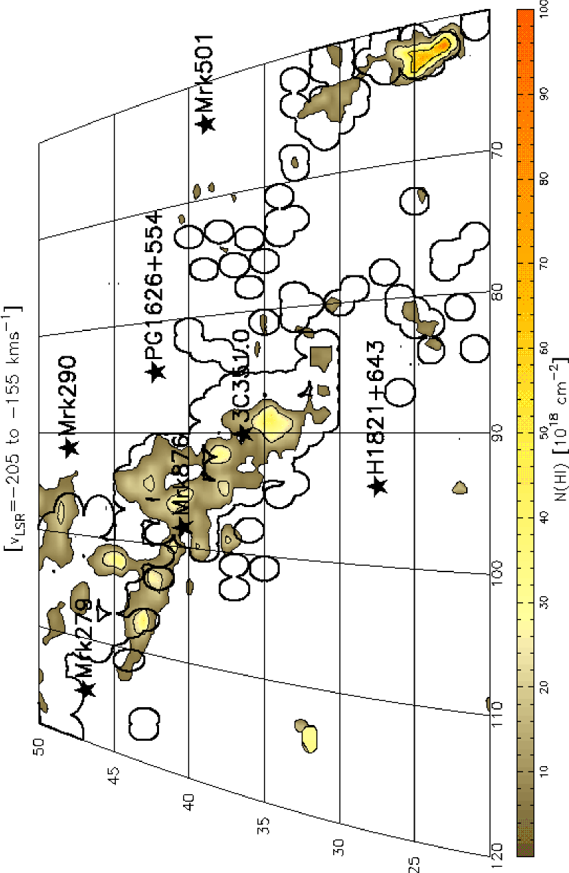
Figure 4: Map of 21 cm emission from the “High-Velocity Ridge” (see text) from the Leiden-Dwingeloo survey. This figure is identical to Figure 3, except the emission is integrated over a different velocity range: $-205\leq v_{\rm LSR}\leq-155$ km s^-1.

The sight line to 3C 351 ($l=90.08^{\circ}$, $b=+36.38^{\circ}$) probes an intriguing region of the high-velocity sky. A portion of the Hulsbosch & Wakker (1988) 21 cm emission map of Complex C, centered on 3C 351, is shown in Figure 1. In this figure, the color scale shows the LSR gas velocity while the contours indicate brightness temperature. The lowest contour shown corresponds to $N$(H I) = $2\times 10^{18}$ cm^-2. Complex C shows several well-defined cores; the 3C 351 sight line is roughly equidistant in projection from the CIB, CD, and CK cores [see Wakker (2001, and references therein) for definitions of the cores and nomenclature]. CK has a lower velocity than most of Complex C and may be more closely associated with the intermediate-velocity cloud Complex K than the high-velocity Complex C cloud (see Wakker 2001 and Haffner, Reynolds, & Tufte 2001). Figure 2 shows the intermediate-velocity 21 cm sky in the vicinity of 3C 351. The map in Figure 2 plots H I column densities derived from the 21 cm Leiden-Dwingeloo Survey (LDS; Hartmann & Burton 1997) integrated over $-100\leq v_{\rm LSR}\leq-55$ km s^-1. At $l\gtrsim 100^{\circ}$, the intermediate-velocity sky is dominated by the “IV Arch”, but at lower latitudes it is unclear whether the emission is associated with the IV Arch, Complex K, or a lower-velocity region of Complex C (see Wakker 2001). We provide evidence below that the CK IVC and Complex C proper have different origins (§§5.4,6). We shall refer to the 3C 351 intermediate-velocity absorption system as C/K hereafter and Complex C proper ($v_{\rm LSR}\approx-130$ km s^-1) as simply Complex C.

A notable feature of Complex C is the presence of 21 cm emission at substantially higher velocities ($v_{\rm LSR}\leq-170$ km s^-1) along the central ridge of the cloud superimposed on the main HVC emission ($-155\lesssim v_{\rm LSR}\lesssim-80$ km s^-1). The higher velocity emission is indicated with half-circles in Figure 1 (see also Figure 6 in Wakker 2001). The nature of the higher velocity component is not entirely clear, but it has a similar morphology to the lower velocity Complex C gas, and it is centered on Complex C. For convenience, we refer to this cloud as the “high-velocity ridge” (HVR) in this paper. A variety of UV absorption lines are detected from the high-velocity ridge in the 3C 351 spectrum as well as Complex C, and unlike C vs. C/K, the UV absorption lines provide evidence that the HV ridge and Complex C are closely related (see below).

The H I column densities in Complex C and the high-velocity ridge are shown in Figures 3 and 4, respectively. Figures 3-4 show 21 cm emission maps from the LDS integrated over $-155\leq v_{\rm LSR}\leq-100$ km s^-1  (Complex C proper) and $-205\leq v_{\rm LSR}\leq-170$ km s^-1 (high-velocity ridge). In these figures, the color scale and thin contours reflect $N$(H I) according to the scale at the bottom. The last thin contour is drawn at the 3$\sigma$ limit of the LDS, $N$(H I) = $5\times 10^{18}$ cm^-2. The thick line shows the $2\times 10^{18}$ cm^-2 contour from the more sensitive Hulsbosch & Wakker map in Figure 1 integrated over the same velocity range. Much of the high-velocity emission detected closer to the plane in Figures 1-3 is mainly associated with the Outer Arm and the warp of the outer Milky Way (Wakker 2001, and references therein).

A potentially serious source of systematic error in HVC abundance measurements is the large beam of the 21 cm observations usually used to estimate $N$(H I). The large radio beam may dilute the HVC 21 cm emission, or it may show emission from gas which is in the radio beam but is not present along the pencil beam to the UV source. Comparisons of $N$(H I) measurements from different radio telescopes (with different beam sizes) indicate that the 10’ Effelsberg beam is often sufficiently small to provide a reliable H I column density (Wakker et al. 2001), but there are cases where even the Effelsberg beam is too large (e.g., Mrk 205, see Wakker 2001). Therefore it is worthwhile to review the available $N$(H I) measurements for the 3C 351 HVCs. The HVC 21 cm emission profiles in the direction of 3C 351 observed with the NRAO 43m telescope (Murphy, Sembach, & Lockman 2002) and the Effelsberg 100m telescope (Wakker et al. 2001) are shown in Figure 5. H I column densities in the 3C 351 HVCs derived from these data are summarized in Table 1 along with $N$(H I) from the LDS data. The uncertainties listed in Table 1 are statistical errors only. Wakker et al. (2001) note that the systematic uncertainties in the 3C 351 H I column densities are likely much larger than the statistical errors: they estimate that systematic errors lead to an uncertainty of $\sim 1.5\times 10^{18}$ cm^-2 in $N$(H I). With this uncertainty, the $N$(H I) measurements in Table 1 for Complex C are in reasonable agreement. For Complex C, we adopt $N$(H I) from the smallest-beam observation (Effelsberg), but with the larger systematic uncertainty reported by Wakker et al., i.e., $N$(H I) = $(4.2\pm 1.5)\times 10^{18}$ cm^-2. However, while both Complex C proper and the high-velocity ridge are apparent in the NRAO and LDS data, only Complex C is clearly detected in the Effelsberg observation. This suggests that the observations with larger beams are picking up emission which is not present along the pencil beam to 3C 351. Consequently, we take the NRAO Green Bank $N$(H I) as an upper limit for the high-velocity ridge, and we derive lower limits on the HV ridge abundances below. Similarly, the H I column for Complex C/K is highly uncertain given the systematic uncertainty above, and we can only place lower limits on the metallicity of this IVC. However, these lower limits will turn out to be useful (§§5.3,5.4).

Figure 5: H I 21 cm emission profiles in the direction of 3C 351, recorded with (a) the NRAO 43m telescope (Murphy, Sembach, & Lockman 2002), and (b) the Effelsberg 100m telescope (Wakker et al. 2001). Brightness temperature is plotted vs. LSR velocity. Complex C proper and the high-velocity ridge are marked along with the intermediate-velocity cloud Complex C/K. H I column densities derived from these data are listed in Table 1.

Table 1: Intermediate-Velocity and High-Velocity Cloud H I Column Densities toward 3C 351

	Effelsberg 100m (10′ beam)		Green Bank 43m (21′ beam)		Dwingeloo 25m (35′ beam)
High-Velocity Cloud	$v_{\rm LSR}$	$N$(H I)	$v_{\rm LSR}$	$N$(H I)	$v_{\rm LSR}$	$N$(H I)
	(km s-1)	($10^{18}$ cm-2)	(km s-1)	($10^{18}$ cm-2)	(km s-1)	($10^{18}$ cm-2)
High-velocity ridge	$\cdots$	$\cdots$	$-182.2$	4.19	$-191$	$4.5\pm 0.9$
Complex C (proper)	$-129$	$4.2\pm 0.3$	$-128.2$	6.01	$-126$	$4.5\pm 0.6$
Complex C/K	$-89$	$1.3\pm 0.2$	$-83.0$	4.08	$-69$	$4.0\pm 0.5$

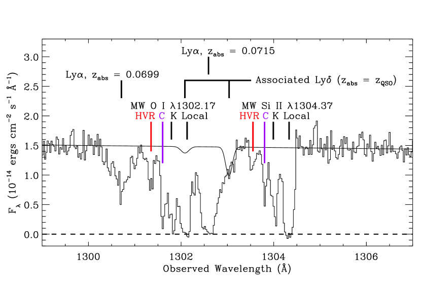
Figure 6: Portion of the FUV spectrum of 3C 351 obtained with STIS in the E140M echelle mode (FWHM $\approx$ 7 km s^-1) plotted versus observed wavelength. For display purposes, the spectrum has been binned (2 pixels into 1) in this figure (all other figures, as well as the line measurements, make use of the full resolution, unbinned spectrum). This region of the spectrum shows the absorption profiles of the O I $\lambda$1302.2 and Si II $\lambda$1304.4 lines due to the ISM of the Milky Way as well as several extragalactic absorption lines. Four main components are readily apparent in the Galactic O I and Si II profiles; these are indicated with tick marks immediately above the spectrum. We are mainly interested in the high-velocity absorption lines associated with Complex C and the “high-velocity ridge” (HVR, see §2), which are marked with longer tick marks. Absorption arising in the intermediate-velocity cloud Complex C/K and local gas is also identified with short ticks. The thin solid line indicates the fitted continuum with the predicted Ly$\delta$ lines due to the associated absorption systems at $z_{\rm abs}$ = 0.3709 and 0.3719 superimposed (see Yuan et al. 2002). The other extragalactic lines in this wavelength range are identified as Ly$\alpha$ at $z_{\rm abs}$ = 0.0699 and 0.0715 (see text for further details).

Figure 7: Effelsberg 21 cm emission profile (top left panel) and selected UV absorption line profiles of Milky Way lines detected toward 3C 351, plotted versus Local Standard-of-Rest (LSR) velocity. Brightness temperature is plotted in the top left panel, and observed flux is shown in the other panels. Dashed lines show the fitted continua and dotted lines mark the flux zero level. Absorption lines due to Complex C and the “High-Velocity Ridge” (HVR, see text) are indicated with tick marks. Unrelated absorption features are also marked ($\times$).

3 STIS Echelle Spectroscopy

We now turn to the UV absorption line data. The STIS observations of 3C 351 are fully described in §2 of Yuan et al. (2002). Briefly, the QSO was observed with the E140M echelle mode with the $0\farcs 2\times 0\farcs 06$ slit; this mode provides 7 km s^-1 resolution (FWHM) and covers the 1150 $-$ 1710 Å range with only a few gaps between orders at the longest wavelengths (see Woodgate et al. 1998 and Kimble et al. 1998 for further details). The data were reduced following standard procedures with software developed by the STIS Investigation Definition Team. Scattered light was removed using the procedure developed by the STIS Team (Bowers et al. 1998), which corrects for echelle scatter as well as other sources of scattered light.

A sample of the final spectrum is shown in Figure 6. This somewhat complicated portion of the spectrum shows the absorption profiles of the important Milky Way O I $\lambda$1302.2 and Si II $\lambda$1304.4 profiles as well as several extragalactic absorption lines. Absorption profiles of several species of interest are plotted versus LSR velocity in Figure 7 along with the H I 21 cm emission observed in the direction of 3C 351 by Wakker et al. (2001) with the 100 m Effelsberg telescope. The UV absorption lines show four distinct components. The two highest-velocity components at $v_{\rm LSR}$ = $-128$ and $-190$ km s^-1 are close to the observed 21 cm velocities of Complex C and the high-velocity ridge. Similarly, the UV lines at $v_{\rm LSR}$ $\approx-82$ km s^-1 are close to the velocity of IVC C/K. Analysis of the Complex C/K absorption lines is complicated by substantial blending with adjacent components. Nevertheless, the data indicate that IVC C/K has a higher metallicity than HVC Complex C (§5.4).

In this paper, we are primarily interested in Complex C and the high-velocity ridge. However, absorption from other Galactic and extragalactic clouds can introduce systematic errors that must be considered. For example, 3C 351 has a dramatic “associated” absorption system (i.e., $z_{\rm abs}\approx z_{\rm QSO}$) that affects the spectrum near the N V, O VI, and Lyman series lines at the redshift of the QSO (Yuan et al. 2002, and references therein). The associated Ly$\delta$ lines at $z_{\rm abs}$ = 0.3709 and 0.3719 fall near the Galactic O I $\lambda 1302.2$ profile, which is a crucial profile for our analysis. We can predict the strength of these contaminating Ly$\delta$ lines based on fits to the other Lyman series lines in the STIS spectrum from Yuan et al. (2002). The thin solid line in Figure 6 shows the predicted Ly$\delta$ lines superimposed on the fitted continuum. Fortunately, as can be seen from Figure 6, these associated Ly$\delta$ lines have no impact on the high-velocity O I lines of primary interest. The nearby Ly$\alpha$ lines at $z_{\rm abs}$ = 0.0715 and particularly 0.0699 could be a more serious source of contamination than the associated Ly$\delta$ lines. These Ly$\alpha$ lines appear to be mostly separated from the Milky Way O I and Si II profiles, but since Ly$\alpha$ lines are clustered on velocity scales of a few hundred km s^-1 (Penton et al. 2000), it remains possible that unseen Ly$\alpha$ lines clustered around the strong $z_{\rm abs}$ = 0.0699 and 0.0715 absorbers affect the Galactic O I and/or Si II profiles in Figure 6. However, a detailed comparison of the Milky Way profiles in the following section indicates that there is little or no contamination present in the O I and Si II lines.

The Galactic Si II $\lambda 1193.3$ transition is badly blended with C III $\lambda 977.0$ absorption from a Lyman limit system at $z_{\rm abs}$ = 0.2210, so we do not use this transition for the HVC analysis. Also, the Milky Way Si II $\lambda 1190.4$ and S III $\lambda 1190.2$ transitions are highly blended, and we do not trust information from either of these lines. Finally, we note that the Galactic Si II $\lambda 1260.4$ and C II $\lambda 1334.5$ transitions are severely saturated and consequently do not provide useful constraints.

4 Absorption Line Measurements

To measure the line column densities and to assess the impact of unresolved saturation on the absorption lines of interest, we mainly rely on the apparent column density technique (Savage & Sembach 1991), but some supporting measurements are also derived from Voigt profile fitting, using the software of Fitzpatrick & Spitzer (1997) with the line spread functions from the STIS Instrument Handbook (Leitherer et al. 2001). The apparent column density is constructed using the following expression,

$$N_{\rm a}(v)\ =\ (m_{\rm e}c/\pi e^{2})(f\lambda)^{-1}\tau_{\rm a}(v)\ =\ 3.768\times 10^{14}(f\lambda)^{-1}{\rm ln}[I_{\rm c}(v)/I(v)].$$ (1)

This provides the instrumentally broadened column density per unit velocity [in atoms cm^-2 (km s^-1)^-1], where $f$ is the transition oscillator strength, $\lambda$ is the transition wavelength (the numerical coefficient is for $\lambda$ in Å), $I(v)$ is the observed line intensity and $I_{\rm c}(v)$ is the estimated continuum intensity at velocity $v$. By comparing two or more resonance lines of a given species with adequately different $f\lambda$ values, the profiles can be checked for unresolved saturation and a correction can, in some cases, be applied (Jenkins 1996). If the $N_{\rm a}(v)$ profiles of the resonance lines are in good agreement, then the lines are not affected by unresolved saturation, and the profiles can be integrated to obtain the total column, $N_{\rm tot}=\int N_{\rm a}(v)dv.$

High-velocity absorption line equivalent widths and apparent column densities, integrated across the velocity ranges that delimit Complex C proper and the high-velocity ridge, are summarized in Table 2. These measurements were made using the methods of Sembach & Savage (1992) and include continuum placement uncertainty and a 2% flux zero point uncertainty in addition to the statistical uncertainties. Column densites of well-detected species determined from Voigt profile fitting ($N_{\rm pf}$) are also listed. Equivalent widths and column densities for the intermediate-velocity C/K cloud are provided in Table 3. The abundance measurements presented in the last two columns of Tables 2-3 are discussed in §5.

Table 2: High-Velocity Absorption Lines toward 3C 351: Complex C and the High-Velocity Ridge

Species	$\lambda_{0}$	$f$	Cloud	$<v>$	$W_{\lambda}$	log $N_{\rm a}$	log $N_{\rm pf}$	[Xi/H I]	[X/H]
	(Å)			(km s-1)	(mÅ)
O I	1302.17	0.0519	Complex C	$-128\pm 1$	115.1$\pm$4.9	14.45$\pm$0.04	14.63${}^{+0.10}_{-0.14}$	$-0.73^{+0.23}_{-0.21}$	$-0.76^{+0.23}_{-0.21}$
			HV Ridge	$-190\pm 2$	81.8$\pm$8.1	14.12$\pm$0.05	14.17$\pm$0.04	$>-1.24$	$>-1.26$
N I	1199.55	0.130	Complex C	$-130\pm 3$	(24.6$\pm$10.8)	$<$13.44	$\cdots$	$<-1.11$	$<-1.37$
			HV Ridge	$\cdots$	(3.7$\pm$14.6)	$<$13.55	$\cdots$	$\cdots$	$\cdots$
Si II	1304.37	0.0917	Complex C	$-128\pm 1$	63.3$\pm$4.6	13.81$\pm$0.05	13.77$\pm$0.04	$-0.40^{+0.20}_{-0.14}$	$-0.73^{+0.20}_{-0.14}$
			HV Ridge	$-183\pm 5$	30.3$\pm$7.1	13.42${}^{+0.08}_{-0.12}$	13.50$\pm$0.05	$>-0.70$	$>-1.26$
	1526.71	0.132	Complex C	$-128\pm 1$	86.1$\pm$6.5	13.72$\pm$0.05	13.77$\pm$0.04	$-0.40^{+0.20}_{-0.14}$	$-0.73^{+0.20}_{-0.14}$
			HV Ridge	$-184\pm 3$	68.8$\pm$10.5	13.49${}^{+0.06}_{-0.08}$	13.50$\pm$0.05	$>-0.70$	$>-1.26$
Al II	1670.79	1.83	Complex C	$-127\pm 1$	105.0$\pm$6.9	12.57$\pm$0.04	12.56$\pm$0.05	$-0.52^{+0.21}_{-0.15}$	$-0.88^{+0.21}_{-0.15}$
			HV Ridge	$-182\pm 3$	70.1$\pm$11.6	12.30${}^{+0.06}_{-0.08}$	12.33$\pm$0.05	$>-0.79$	$>-1.36$
S II	1259.52	0.0166	Complex C	$-124\pm 6$	(12.0$\pm$5.6)	$\leq 14.0$	$\cdots$	$<0.05$	$<-0.31$
			HV Ridge	$\cdots$	(1.1$\pm$7.9)	$\leq 14.1$	$\cdots$	$\cdots$	$\cdots$
Fe II	1608.45	0.0580	Complex C	$-125\pm 2$	63.1$\pm$8.7	13.78${}^{+0.06}_{-0.08}$	13.88${}^{+0.14}_{-0.21}$	$-0.29^{+0.22}_{-0.17}$	$-0.54^{+0.22}_{-0.17}$
			HV Ridge	$\cdots$	(12.4$\pm$13.8)	$\leq 13.6$	$\cdots$	$\cdots$	$\cdots$
Si III	1206.50	1.67	Complex C	$-127\pm 2$	115.2$\pm$7.6	12.91$\pm$0.06	$\cdots$	$\cdots$	$\cdots$
			HV Ridge	$-189\pm 3$	196.0$\pm$12.5	$>13.07$	13.40$\pm$0.10	$\cdots$	$\cdots$
Si IV	1393.76	0.514	Complex C	$-118\pm 13$	(7.1$\pm$6.2)	$\leq 12.4$	$\cdots$	$\cdots$	$\cdots$
			HV Ridge	$-188\pm 4$	45.1$\pm$8.4	12.77${}^{+0.08}_{-0.09}$	12.79$\pm$0.07	$\cdots$	$\cdots$
C IV	1548.20	0.191	Complex C	$-120\pm 8$	(14.6$\pm$8.9)	$\leq 13.0$	$\cdots$	$\cdots$	$\cdots$
			HV Ridge	$-191\pm 3$	100.2$\pm$11.6	13.50$\pm$0.06	13.54${}^{+0.16}_{-0.26}$	$\cdots$	$\cdots$

Table 3: Intermediate-Velocity Absorption Lines toward 3C 351: Complex C/K

Species	$\lambda_{0}$	$<v>$	$W_{\lambda}$	log $N_{\rm a}$	log $N_{\rm pf}$	[Xi/H I]	[X/H]
	(Å)	(km s-1)	(mÅ)
O I	1302.17	$-82\pm 1$	180.6$\pm$5.4	$>14.66$	14.85${}^{+0.18}_{-0.15}$	$\geq-0.50$	$\geq-0.52$
N I	1199.55	$-83\pm 10$	66.5$\pm$13.5	13.63${}^{+0.10}_{-0.14}$	$\cdots$	$\geq-0.91$	$\geq-0.69$
Si II	1304.37	$-81\pm 1$	131.3$\pm$4.9	$>14.23$	14.35${}^{+0.13}_{-0.10}$	$\geq 0.20$	$\geq-0.52$
	1526.71	$-81\pm 1$	181.1$\pm$7.0	$>14.09$	14.35${}^{+0.13}_{-0.10}$	$\geq 0.20$	$\geq-0.52$
Al II	1670.79	$-82\pm 1$	191.1$\pm$7.2	12.88$\pm$0.04	$\sim 13.1$	$\geq-0.20$	$\geq-0.88$
S II	1259.52	$-86\pm 4$	26.1$\pm$6.2	14.10${}^{+0.10}_{-0.12}$	$\cdots$	$\geq 0.16$	$\geq-0.46$
Fe II	1608.45	$-84\pm 2$	79.9$\pm$10.2	13.91$\pm$0.07	13.86$\pm 0.10$	$\geq-0.15$	$\geq-0.64$
Si IV	1393.76	$-83\pm 2$	68.9$\pm$6.3	12.98$\pm$0.05	13.03$\pm 0.06$	$\cdots$	$\cdots$
C IV	1548.20	$-82\pm 1$	110.6$\pm$9.0	13.58$\pm$0.05	13.29$\pm 0.07$	$\cdots$	$\cdots$

As noted in §1, the most important species for metallicity measurements is O I. The only O I transition available in the direction of 3C 351 is the 1302.2 Å line. In the high-velocity ridge, $N$(O I) appears to be well-constrained from the 1302.2 Å  profile. In Complex C, on the other hand, the 1302.2 Å line does not go to zero flux in the core, but it is quite strong (see Figs. 6-7). Consequently, it is important to consider whether the Complex C O I column might be underestimated due to unresolved saturation. We believe that the O I line is not seriously saturated based on the following evidence. We first note that the Si II lines show no indications of unresolved saturation. Figure 8a compares the $N_{\rm a}(v)$ profiles of the 1304.4 and 1526.7 Å lines of Galactic Si II, transitions that differ in $f\lambda$ by 0.23 dex. These Si II $N_{\rm a}(v)$ profiles are in good agreement, which indicates that the lines are not significantly saturated. If O I is affected by unresolved saturation, then the O I $N_{\rm a}(v)$ profile should differ from the Si II $N_{\rm a}(v)$ profiles due to the underestimation of $N$(O I) in the saturated pixels. Figure 8b compares the O I apparent column density to a weighted composite Si II $N_{\rm a}(v)$ profile constructed from the 1304.4 and 1526.7 profiles following the procedure of Jenkins & Peimbert (1997), with the O I profile scaled down by a factor of five. From Figure 8b, we see that the O I and Si II profiles have very similar shapes. This suggests that there is little unresolved saturation within the O I profile. We notice from Table 2 that Voigt profile fitting gives a somewhat higher $N$(O I) than direct $N_{\rm a}(v)$ integration, although the O I columns from the two methods agree within the 1$\sigma$ uncertainties. This could reflect a small amount of saturation. To be conservative, we adopt the higher $N$(O I) value for our subsequent analysis. However, we will consider the lower O I column in our analysis, and we will find that our conclusions are essentially the same.

The comparison of the O I and Si II $N_{\rm a}(v)$ profiles in Figure 8b also indicates that there is little contamination of the O I lines from the nearby Ly$\alpha$ absorbers discussed in §3 and shown in Figure 6. Significant optical depth from such contamination would cause the O I and Si II profiles to have different shapes at velocities where the contamination occurs. The O I and Si II profiles have similar velocity structure, and moreover the O I/Si II column density ratio is very similar in Complex C and the high-velocity ridge. The Al II and Si II $N_{\rm a}(v)$ profiles are also remarkably alike, as shown in Figure 8d. The Fe II $N_{\rm a}(v)$ profile is compared to the composite Si II profile in Figure 8c. Fe II is clearly detected in Complex C, but the substantially greater noise limits comparisons of C and the HV ridge for this species. The similarity of the O I, Si II, and Al II profiles in Figure 8 would seem to suggest that the physical conditions and relative abundances in Complex C and the high-velocity ridge are roughly the same. However, the behavior of the higher ionization stages (Si IV and C IV) is entirely different in Complex C and the high-velocity ridge, as shown in in Figure 8e-f. Very little high-ion absorption is apparent in the velocity range of Complex C, but Si IV and C IV are clearly detected in the high-velocity ridge, with component structure similar to that of the lower ionization stages. The Si IV and C IV profiles therefore indicate that there is a important difference in the physical conditions of Complex C and the HV ridge. We discuss this issue further in the following section.

Figure 8: Apparent column density as a function of LSR velocity ($N_{\rm a}(v)$, see text § 4) of selected absorption lines detected in the high-velocity clouds in the direction of 3C 351. (a) $N_{\rm a}(v)$ profiles of the Si II transitions at 1304.4 Å (filled circles) and 1526.7 Å (open circles). The good agreement of these transitions indicates that the lines are not strongly affected by unresolved saturation. (b) O I $\lambda$1302.2 profile scaled by 0.2 (open squares) vs. a weighted composite Si II profile (histogram). (c) Fe II $\lambda$1608.5 profile (filled circles) vs. the composite Si II profile (histogram). (d) Al II $\lambda$1670.8 profiles scaled by 17.0 (open squares) vs. the composite Si II profile (histogram). (e) Si IV $\lambda$1393.8 profile scaled by 5.0 (filled circles) vs. the composite Si II profile (histogram). (f) C IV $\lambda$1548.2 profile (open squares) vs. the composite Si II profile (histogram).

Figure 8: continued

Figure 8: continued

5 Abundances and Ionization

We next consider the implications of the measurements presented above. We first argue that ionization corrections are important in the 3C 351 HVCs (§5.1). We then investigate the absolute and relative abundances in Complex C and the high-velocity ridge with the aid of ionization models (§§5.2$-$5.4).

5.1 Preliminary Remarks

In general, the logarithmic abundance of species X with respect to species Y is

$$\left[\frac{\rm X}{\rm Y}\right]={\rm log}\left(\frac{N({\rm X}^{i})}{N({\rm Y}^{i})}\right)+{\rm log}\left(\frac{f({\rm Y}^{i})}{f({\rm X}^{i})}\right)-{\rm log}\left(\frac{\rm X}{\rm Y}\right)_{\odot},$$ (2)

where $N({\rm X}^{i})$ and $f({\rm X}^{i})$ are the column density and ion fraction of the $i^{\rm th}$ ionization stage of species X (and likewise for Y), and (X/Y)_⊙ is the solar reference abundance. In many situations, the ionization correction $f({\rm Y}^{i})/f({\rm X}^{i})$ can be neglected, e.g., if $f({\rm Y}^{i})=f({\rm X}^{i})=1$. However, when we state that the “ionization correction is decreasing”, this does not indicate that the ionization correction is becoming negligible; this only indicates that $f({\rm Y}^{i})/f({\rm X}^{i})$ is decreasing. In this paper, to distinguish between measurements that have been corrected for ionization and those which have not, we adopt the following notation: uncorrected abundances are indicated by the observed ion, e.g., [Si II/H I], while measurements which have had an ionization correction applied are indicated without reference to a particular ion, e.g., [Si/H]. The penultimate columns of Tables 2-4 list the uncorrected abundances implied by our column density measurements. The last columns of these tables summarize the ionization-corrected abundances, using the ionization models described in the sections below. For the high-velocity ridge and IVC C/K, we list lower limits on the abundances because we only have upper limits on $N$(H I) for these components (see § 2). Ionization corrections can be a large source of uncertainty; we present examples below. The $N$(H I) measurements are often the other main source of uncertainty. We include our best estimates of the $N$(H I) uncertainty in our abundance error bars. However, systematic errors in $N$(H I) due to radio beam effects can be much larger than statistical errors, and these uncertainties can be difficult to assess.

If we neglect the ionization correction for the Complex C absorption lines toward 3C 351, we obtain highly discrepant results from neutral-gas tracers compared to species that can persist in ionized gas, i.e., the different ions imply significantly different metallicities. For example, we obtain [O I/H I] $=-0.7$ and [N I/H I] $\lesssim-1.1$ vs. [Si II/H I] $=-0.4$, [Fe II/H I] $=-0.3$, and [Al II/H I] = $-0.5$. If correct, these abundances would indicate a very unusual relative abundance pattern. It is more likely that these discrepancies indicate that ionization corrections are important for the 3C 351 sight line. These abundance discrepancies are larger than the uncertainties in the respective measurements, as shown in Figure 11. In this figure we plot relative abundance measurements or limits, with respect to Si II, for Complex C, the high-velocity ridge, and IVC C/K derived directly from the O I, N I, Fe II, Al II, and S II lines, i.e., without ionization corrections. We plot abundances relative to Si II because we do not have a robust $N$(H I) measurement in the high-velocity ridge or IVC C/K, and because Si II is the best-constrained species in Complex C. The abundances in Figure 11 are arranged according to ionization potential. Again, we see evidence of ionization effects in all three of these clouds: the neutral species O I and N I are significantly underabundant with respect to Si II while ionized-gas tracers (Fe II and Al II) are much closer to the solar pattern.

Figure 11: Logarithmic abundances, with respect to silicon, of O I, N I, Fe II, Al II, and S II in Complex C (filled circles), the high-velocity ridge (open squares), and the intermediate-velocity cloud C/K (open triangles) in the direction of 3C 351. The abundances in the outer arm component toward H1821+643 are also shown (open diamonds). The species are plotted in order of increasing ionization potential (shown in parentheses in eV below each element; the IP of Si II is 16.35 eV). No ionization corrections have been applied. The underabundances of O I and N I with respect to Si II suggest that ionization corrections are important.

5.2 Complex C Proper

5.2.1 Collisional Ionization

Can we reconcile the various abundances by applying ionization corrections? Since we have reasons to believe that collisional processes may be important (see §1), and in order to make our development more clear, we begin with a simplified picture where collisional ionization equilibrium applies, with no additional photoionization from an energetic radiation field (we will add photoionization in the next section). Figure 12 shows relevant column density ratios, as a function of temperature, derived from the equilibrium collisional ionization calculations of Sutherland & Dopita (1993) with solar reference abundances from Holweger (2001) and Grevesse et al. (1996). The observed ratios in Complex C are overplotted for comparison. We see that over the temperature range in which the O I/Si II ratio is reproduced (within 1$\sigma$), the model does not exactly match the other observed ratios; departures from solar relative abundances are required. Nitrogen, for example, must be made underabundant with respect to silicon by at least $0.5-0.7$ dex (an underabundance moves the model curves down in Figure 12). This may not be surprising since there is other evidence that nitrogen is underabundant in Complex C (Richter et al. 2001; Collins et al. 2003), and nucleosynthesis in low-metallicity gas can result in N underabundances (e.g., Henry et al. 2000). Similarly, Figure 12 indicates that aluminum must be underabundant if the gas is collisionally ionized and in equilibrium. Like nitrogen, Al could be underabundant, although much less so, due to nucleosynthesis effects since it is an odd-Z element, as observed in low-metallicity Galactic field stars (e.g., Lauroesch et al. 1996). An Al underabundance in the gas phase could alternatively be due to depletion by dust since aluminum is highly refractory (e.g., Jenkins 1987). However, this would be inconsistent with the iron abundance: Fe II should also be depleted in this case, but Figure 12 seems to require a slight Fe overabundance, by $\sim$0.2 dex, which leaves little room for dust depletion.

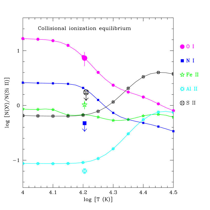
Figure 12: Column density ratios predicted in collisional ionization equilibrium vs. gas temperture, based on the calculations of Sutherland & Dopita (1993) with solar relative abundances from Holweger (2001) or Grevesse et al. (1996). Ratios of various species to $N$(Si II) are shown with small symbols according to the key on the right side. Observed ratios are plotted at log $T=4.2$ with larger symbols and 1$\sigma$ error bars. Arrows indicate 4$\sigma$ upper limits.

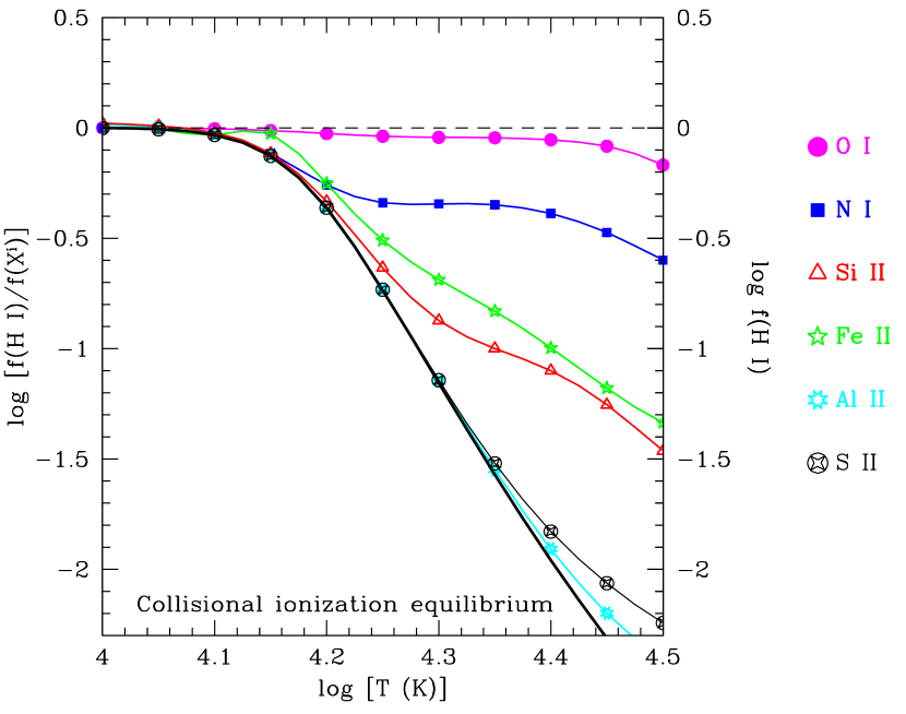
Figure 13: Ionization corrections for collisionally ionized gas in equilibrium from the calculations of Sutherland & Dopita (1993) vs. log $T$. As in Figure 12, the species corresponding to each curve is indicated by the key at the right. The H I ion fraction ($f$ = H I/H_total) is shown with a heavy black line using the scale on the right axis. The Al II and S II curves are very similar because over this temperature range, $f$(Al II) $\approx f$(S II) $\approx 1$, so the ionization correction is nearly equal to $f$(H I).

The only puzzling implication of Figure 12 is, in fact, the Fe overabundance. Nitrogen and Al underabundances would imply, at face value, that the gas is relatively pristine. However, in this case Fe should be underabundant as well since iron is thought to be mainly synthesized on longer timescales in Type Ia supernovae. We note the Fe II profile is the noisiest measurement among the detected lines (compare Figure 8c to the other panels in Fig. 8), and the observed Fe II/Si II ratio is only 2$\sigma$ above the model prediction at log $T\sim$ 4.2. The slight Fe overabundance may simply be a result of noise. In fact, we shall see below that when uncertainties in the reference abundances as well as the column density measurements are taken into account and ionization corrections are applied, the final abundances agree within 1$\sigma$, except nitrogen. However, it is clear that iron is not highly underabundant due to dust depletion or nucleosynthesis effects. We also note that Murphy et al. (2000) find a relatively high Fe II/H I ratio for Complex C in the direction of Mrk 876. For Figure 12, we assumed solar relative abundances. If we were to adopt overabundances of the $\alpha-$elements (O I, Si II, and S II) by $\sim$0.3 dex, on the grounds that such patterns are observed in low-metallicity stars (McWilliam 1997, and references therein), then we would have a substantial discrepancy between the observed and model Fe II columns.

For the calculation of abundances using equation 2, we present in Figure 13 the ionization corrections obtained from the collisional ionization equilibrium calculations of Sutherland & Dopita (1993). The O I/Si II ratio suggests that log $T\approx$ 4.20; taking the ion fractions from Figure 13 at this temperature, with the column densities from Table 2 and $N$(H I) = $(4.2\pm 1.5)\times 10^{18}$ cm^-2, we obtain the following abundances for Complex C proper:

$$[{\rm O/H}]_{\rm C}=-0.76^{+0.23}_{-0.21},$$ (3)

$$[{\rm N/H}]_{\rm C}\leq-1.37,$$ (4)

$$[{\rm Si/H}]_{\rm C}=-0.73^{+0.20}_{-0.14},$$ (5)

$$[{\rm Fe/H}]_{\rm C}=-0.54^{+0.22}_{-0.17},$$ (6)

$$[{\rm Al/H}]_{\rm C}=-0.88^{+0.21}_{-0.15},$$ (7)

and

$$[{\rm S/H}]_{\rm C}\leq-0.31.$$ (8)

The error bars in these abundances include the uncertainties in the column densities and the solar reference abundances but do not include the uncertainties in the ionization correction. We note that application of the ionization correction removes the abundance discrepancies discussed above. After the ionization correction at log T = 4.2 has been applied, all of the abundances agree within the 1$\sigma$ uncertainties, with the notable exception of nitrogen. The implied metallicity is Z = $0.1-0.3$ Z_⊙. The nitrogen underabundance suggests that the gas has undergone relatively few cycles of metal enrichment from stars. The magnitude of the nitrogen discrepancy decreases if we use the lower value for $N$(O I) from $N_{\rm a}(v)$ integration (see Table 2), and the best estimate of [O/H] decreases as well, by $\sim$ 0.2 dex. However, since we only have an upper limit on $N$(N I), we would still be faced with a significant nitrogen deficit. It would be valuable to obtain additional observations of 3C 351 to more securely constrain the nitrogen situation (see additional discussion in § 6.2.1), and to measure the Fe abundance with less noise.

The combination of low overall metallicity and a nitrogen underabundance argue that Complex C is not ejecta produced in a Galactic fountain, which would produce gas with a higher metallicity. One might suppose that the HVC could still be part of a Galactic foutain if during the foutain cycle the gas is substantially diluted with low-metallicity gas or if the fountain flow started at large Galactocentric radii, as suggested by Gibson (2002). However, both of these hypotheses have trouble explaining the nitrogen underabundance, because N is not underabundant in the disk ISM (e.g., Meyer, Cardelli, & Sofia 1997), even at larger Galactocentric radii (Afflerbach, Churchwell, & Werner 1997). It seems more likely that Complex C has an extragalactic origin. It could be stripped gas from a satellite galaxy, or it could have a more distant origin.

5.2.2 Photoionization

Although there is strong evidence that collisional processes are important in HVCs (see §1), it is worthwhile to investigate how additional photoionization could alter the observed column densities. In addition, it remains possible that the H$\alpha$ emission and high-ion absorption arise from a collisionally ionized phase (e.g., an interface on the surface of the HVC) while the low ionization lines originate inside the cloud where the gas is mainly photoionized.

For this purpose, we have constructed photoionization models using CLOUDY (v94.0; Ferland et al. 1998). The character of the radiation field to which an HVC is exposed is not entirely clear. This depends on the location of the HVC and the fraction of the ionizing photons that escape from the Galactic disk (Weiner et al. 2002; Bland-Hawthorn & Maloney 2002). However, the extragalactic UV background from quasars and active galactic nuclei provides a floor; additional photons from local sources only add to this background. Consequently, we begin with the UV background from QSOs+AGNs only. We model the Complex C absorber as a plane-parallel, constant-density slab exposed to the QSO background at $z=0$ from Haardt & Madau (1996) with $J_{\nu}=1\times 10^{-23}$ ergs s^-1 cm^-2 Hz^-1 sr^-1 at 1 Rydberg (see Weymann et al. 2001 and references therein for observational constraints on the UV background intensity). The absorber thickness is adjusted to reproduce the observed $N$(H I), and the metallicity and ionization parameter $U$ (= H ionizing photon density/total H number density) are varied to match the metal column densities. It is important to note that the H I column is high enough so that self-shielding effects are important. These models should not be simply scaled for use on higher (or lower) $N$(H I) absorption systems.

Of course, these models are necessarily simplified compared to a real absorption system. However, a more detailed treatment of radiation transfer, geometry, and multiphase effects in the model presented by Kepner et al. (1999) in the end predicts very similar column densities to an analogous CLOUDY model. While this is only one test case, and more detailed modeling is highly warranted, the good agreement with CLOUDY is encouraging.

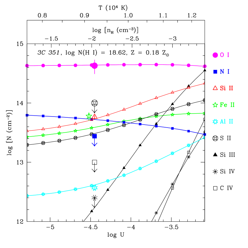
Figure 14: Model of gas photoionized by the extragalactic UV background at $z\sim$ 0 with log $N$(H I) = 18.62, Z = 0.18Z_⊙, and relative abundances following the solar pattern from Holweger (2002). Model column densities are plotted with small symbols, shown in the key at the right, as a function of the ionization parameter $U$ (lower axis) and the particle density (middle upper axis). The mean gas temperature is shown on the uppermost axis; note that the temperature scale is not linear. Observed column densities are indicated with larger symbols with 1$\sigma$ error bars. Points with arrows are 4$\sigma$ upper limits.

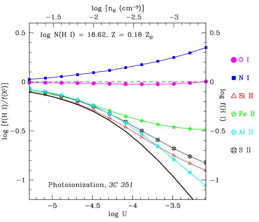
Figure 15: Ionization corrections for the photoionization model shown in Figure 14. As in Figure 13, the curves are identified at right, and the thick black line indicates $f$(H I) using the right axis.

Figure 14 shows the metal column densities predicted by the CLOUDY model as a function of $U$, and Figure 15 shows the corresponding ionization corrections from the same model over the same ionization parameter range. The best fit is obtained with log $U\approx-4.45$, as shown in Figure 14. At this value of $U$, the derived abundances are nearly identical to those derived above from the collisional ionization model. The only substantial difference between the photoionized and collisionally ionized models is for nitrogen. In the collisionally ionized model, all of the ionization correction factors of interest decrease as $T$ increases and the gas becomes more highly ionized (see Figure 13). In the photoionized model, on the other hand, the N ionization correction increases while the other ionization corrections decrease as the gas becomes more highly ionized (see Figure 15); this is due to the relatively high photoionization cross section of N I. This reduces the nitrogen underabundance implied by the measurements somewhat compared to the collisional model. However, the best-fitting photoionized model still suggests an N underabundance: we find [N/H]${}_{\rm C}\leq-1.01$ vs. [O/H]${}_{\rm C}=-0.75^{+0.17}_{-0.29}.$ If we take the lower $N$(O I) from direct integration (see Table 2 and §4), then the best fit is obtained with a somewhat higher ionization parameter, log $U\approx-3.95$ (log $n_{\rm H}\approx-2.55$). As in the collisionally ionized model, this requires a lower [O/H] by $\sim 0.2$ dex, and the nitrogen deficiency is reduced. The iron problem is also present in the photoionized calculation: if we make $\alpha-$elements overabundant in the model, then we find that the observed $N$(Fe II) is substantially greater than the predicted column density. This would be unexpected in low-metallicity gas, especially if nitrogen is underabundant.

The similarity of the photoionization and collisional ionization results is not necessarily surprising. CLOUDY includes collisional processes. The gas temperature in the photoionization model is governed by the balance of photoheating and various sources of cooling, and with the right combination of temperature and density, the collisional processes may dominate. The different behavior of N in the photoionized vs. collisionally ionized models is also not surprising. Nitrogen has a relatively large photoionization cross section, and the nitrogen + hydrogen charge exchange reaction is much weaker than that of oxygen. Consequently, N I is more readily photoionized than most species, and N I is a sensitive indicator of partially ionized gas (Sofia & Jenkins 1998). We experimented with other radiation fields in the photoionization model with various amounts of stellar flux added to the QSO background, and we found that the low-ion results did not change dramatically.

5.3 High-Velocity Ridge

The low-ion column density ratios in Complex C proper and the high-velocity ridge are strikingly alike (see Figures 8-11 and Table 2). This suggests that the physical conditions and abundances in Complex C and the HVR are quite similar. As discussed in §2, the H I column in the high-velocity ridge is not securely measured, but if we take the Green Bank measurement in Table 1 as an upper limit on the HVR $N$(H I), we obtain [O/H]_HVR $\gtrsim-1.24$ (the ionization correction should have little effect on this [O/H] estimate, as shown in Figures 13 and 15). This is consistent with the absolute metallicity derived for Complex C. However, the HV ridge contains substantially more highly ionized gas relative to the lower ionization stages. At the gas temperature and/or ionization parameter implied by the low-ion ratios in the HVR, Si IV and C IV have very small ion fractions and should be undetectable (see Table 5 in Sutherland & Dopita 1993 and Figure 14). Consequently, we conclude that the significant high ion absorption lines observed in the high-velocity ridge originate in a separate phase from the low ionization stages. The similar component structure of the low and high ions in the HVR (see Figure 7 and Figure 8e-f) suggests that there is some association between the low-ionization and high-ionization phases; this could occur if the high ions arise in an interface between the low ion-bearing gas and a hotter ambient medium.

5.4 IVC Complex C/K

The absorption-line measurements for the IVC C/K are substantially more uncertain than the HVC measurements due to line saturation and blending with adjacent components. Nevertheless, the 3C 351 spectrum indicates that C/K has a higher metallicity than Complex C proper and the HV ridge. The equivalent widths and column densities are significantly higher in the C/K component than in the high-velocity components (compare Tables 2 and 3) despite the fact that the H I column is lower in C/K than in Complex C. Adopting the O I column from profile fitting (which provides better compensation for blending and saturation) and taking $N$(H I) $<4\times 10^{18}$ cm^-2 (see § 2), we find that [O/H]${}_{\rm C/K}>-0.5$. As we have shown in the previous sections, ionization corrections are likely to be important for the other species detected in C/K. We have modeled the ionization of the C/K gas using CLOUDY, and we find that the large deficit of N I with respect to Si II shown in Figure 11 is predominantly due to ionization. At the ionization parameter that provides the best fit to the nominal O I/Si II ratio (i.e., log $U=-3.6$), the implied nitrogen underabundance is small and marginally significant, [N/O] $=-0.2^{+0.2}_{-0.3}$. The ionization-corrected abundances of the other detected species at this value of $U$ are listed in the last column of Table 3. All abundance estimates in Table 3 are listed as lower limits since we only have an upper limit on $N$(H I) (§ 2).

6 Discussion

The measurements and modeling presented in the previous sections have some interesting implications. We begin our discussion with some comments on the structure and confinement of Complex C (§6.1). We then compare the 3C 351 sight line to other nearby sight lines through this HVC (§6.2). We examine the case for metallicity variations in Complex C (§6.2.1), and then present evidence that the lower latitude region of Complex C is interacting more vigorously with the ambient medium (§6.2.2). Finally, we investigate the relationship between intermediate- and high-velocity gas observed toward H1821+643 and the HVCs in the 3C 351 spectrum (§6.2.3).

6.1 The Structure and Confinement of Complex C

Our ionization models provide constraints on the physical conditions and dimensions of the absorber. The size of the absorber along the line-of-sight is $L=N_{\rm H}/n_{\rm H}$. For the high (low) values of $N$(O I) in Complex C from Table 2, the CLOUDY models that provide the best fits to the Complex C column densities (see § 5) have $n_{\rm H}=9\times 10^{-3}\ (3\times 10^{-3})$ cm^-3, and $L=0.30\ (2.0)$ kpc, and $T\approx 9300\ (10,700)$ K. These densities and temperatures suggest that the cloud may not be gravitationally confined. Using eqn. 3 from Schaye (2001), we see that a self-gravitating cloud with these $n_{\rm H}$ and $T$ values would have a much larger size, $L=5.3\ (10)$ kpc. The self-gravitating cloud size may change by a small amount depending on the absorber geometry, as noted by Schaye. However, even with this small scale factor, the uncertainties in the parameters derived from the CLOUDY calculations do not appear to be sufficient to reconcile the large difference between the expected size for a self-gravitating cloud and the size implied by the ionization models.

The HVC could still be self-gravitating if it is predominantly composed of dark matter. Following Schaye (2001), we have assumed that the fraction of the mass in gas $f_{g}\approx\Omega_{b}/\Omega_{m}=0.16$ to calculate the self-gravitating cloud size above. The cloud could be made self-gravitating by reducing $f_{g}$ to the order of $10^{-2}-10^{-4}$. This may be unlikely, but it is not inconceivable. As an HVC plunges into a galaxy halo, ram pressure can separate the gas from its original dark matter halo (e.g., Quilis & Moore 2001). We may be viewing the small amount of residual gas in a dark matter halo that has already had most of its baryons stripped away. However, Quilis & Moore find that this requires the ambient medium to have a relatively high density, $\gtrsim 10^{-4}$ cm^-3, which they deem “unrealistic for a Galactic halo component”. However, their analysis mainly considers HVCs at distances of $\gtrsim$ 100 kpc. If Complex C is only $\sim$10 kpc away, the ambient halo density could be much higher, making this hypothesis more plausible. We note that the requirement of a small value for $f_{g}$ to make the cloud self-gravitating does not strictly require dark matter. However, searches for other components in HVCs such as stars (e.g., Willman et al. 2002) or molecular hydrogen (e.g., Richter et al. 2002) have not produced detections despite good sensitivity.

On the other hand, we may be observing the other side of this process, i.e., our gas may have been recently stripped out of a dark matter halo and is now largely devoid of dark matter. In this case, there is no particular need to confine the gas; the stripped gas could then be an ephemeral cloud that will rapidly evaporate in the hot halo.

The purely collisionally ionized model (§5.2.1) does not provide a direct constraint on the number density and hence the size of the absorber, but we argue that the situation is similar. The collisional model does provide an estimate of the H I ion fraction $f_{\rm H~{}I}$. Substituting

$$n_{\rm H}=\frac{N({\rm H~{}I})}{f_{\rm H~{}I}L}$$ (9)

into Shaye’s eqn. 3, we obtain

$$L=8.1f_{\rm H~{}I}\left(\frac{T}{10^{4}\ {\rm K}}\right)\left(\frac{N({\rm H~{}I})}{1\times 10^{20}\ {\rm cm}^{-2}}\right)^{-1}\left(\frac{f_{g}}{0.16}\right)\ {\rm kpc}.$$ (10)

The best-fit from the collisional ionization model with the high $N$(O I) has $f_{\rm H~{}I}$ = 0.43 and $T=10^{4.2}$ K, so with $N$(H I) = $4.2\times 10^{18}$ we derive $L=130$ kpc and $n_{\rm H}=2.5\times 10^{-5}$ cm^-3 from equations 9 and 10 for a gravitationally confined cloud. The angular extent of Complex C (roughly $20^{\circ}\times 90^{\circ}$) implies that the transverse size of the entire complex is $\sim 3.5\times 20$ kpc if the cloud is 10 kpc away. Therefore $L=130$ kpc requires an unlikely geometry: the cloud must be vastly larger along the line-of-sight than in the transverse direction. We reach the same conclusion with the parameters resulting from the lower O I column. This discrepancy could be reconciled, once again, by invoking a relatively small fraction of the mass in gas, $f_{g}$. The implied geometry would also be more plausible if Complex C was considerably farther than 10 kpc, but there are arguments against placing this HVC much farther away (Wakker et al. 1999a; Blitz et al. 1999). We conclude that the collisional ionization equilibrium model faces the same problems as the CLOUDY model.

Of course, there are alternatives to gravitational confinement, and there is no requirement for HVCs to contain dark matter at all. Magnetic confinement may be important (Konz, Brüns, & Birk 2002). Pressure confinement by a hotter external medium is also a reasonable alternative. The widespread detection of high-velocity O VI absorption (Sembach et al. 2002) suggests that the Milky Way has a large, hot corona. Such a corona could provide the pressure confinement that we require. The densities and temperatures from the best CLOUDY models imply that the gas pressure in the Complex C component is $p/k\approx 60-170$ cm^-3 K. If the external confining medium has $T_{\rm ext}\gtrsim 10^{6}$ K, then its density $n_{\rm ext}\lesssim 6\times 10^{-5}-2\times 10^{-4}$ cm^-3 in order to pressure confine the HVC. This density upper limit is in agreement with density constraints from other arguments (e.g., Wang 1992; Moore & Davis 1994; Weiner & Williams 1996; Murali 2000; Brüns, Kerp, & Pagels 2001). We note that these pressures are also consistent with constraints derived by Sternberg, McKee, & Wolfire (2002) on the pressure in the intragroup medium in the Local Group (based on H I structure properties in nearby dwarf galaxies).

We can apply the same analysis to the high-velocity ridge component, but we only obtain limits since we only have an upper limit on $N$(H I). For this high-velocity component, the best-fitting CLOUDY model implies an absorber thickness $L\leq$ 2.6 kpc (decreasing $N$(H I) also decreases $L$). With $n_{\rm H}\approx$ 2.5$\times 10^{-3}$ cm^-3 and $T\approx 11,300$ K, the estimated size for a self-gravitating cloud (assuming $f_{g}$ = 0.16 again) is $L=$ 11 kpc. In this case, decreasing $f_{g}$ by a factor of $2-3$ reconciles the self-gravitating cloud size with the size implied by the ionization model. Gravitational confinement appears to be viable for the HVR, as long as the actual $N$(H I) is not too much lower than our upper limit (see § 2).

Summarizing this section, our constraints on the physical conditions and dimensions of the Complex C gas toward 3C 351 indicate that it is unlikely that this absorption arises in a gravitationally confined cloud. It is much more probable that the gas is pressure confined by an external medium or is an ephemeral entity that will soon dissapate. The HVR could be gravitationally confined, but if the HVR and Complex C proper are indeed closely related, then the physical processes affecting Complex C are likely to affect the HVR as well, and the situation with the HVR may be similar to that of Complex C proper.

6.2 Sight-Line Comparisons

6.2.1 Mrk 279, Mrk 817, and PG1259+593

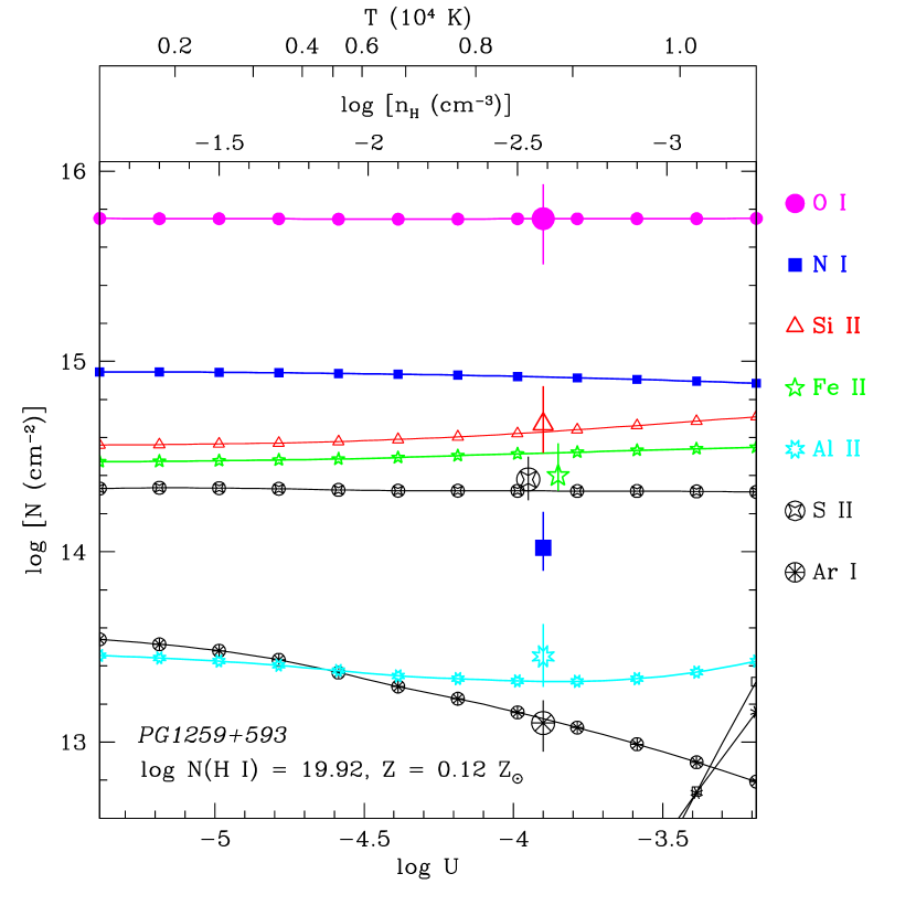
Figure 16: Model of gas photoionized by the extragalactic UV background, as in Figure 14, but with parameters appropriate for the sight line to PG1259+593: log $N$(H I) = 19.92, Z = 0.12Z_⊙, and solar relative abundances. The large points show the observed Complex C column densities in the direction of PG1259+593 from Collins et al. (2003). At log $U=-3.9$, all of the observed columns are within 1$\sigma$ of the model column densities except N I.

We can gain additional insights by comparing the 3C 351 results to other sight lines through the Complex C high-velocity cloud. Richter et al. (2001) and Collins et al. (2002) have published accurate column densities, including a variety of species, for several extragalactic sight lines through Complex C. These papers have emphasized abundance results, but the observations have implications regarding the physical conditions/structure of the HVC as well. From these papers, the spectra of Mrk 279, Mrk 817, and PG1259+593 have the highest S/N and provide the best constraints, so we shall concentrate on these sight lines.

An important difference between 3C 351 and Mrk279/Mrk817/PG1259+593 is that the latter sight lines have substantially higher H I column densities. The increased self-shielding resulting from the higher $N$(H I) has advantages and disadvantages: on the one hand, the ionization corrections are smaller, but the ion ratios also provide less leverage on the density and physical conditions of the gas. Figure 16 shows an example. This figure shows a CLOUDY calculation, analogous to the model presented in §5.2.2, of metal columns vs. log $U$ and log $n_{\rm H}$ for the sight line to PG1259+593. The only difference from the 3C 351 model is that the H I column is higher (in accord with 21cm observations), and the overall metallicity has been reduced by a small amount to provide the best fit to the observed column densities. Because of the higher $N$(H I) and greater self-shielding, most of the curves in Figure 16 are relatively flat; $f$(Xⁱ) = 1 over a large range of $U$ for most species shown. Consequently, the derived abundances are insensitive to $U$, but also most of the measurements allow a large range of $n_{\rm H}$, $L$, and $T$. However, Ar I is a notable exception. As discussed by Sofia & Jenkins (1998), Ar I is susceptible to photoionization, and this can be useful for investigation of gas ionization. This can be seen in Figure 16. While most of the curves change by 0.1 dex or less, $N$(Ar I) decreases by $\sim 0.8$ dex over the range of $U$ shown in the figure. Unfortunately, the argon lines are relatively weak, and of the eight sight lines presented by Collins et al. (2002), Ar I is only detected toward PG1259+593.

Taking advantage of the small ionization corrections, we confirm the main abundance results reported by Collins et al. (2002), with some additional important comments:

1. The Complex C oxygen abundances that we derive for these three directions show some dispersion:

   $$[{\rm O/H}]_{\rm Mrk279}=-0.59^{+0.36}_{-0.26},$$ (11)

   $$[{\rm O/H}]_{\rm Mrk817}=-0.50^{+0.25}_{-0.18},$$ (12)

   and

   $$[{\rm O/H}]_{\rm PG1259+593}=-0.91^{+0.20}_{-0.25}.$$ (13)

   However, including the 3C 351 oxygen abundance, we find that the weighted mean metallicity for Complex C is $<$[O/H]$>$ = $-0.68$ with a reduced $\chi^{2}_{\nu}=0.85$ ($\nu=3$). Therefore the current measurements are consistent with a constant metallicity throughout Complex C with $Z\approx 0.2Z_{\odot}$. Furthermore, the error bars in 11 - 13 do not fully reflect the $N$(H I) uncertainties. For example, the H I 21 cm profile toward Mrk279 is very complex, and it is difficult to separate the Complex C H I emission from the lower-velocity emission. Also, the Mrk817 $N$(H I) was derived from the larger-beam LDS data, which introduces a systematic error of $0.3-0.5$ dex. With these additional uncertainties, we conclude that there is currently no compelling evidence of oxygen abundance variations in Complex C. We cannot rule out the possibility that the oxygen abundances are spatially variable in Complex C, but better measurements are required to support this claim.

2. Nitrogen is underabundant in Complex C:

   $$[{\rm N/H}]_{\rm Mrk279}<-1.1,$$ (14)

   $$[{\rm N/H}]_{\rm Mrk817}<-1.2,$$ (15)

   $$[{\rm N/H}]_{\rm Mrk876}=-1.20^{+0.17}_{-0.15},$$ (16)

   and

   $$[{\rm N/H}]_{\rm PG1259+593}=-1.83^{+0.22}_{-0.16},$$ (17)

   where the upper limits are at the $4\sigma$ level. Again, this indicates that intermediate-mass stars have not contributed significantly to the gas enrichment. The nitrogen detections toward Mrk876 and PG1259+593 provide stronger evidence of abundance variations in Complex C than the oxygen measurements: these two sight lines yield a weighted mean of $<$[N/H]$>$ = $-1.40$ with a reduced $\chi^{2}_{\nu}$ = 5.60. Some caution is warranted, though, because $N$(N I) toward Mrk876 is entirely based on a weak and blended line (see Figure 8 in Collins et al. 2002), and the measurement may be more uncertain than the formal error bars suggest.

3. The current error bars are too large to provide significant evidence of $\alpha-$element overabundances. The model shown in Figure 16 provides a satisfactory match of the observed column densities with solar relative abundances, for example. The fact that the S II and Fe II column densities are comparable suggests that the $\alpha-$elements may be overabundant, but within current uncertainties, both [$\alpha$/Fe] = 0 and [$\alpha$/Fe] = +0.3 provide acceptable fits to the observations.

4. However, the $N$(Fe II)/$N$(S II) ratios do indicate that there is little depletion by dust in Complex C since dust strongly reduces the gas-abundance of Fe but has little effect on S in a variety of environments (e.g., Jenkins 1987; Sembach & Savage 1996).

As noted above, most metals detected along these higher $N$(H I) sight lines allow a wide range of densities and sizes. However, Ar I is useful. Toward PG1259+593, the best fit to the metals in Figure 16, including Ar I but excluding N I, has $n_{\rm H}=2.5\times 10^{-3}$, $T=8800$ K, and $L=N_{\rm H}/n_{\rm H}=13.9$ kpc. This implied size is vastly larger than the size derived from the 3C 351 data. Furthermore, in the direction of PG1259+593, gravitational confinement appears to be quite viable: this only requires $f_{g}=0.32$, i.e., a factor of two larger than Schaye’s fiducial value of 0.16. The upper limits on Complex C $N$(Ar I) for the Mrk 279 and Mrk 817 sight lines do provide the following constraints. For Mrk 279, $n_{\rm H}\lesssim 5\times 10^{-3}$ cm^-3 and $L\gtrsim$ 2.5 kpc. For Mrk 817, $n_{\rm H}\lesssim 1\times 10^{-3}$ cm^-3 and $L\gtrsim$ 14 kpc.

6.2.2 3C 351: at the Leading Edge of Complex C

Figure 17: Map of the O VI column density in Complex C proper. The xy-plane shows the $N$(H I = $2\times 10^{18}$ cm^-2 contour for Complex C from Hulsbosch & Wakker (1988), plotted vs. Galactic longitude and latitude. The z-axis shows $N$(O VI), in units of $10^{13}$ cm^-2, measured towards nine QSOs/AGNs, from Table 8 in Sembach et al. (2002). The column densities are shown with filled circles, with a line marking the sight line location within Complex C in the contour plot in the xy-plane. $N$(O VI is also projected onto the xz-plane. The location of the 3C 351 sight line is marked with a +; O VI cannot be measured in the 3C 351 spectrum because of an extragalactic Lyman limit absorber at $z_{\rm abs}=0.221$.

Figure 18: Map of the O VI/H I ratio in Complex C proper, as in Figure 17. The z-axis shows the logarithm of $N$(O VI)/$N$(H I) $\times 10^{5}$. The O VI/H I ratios are also projected onto the xz-plane, and the location of the 3C 351 sight line is marked with a +.

Why do the sight lines to 3C 351 and PG1259+593 have such starkly different implications regarding the size and confinement of the absorber? We propose a simple answer: Complex C is probably interacting with the thick disk/lower halo of the Milky Way much more vigorously in the direction of 3C 351 than in the direction of PG1259+593. This would occur naturally if the 3C 351 pencil beam is near the leading edge of the HVC, and this would explain several observations. First, the 21cm observations show a steep gradient in $N$(H I) in the vicinity of 3C 351 (see Figures 1-3). This likely reflects the transition from the mostly neutral inner region to the fully ionized periphery of the HVC. Such a transition is expected at the leading edge of a cloud moving through an ambient halo (e.g., Quilis & Moore 2001). Second, ram pressure could separate the baryons from the underlying dark matter (Quilis & Moore 2001) and thereby alleviate the confinement problem discussed above. In this case there is no compelling requirement to confine the gas; this edge of the cloud would be rapidly evaporating as it plunges toward the disk. Third, observations of nine sight lines through Complex C reported by Sembach et al. (2002) show that the O VI column densities at the velocities of Complex C are highest near 3C 351 (several of these nearby sight lines are marked in Figures 1-4). These O VI observations are summarized in Figure 17, which shows $N$(O VI) measured toward the nine extragalactic sources marked on a map of Complex C. Note that these are O VI columns in Complex C proper only; recall also that O VI cannot be measured in the 3C 351 spectrum due to a Lyman limit absorber at $z_{\rm abs}=0.221$ that severely attenuates the FUSE 3C 351 spectrum below $\sim$1117 Å. As shown in Figure 18, an even more pronounced trend is evident in the $N$(O VI)/$N$(H I) ratio in Complex C. This ratio increases steadily with decreasing longitude and latitude, and the lowest-longitude Complex C sight line (Mrk 501; see Table 8 in Sembach et al. 2002) has an $N$(O VI)/$N$(H I) ratio which is $\sim$43 times larger than the ratio measured toward the highest-longitude sight line (PG1259+593). This trend also suggests that the lower-longitude section of Complex C is more strongly interacting with the ambient medium; as the gas is ionized to a greater degree, $N$(H I) will decrease while $N$(O VI) increases. The lower-longitude region is also at lower latitude, so this result is not surprising: as the HVC approaches the plane of the Milky Way, it is becoming more fully ionized and is probably ablating and dissipating, and the trailing (higher-longitude) portion of the cloud has not yet entered the higher density region of the ambient medium where the interactions are more vigorous, or at least has not suffered the effects of ablation for the same duration as the lower latitude/longitude regions.

6.2.3 H1821+643

An alternative to the interpretation presented above is that gas flowing up out of the disk (e.g., Galactic fountain/chimney gas) is colliding with Complex C at lower longitudes and latitudes, and the resultant shock-heating is ionizing and evaporating the cloud. Gibson et al. (2001) and Collins et al. (2002) have suggested that such interactions might be required to explain the metallicity variations observed in the HVC (but see point 1 in §6.2.1). In this regard, it is interesting to compare the 3C 351 to the H1821+643 sight line, which is near 3C 351 but closer to the plane (see Figures 1-4). The H1821+643 line-of-sight passes just outside the lower-latitude 21cm boundary of Complex C (see also Figure 1 in Wakker & van Woerden 1997) but through the region of high-velocity emission associated with the Outer Arm. A good spectrum of H1821+643 could reveal gas flowing from the plane toward Complex C.

Savage, Sembach, & Lu (1995) have discussed Galactic absorption features in the spectrum of H1821+643 based on an intermediate-resolution GHRS spectrum. Subsequently, Tripp, Savage, & Jenkins (2000) obtained a higher resolution STIS spectrum of H1821+643 with the same mode (E140M) used to observe 3C 351, so a detailed comparison of these sight lines can be made without confusion due to differing spectral resolution. Figure 19 compares selected absorption profiles observed toward H1821+643 (upper profile in each panel) to the same line from the spectrum of 3C 351. For reference, the velocities of the HVR, C, and C/K components are marked at the top of each panel. Some of the profiles appear to be remarkably similar, e.g., the Fe II lines in Figure 19d. We defer a full analysis of the H1821+643 data to a later paper, but a few comments on this figure are worthwhile.

Figure 19: Comparison of normalized absorption profiles observed in the directions of 3C 351 (lower profile in each panel) and H1821+643 (upper profile in each panel). The plots compare the (a) O I $\lambda$1302.17, (b) Si II $\lambda$1304.37, (c) Al II $\lambda$1670.79, (d) Fe II $\lambda$1608.45, (e) Si III $\lambda$1206.50, and (f) C IV $\lambda$1548.20 transitions. The H1821+643 spectra have been offset by +1 for clarity. These sight lines probe the low-latitude edge of Complex C (see Figures 1 - 3 as well as Figure 1 in Wakker & van Woerden 1997). For reference, the velocities of the high-velocity ridge (HVR), Complex C, and IVC C/K are marked at the top of each panel.

The v = $-$80 km s^-1 component: Complex C/K. Both sight lines show components near the velocity of IVC C/K with similar equivalent widths. Toward H1821+643, Savage et al. (1995) associate this absorption with the Perseus spiral arm, which has a similar velocity at $b\approx 0$ and appears to extend $\sim 1$ kpc above the plane based on 21cm and H$\alpha$ emission (Kepner 1970; Reynolds 1986). We have derived [O/H] $>-0.5$ for the C/K component toward 3C 351, implying a higher metallicity than the adjacent Complex C and HVR components. The higher C/K metallicity suggests that this gas may indeed have originated in the disk and is being driven into the halo. If the Perseus arm is $\sim 3$ kpc away and the 3C 351 C/K component is associated with Perseus, then this gas is $\sim 2$ kpc above the plane. This is consistent with the $z-$heights that gas is expected to attain in some Galactic fountain models (e.g., Houck & Bregman 1990). Very recently, Otte, Dixon, & Sankrit (2003) have detected O VI emission at $v_{\rm LSR}=-50\pm 30$ km s^-1 from $l=95.4^{\circ}$, $b=36.1^{\circ}$, a direction very close to the 3C 351 and H1821+643 sight lines. They also show bright H$\alpha$ filaments extending up from the plane in this direction. They attribute both the O VI and H$\alpha$ emission to an outflow from the Perseus arm. Regardless of the nature of the gas, it is quite likely that the absorption lines at $v\approx-80$ km s^-1 toward 3C 351 and H1821+643 are related to the emission reported by Otte et al. (2003).

The v = $-$130 km s^-1 component: Complex C vs. the Outer Arm. Strong absorption lines are present at the velocity of Complex C in the spectra of both H1821+643 and 3C 351. However, unlike IVC C/K, the line equivalent widths in the H1821+643 spectrum are substantially larger than the same lines toward 3C 351 at $v=-130$ km s^-1 (see Figure 19). The H1821+643 and 3C 351 21 cm H I column densities at this velocity are similar: Wakker et al. (2001) report $N$(H I) = $3.3\times 10^{18}$ toward H1821+643, compared to $N$(H I) = $4.2\times 10^{18}$ toward 3C 351 (both measurements are based on Effelsberg observations). However, there is a gap in the 21 cm emission between the two sight lines (see Figures 1 and 3), and the relationship (if any) between the 3C 351 and H1821+643 HVCs at this velocity is unclear. We list in Table 4 the equivalent widths and column densities of absorption lines at $v=-130$ km s^-1 in the H1821+643 spectrum, measured as described in § 4. Several pixels in the core of the O I line toward H1821+643 approach zero flux. This line may be significantly saturated, so we consider the O I measurements highly uncertain. The most conservative constraint on $N$(O I) is a lower limit from direct integration, but we also provide an estimate from profile fitting in Table 4, which can correct somewhat for saturation but with large uncertainties. We also summarize the implied abundances in Table 4 as before, without and with ionization corrections applied (using the ionization model presented below).

Table 4: High-Velocity Absorption Lines toward H1821+643: The Outer Arm

Species	$\lambda_{0}$	$<v>$	$W_{\lambda}$	log $N_{\rm a}$	log $N_{\rm pf}$	[Xi/H I]	[X/H]
	(Å)	(km s-1)	(mÅ)
O I	1302.17	$-131\pm 1$	183.6$\pm$5.4	$>14.70$	15.18${}^{+0.26}_{-0.24}$	$\geq-0.55$	$\geq-0.57$
N I	1199.55	$-136\pm 5$	40.0$\pm$9.3	13.47$\pm 0.11$	$13.40\pm 0.09$	$-0.97\pm 0.17$	$-0.73\pm 0.17$
Si II	1304.37	$-128\pm 1$	134.0$\pm$4.4	$14.18\pm 0.02$	14.18${}^{+0.11}_{-0.09}$	$0.13^{+0.14}_{-0.12}$	$-0.66^{+0.14}_{-0.12}$
	1526.71	$-129\pm 1$	196.6$\pm$6.0	$14.15\pm 0.04$	14.18${}^{+0.11}_{-0.09}$	$0.13^{+0.14}_{-0.12}$	$-0.66^{+0.14}_{-0.12}$
Al II	1670.79	$-128\pm 1$	222.8$\pm$10.0	12.98$\pm$0.04	$13.02\pm 0.04$	$0.00\pm 0.11$	$-0.80\pm 0.11$
Fe II	1608.45	$-131\pm 1$	79.3$\pm$5.4	13.88$\pm$0.04	13.89$\pm 0.04$	$-0.08\pm 0.12$	$-0.60\pm 0.12$

Table 5: High-Velocity Absorption Lines toward H1821+643: The -212 km s^-1 Component

Species	$\lambda_{0}$	$<v>$	$W_{\lambda}$	log $N_{\rm a}$	log $N_{\rm pf}$
	(Å)	(km s-1)	(mÅ)
O I	1302.17	$\cdots$	$3.8\pm 4.7$	$<13.38$	$\cdots$
C II	1334.53	$\cdots$	$7.6\pm 3.4$	$<12.84$	$\cdots$
Si III	1206.50	$\cdots$	$-3.9\pm 8.6$	$<12.21$	$\cdots$
Si IV	1393.76	$\cdots$	$10.0\pm 4.6$	$<12.32$	$\cdots$
C IV	1548.20	$-212\pm 1$	$52.4\pm 5.5$	$13.22\pm 0.05$	$13.24\pm 0.03$
N V	1238.82	$\cdots$	$7.4\pm 5.4$	$<13.01$	$\cdots$
O VI	1031.93	$-192$	$\cdots$	13.72$\pm$0.14	$\cdots$

The larger equivalent widths toward H1821+643 at $v_{\rm LSR}\approx-130$ km s^-1 ostensibly indicate that the metallicity at this velocity is greater in the H1821+643 component than in the 3C 351 HVC since the H I columns are similar toward both QSOs. If we neglect ionization corrections, we indeed obtain high abundances from the column densities in Table 4, e.g., [O I/H I] $\gtrsim-0.6$, [Si II/H I] = 0.13, [Al II/H I] = 0.0, and [Fe II/H I] = $-0.08$, but with a surprisingly low nitrogen abundance, [N I/H I] = $-0.97$. This would be an unusual abundance pattern; N underabundances are expected in low-metallicity gas, but as $Z\longrightarrow Z_{\odot}$, the contribution from intermediate-mass stars is expected to bring the N relative abundance more in line with the solar value. However, we have shown in § 5 that ionization corrections must not be neglected when $N$(H I) is at the level observed toward H1821+643. When ionization corrections are applied, the observed columns can be reconciled with a lower overall metallicity and smaller N underabundances. Figure 20 shows a CLOUDY model in satisfactory agreement with the observed columns with $Z=0.24Z_{\odot}$ and only small underabundance of N and Al. The model shown in Figure 20 works if $N$(O I) is close to the value from direct integration, i.e., $N$(O I) $\approx$ 14.7. Higher O I column densities would require higher metallicity, lower ionization parameters (to match, e.g., the O I/Si II ratio), and greater nitrogen underabundances, as can be seen from Figure 20. A slight depletion of Fe might also be required in higher metallicity models. Due to the large range of $U$ allowed by the current data, we cannot usefully bracket the size of the absorber at $v_{\rm LSR}=-130$ km s^-1.

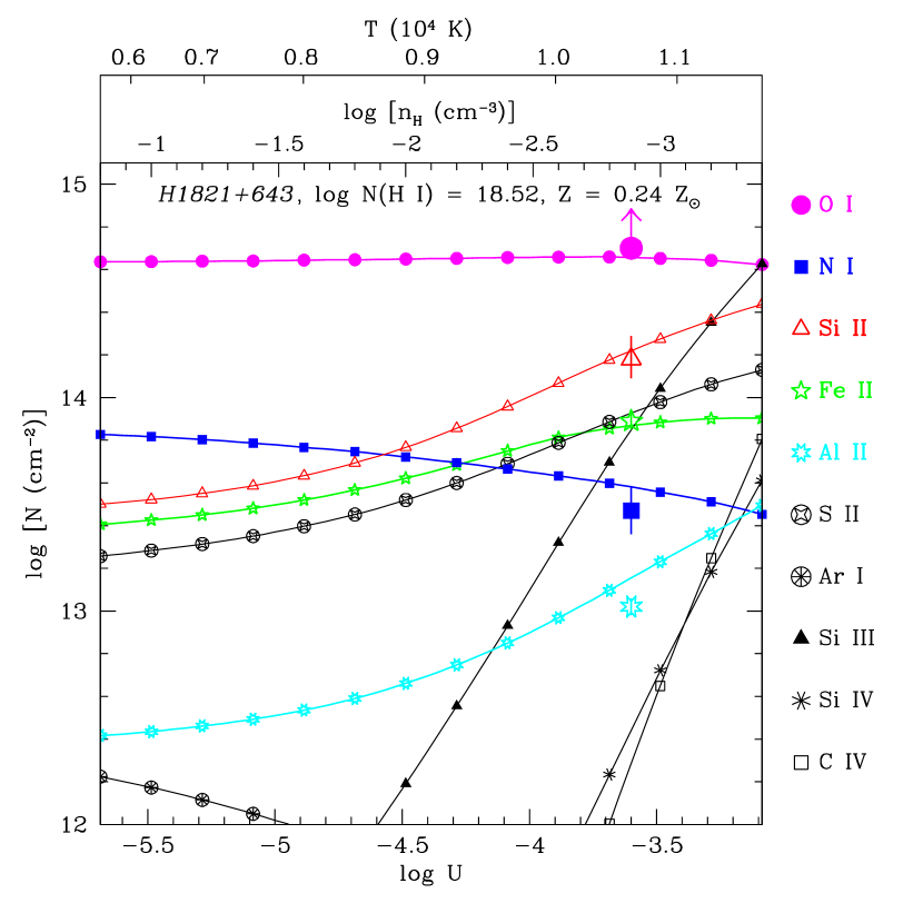
Figure 20: Model of gas photoionized by the extragalactic UV background, as in Figure 14, but with parameters appropriate for the Outer Arm component in the spectrum of H1821+643. The large points show the observed Outer Arm column densities toward H1821+643. At log $U=-3.6$, the model is in reasonable agreement with the observed column densities. However, $N$(O I) may be underestimated due to saturation; to fit the observations with a higher O I column density, $U$ must decrease and the metallicity must increase.

At this juncture, it remains possible that the Outer Arm high-velocity gas and Complex C have similar metallicities, but the data also allow the Outer Arm to have a substantially higher metallicity than Complex C if N is underabundant. Consequently, it is difficult to draw firm conclusions about the relationship between the Outer Arm and Complex C. Weaker O I lines in the FUSE bandpass may help to more tightly constrain the metallicity of the Outer Arm and thereby clarify this relationship.

The v = $-$200 km s^-1 component: the high-velocity ridge. Finally, it is interesting to compare the 3C 351 and H1821+643 sight lines at the velocity of the HVR component, $v_{\rm LSR}\approx-200$ km s^-1. While the HVR absorption is clearly detected in a variety of transitions toward 3C 351, most of the H1821+643 profiles show nothing at this velocity (the Si III profiles in panel (e) of Figure 19 show the contrast between the sight lines at this $v$). However, Savage et al. (1995) tentatively identified C IV absorption near this velocity in a GHRS spectrum of H1821+643. As shown in Figure 21, we confirm this detection: both lines of the C IV $\lambda\lambda$1548.2, 1550.8 doublet are well-detected at $v=-212$ km s^-1. These are the only lines that we detect in the STIS spectrum at this velocity. The C IV equivalent width and column density measurements are listed in Table 5 along with upper limits on selected dominant ions and higher stages. However, Oegerle et al. (2000) and Sembach et al. (2000) detected O VI at this velocity in FUSE spectra of H1821+643. The O VI 1031.9 Å line is blended with low-velocity H₂, but Sembach et al. (2002) have removed the H₂ line (based on fits to other H₂ lines) and find log $N$(O VI) = $13.72\pm 0.14$.

These measurements have useful implications. The fact that $N$(O VI) $\gg$ $N$(C IV) toward H1821+643 would indicate that $T\gg 10^{5}$ K if the gas were collisionally ionized and in equilibrium (see, e.g., Figure 7 in Tripp & Savage 2000). However, this temperature is not compatible with the widths of the C IV lines. Figure 21 shows our Voigt-profile fit to the HVR features in the H1821+643 spectrum; a single component with $b=9\pm 2$ provides an excellent fit. This implies that $T<10^{4.77}$ K. The C IV line width is only marginally consistent with the O VI/C IV ratio given the uncertainties in $N$(O VI) and $b$(C IV). It seems more likely that either (1) much of the O VI absorption is not associated with the C IV-bearing gas (in which case the O VI-gas must be relatively hot to satisfy the lower limit on O VI/C IV), or (2) the gas is not in ionization equilibrium. The different centroids of the C IV and O VI lines (see Table 5) support the idea that at least some of the O VI originates in different gas. It is unlikely that the C IV + O VI gas is photoionized because of the long pathlengths required (e.g., Sembach et al. 2002), but it is possible that the gas is collisionally ionized but out of equilibrium because it is cooling faster than it can recombine (Edgar & Chevalier 1986). Heckman et al. (2002) have recently shown that a non-equilibrium, radiatively cooling gas model provides a good fit to the O VI column densities and $b-$values in HVCs (as well as other contexts). Their model also predicts $N$(O VI) $\gg$ $N$(C IV), as observed in the $-200$ km s^-1 feature toward H1821+643.

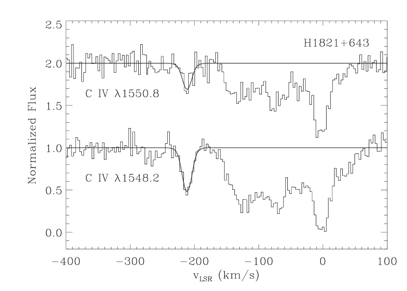
Figure 21: Continuum-normalized C IV absorption profiles observed toward H1821+643. The upper histogram shows the $\lambda$1550.8 transition and the lower histogram is the $\lambda$1548.2 line. The fit to the component at $v_{\rm LSR}=-212$ km s^-1 is overplotted with a solid line.

Savage et al. (1995) have noted that $v_{\rm LSR}\approx-200$ km s^-1 is near the expected velocity for distant Milky Way gas in a corotating disk/halo in the direction of H1821+643; the velocity would then imply a large Galactocentric distance (see their Figure 2). However, it is quite possible that this high-velocity feature is associated with the high-velocity ridge observed toward 3C 351 and other sight lines. In this case, the fact that the feature is only detected in C IV and O VI would indicate that the HVR has an extended ionized periphery. Evidence for highly-ionized layers on the surface of HVCs has been reported for other clouds (e.g., Sembach et al. 1999). We have argued that the absorption lines toward 3C 351 indicate that the HVR and Complex C proper are related. If the $v_{\rm LSR}=-212$ km s^-1 component toward H1821+643 is also part of the HVR, then this gas is likely much closer than implied by its velocity and the assumption that it is corotating (various arguments suggest that Complex C is $\sim$10 kpc from the Sun).

7 Summary

We have investigated the physical structure, conditions, metallicity, and nature of the high-velocity cloud Complex C using high-resolution recordings of absorption lines in several directions through the cloud. Our study is mainly based on STIS echelle spectroscopy of 3C 351, which shows a wide variety of absorption lines from Complex C proper ($v_{\rm LSR}=-128$ km s^-1) as well as an intermediate-velocity cloud (C/K, $v_{\rm LSR}=-82$ km s^-1) and a higher-velocity component that we refer to as the high-velocity ridge ($v_{\rm LSR}=-190$ km s^-1). We also make use of other sight lines through Complex C from the literature as well as new STIS echelle observations of H1821+643, which is just outside the 21 cm boundary of Complex C but shows absorption lines at very similar velocities to those seen toward 3C 351. From our analysis, we reach the following conclusions:

1. The high-velocity ridge is closely related to Complex C proper. This is suggested by the similar morphologies of the HVR and Complex C; the HVR has a similar shape and is roughly centered on the larger, lower-velocity Complex C. This idea is supported by the absorption lines, which show remarkably similar column density ratios in the HVR and Complex C. However, very little high-ion absorption is detected at the velocity of Complex C proper, but Si III, Si IV, and C IV absorption is strong and easily detected in the HVR. Moreover, the high-ion absorption lines in the HVR have centroids and line widths that are similar to those of the low ions in the HVR. We show that the high and low ionization stages in the HVR cannot arise in the same phase, and we conclude that the high ion absorption occurs in an interface between the low-ionization phase and a hotter ambient medium.

2. The relative abundances in all components with $N$(H I) $<10^{19}$ cm^-2 indicate that ionization corrections are important. We consider collisional ionization equilibrium as well as CLOUDY photoionization models to derive ionization corrections, and we find in both cases that $Z=(0.2\pm 0.1)Z_{\odot}$ in Complex C in the direction of 3C 351. We also find that nitrogen must be underabundant toward 3C 351. The low metallicity and nitrogen underabundance indicate that Complex C is not ejecta generated in a Galactic fountain. It seems more likely that Complex C is either tidally stripped material from a satellite galaxy (analogous to the Magellanic Stream), or that it is gas with a more distant extragalactic origin. The absolute metallicity of the 3C 351 HVR component is less constrained because we only have an upper limit on the HVR H I column. The lower limits on the HVR metallicity are consistent with the metallicity derived for Complex C proper.

3. We find similar oxygen abundances at Complex C velocities toward Mrk 279, Mrk 817, and PG1259+593. While there is some dispersion in the [O/H] measurements, within the current uncertainties the measurements are fully consistent with a constant metallicity throughout the HVC. These sight lines as well as the Mrk 876 sight line also provide strong evidence of N underabundances in Complex C. Comparison of the nitrogen abundances toward Mrk 876 and PG1259+593 provides the strongest evidence of spatial abundance variability in Complex C, but this requires confirmation with additional measurements. There are hints of $\alpha-$element overabundances in some directions, but the evidence is not statistically significant.

4. The derived iron abundances indicate that Complex C contains little or no dust.

5. Toward 3C 351, the Complex C absorber size, density, and temperature implied by the ionization models indicate that the gas is not gravitationally confined, while toward other sight lines such as PG1259+593, the implied path length through Complex C is much larger and gravitational confinement is viable. Pressure confinement by an external medium may play a role. However, we suggest that the 3C 351 sight line passes through the leading edge of Complex C, which has been ablating and dissipating as it approaches the plane of the Milky Way. This idea is supported by O VI observations, which show the highest O VI column densities near the 3C 351 sight line. Furthermore, the O VI/H I ratio increases dramatically with decreasing longitude and latitude within Complex C, which also suggests that the lower longitude and latitude regions are interacting more vigorously with the ambient medium.

6. To look for evidence of outflowing Milky Way gas that might interact with Complex C, we compare the STIS echelle observations of the sight lines to 3C 351 and H1821+643, which are both near the lower-latitude edge of Complex C at $l\approx 90^{\circ}$. We find that the intermediate-velocity gas observed toward both of these QSOs likely has a higher metallicity and may indeed be a fountain/chimney outflow from the Perseus spiral arm. Unfortunately, the results are less clear for the high-velocity gas toward H1821+643. The H1821+643 HVC could have a similar metallicity to that derived for Complex C, or it could have a much higher abundance depending on the O I column and ionization correction, both of which are highly uncertain.

References

- (1) Afflerbach, A., Churchwell, E., & Werner, M. W. 1997, ApJ, 478, 190
- (2) Allende Prieto, C., Lambert, D. L., & Asplund, M. 2001, ApJ, 556, L63
- (3) Bland-Hawthorn, J., Beilleux, S., Cecil, G. N., Putman, M. E., Gibson, B. K., & Maloney, P. R. 1998, MNRAS, 299, 611
- (4) Bland-Hawthorn, J. & Maloney, P. 2002, in Extragalactic Gas at Low Redshift, eds. J. S. Mulchaey & J. T. Stocke, ASP Conf. Ser. 254, 267
- (5) Blitz, L., Spergel, D. N., Teuben, P. J., Hartmann, D., & Burton, W. B. 1999, ApJ, 514, 818
- (6) Bowen, D. V., Blades, J. C., & Pettini, M. 1995, ApJ, 448, 662
- (7) Bowers, C. W., et al. 1998, Proc. SPIE, 3356, 401
- (8) Braun, R. & Burton, W. B. 1999, A&A, 341, 437
- (9) Braun, R., & Burton, W. B. 2001, A&A, 375, 219
- (10) Bregman, J. N. 1980, ApJ, 236, 577
- (11) Brüns, C., Kerp, J., & Pagels, A. 2001, A&A, 370, 26
- (12) Charlton, J. C., Churchill, C. W., & Rigby, J. R. 2000, 544, 702
- (13) Collins, J. A., Shull, J. M., & Giroux, M. L. 2003, ApJ, 585, 336
- (14) Cowie, L. L., Songaila, A., & York, D. G. 1979, ApJ, 230, 469
- (15) Delhaye, J. 1965, in Galactic Structure, Stars and Stellar Systems, Vol. 5, eds. A. Blaauw & M. Schmidt, (Chicago: University of Chicago Press), 61
- (16) Edgar, R. J., & Chevalier, R. A. 1986, ApJ, 310, L27
- (17) Ferland, G. J., Korista, K. T., Verner, D. A., Ferguson, J. W., Kingdon, J. B., & Verner, E. M. 1998, PASP, 110, 761
- (18) Field, G. B., & Steigman, G. 1971, ApJ, 166, 59
- (19) Fitzpatrick, E. L., & Spitzer, L. 1997, ApJ, 475, 623
- (20) Gibson, B. K. 2002, in ASP Conf. Ser. 273, The Dynamics, Structure, and History of Galaxies, eds. G. S. Da Costa & H. Jerjen, (San Francisco: ASP), 205
- (21) Gibson, B. K., Fenner, Y., Maddison, S. T., & Kawata, D. 2002, in ASP Conf. Ser. 254, Extragalactic Gas at Low Redshift, eds. J. S. Mulchaey & J. T. Stocke, (San Francisco: ASP), 225
- (22) Gibson, B. K., Giroux, M. L., Penton, S. V., Stocke, J. T., Shull, J. M., & Tumlinson, J. 2001, AJ, 122, 3280
- (23) Grevesse, N., Noels, A., Sauval, A. J. 1996, in ASP Conf. Ser. 99, Cosmic Abundances, eds. S. S. Holt & G. Sonneborn, (San Francisco: ASP), 117
- (24) Grevesse, N., & Sauval, A. J. 1998, SSRv, 85, 161
- (25) Haardt, F., & Madau, P. 1996, ApJ, 461, 20
- (26) Haffner, L. M., Reynolds, R. J., & Tufte, S. L. 2001, ApJ, 556, L33
- (27) Heckman, T. M., Norman, C. A., Strickland, D. K., & Sembach, K. R. 2002, ApJ, 577, 691
- (28) Henry, R. B. C., Edmunds, M. G., & Köppen, J. 2000, ApJ, 541, 660
- (29) Holweger, H. 2001, in Joint SOHO/ACE Workshop, Solar and Galactic Composition, AIP Conf. Proc. 598, ed. R. F. Wimmer-Schweingruber, (New York: AIP), 23 (astro-ph/0107426)
- (30) Houck, J., & Bregman, J. N. 1990, ApJ, 352, 506
- (31) Jenkins, E. B. 1987, in Interstellar Processes, eds. D. J. Hollenbach & H. A. Thronson, (Dordrecht: Reidel), 533
- (32) Jenkins, E. B. 1996, ApJ, 471, 292
- (33) Jenkins, E. B., et al. 1998, ApJ, 492, L147
- (34) Jenkins, E. B., & Peimbert, A. 1997, ApJ, 477, 265
- (35) Jenkins, E. B., Woźniak, P. R., Sofia, U. J., Sonneborn, G., & Tripp, T. M. 2000, ApJ, 538, 275
- (36) Kepner, J., Tripp, T. M., Abel, T., & Spergel, D. 1999, AJ, 117, 2063
- (37) Kepner, M. 1970, A&A, 5, 444
- (38) Kerr, F. J., & Lynden-Bell, D. 1986, MNRAS, 221, 1023
- (39) Kimble, R. A., et al. 1998, ApJ, 492, L83
- (40) Klypin, A., Kravtsov, A. V., Valenzuela, O., & Prada, F. 1999, ApJ, 522, 82
- (41) Konz, C., Brüns, C., & Birk, G. T. 2002, A&A, 391, 713
- (42) Konz, C., Lesch, H., Birk, G. T., & Wiechen, H. 2001, ApJ, 548, 249
- (43) Larson, R. B. 1972, Nature, 236, 21
- (44) Lauroesch, J. T., Truran, J. W., Welty, D. E., & York, D. G. 1996, PASP, 108, 641
- (45) Leitherer, C., et al. 2001, STIS Instrument Handbook, Version 5.1 (Baltimore:STScI)
- (46) Lockman, F. J., Murphy, E. M., Petty-Powell, S., & Urick, V. J. 2002, ApJS, 140, 331
- (47) Mac Low, M.-M., & Ferrara, A. 1999, ApJ, 513, 142
- (48) Mathewson, D. S., Cleary, M. N., & Murray, J. D. 1974, ApJ, 190, 291
- (49) McWilliam, A. 1997, ARA&A, 35, 503
- (50) Meyer, D. M., Cardelli, J. A., & Sofia, U. J. 1997, ApJ, 490, L103
- (51) Moore, B., & Davis, M. 1994 MNRAS, 270, 209
- (52) Moore, B., Ghigna, S., Governato, F., Lake, G., Quinn, T., Stadel, J., & Tozzi, P. 1999, ApJ, 524, L19
- (53) Moos, H. W., et al. 2002, ApJS, 140, 3
- (54) Morton, D. C. 1991, ApJS, 77, 119
- (55) Morton, D. C. 2002, in preparation
- (56) Murali, C. 2000, ApJ, 529, L81
- (57) Murphy, E. M., et al. 2000, ApJ, 538, L35
- (58) Murphy, E. M., Sembach, K. R., & Lockman, F. J. 2002, private communication
- (59) Oegerle, W. R., Tripp, T. M., Sembach, K. R., Jenkins, E. B., Bowen, D. V., Cowie, L. L., Green, R. F., Kruk, J. W., Savage, B. D., Shull, J. M., & York, D. G. 2000, ApJ, 538, L23
- (60) Oort, J. H. 1970, A&A, 7, 381
- (61) Otte, B., Dixon, W. V., & Sankrit, R. 2003, ApJ, in press (astro-ph/0302251)
- (62) Penton, S. V., Shull, J. M., & Stocke, J. T. 2000, ApJ, 544, 150
- (63) Pisano, D. J., & Wilcots, E. M. 2003, ApJ, 584, 228
- (64) Putman, M. E., et al. 1998, Nature, 394, 752
- (65) Quilis, V., & Moore, B. 2001, ApJ, 555, L95
- (66) Reynolds, R. J. in Gaseous Halos of Galaxies, ed. J. N. Bregman & F. J. Lockman (Greenbank: NRAO), 53
- (67) Richter, P., Sembach, K. R., Wakker, B. P., Savage, B. D., Tripp, T. M., Murphy, E. B., Kalberla, P. M. W., & Jenkins, E. B. 2001, ApJ, 559, 318
- (68) Richter, P., Wakker, B. P., Savage, B. D., & Sembach, K. R. 2002, ApJ, in press (astro-ph/0211356)
- (69) Savage, B. D., & Sembach, K. R. 1991, ApJ, 379, 245
- (70) Savage, B. D., Sembach, K. R., & Lu, L. 1995, ApJ, 449, 145
- (71) Schaye, J. 2001, ApJ, 559, 507
- (72) Sembach, K. R., et al. 2000, ApJ, 538, L31
- (73) Sembach, K. R., et al. 2002, ApJS, astro-ph/0207562
- (74) Sembach, K. R., & Savage, B. D. 1992, ApJS, 83, 147
- (75) Sembach, K. R., & Savage, B. D. 1996, ApJ, 457, 211
- (76) Sembach, K. R., Savage, B. D., Lu, L., & Murphy, E. M. 1999, ApJ, 515, 108
- (77) Shapiro, P., & Field, G. 1976, ApJ, 205, 762
- (78) Sofia, U. J., & Jenkins, E. B. 1998, ApJ, 499, 951
- (79) Sofia, U. J., & Meyer, D. M. 2001, ApJ, 554, L221
- (80) Sternberg, A., McKee, C. F., & Wolfire, M. G. 2002, 143, 419
- (81) Sutherland, R. S., & Dopita, M. A. 1993, ApJS, 88, 253
- (82) Tosi, M. 1988, A&A, 197, 47
- (83) Trapero, J., Welty, D. E., Hobbs, L. M., Lauroesch, J. T., Morton, D. C., Spitzer, L., & York, D. G. 1996, ApJ, 468, 290
- (84) Tripp, T. M., Giroux, M. L., Stocke, J. T., Tumlinson, J., & Oegerle, W. R. 2001, ApJ, 563, 724
- (85) Tripp, T. M., & Savage, B. D. 2000, ApJ, 542, 42
- (86) Tripp, T. M., Savage, B. D., & Jenkins, E. B. 2000, ApJ, 534, L1
- (87) Tripp, T. M., et al. 2002, ApJ, 575, 697
- (88) Tufte, S. L., Reynolds, R. J., & Haffner, L. M. 1998, ApJ, 504, 773
- (89) Tufte, S. L., Wilson, J. D., Madsen, G. J., Haffner, L. M., & Reynolds, R. J. 2002, ApJ, 572, L153
- (90) van Woerden, H., Peletier, R. F., Schwarz, U. J., Wakker, B. P., & Kalberla, P. M. W. 1999, in ASP Conf. Ser. 166, Stromlo Workshop on High-Velocity Clouds, ed. B. K. Gibson & M. E. Putman, (San Francisco: ASP), 1
- (91) Vila-Costas, M. B., & Edmunds, M. G. 1993, MNRAS, 265, 199
- (92) Wang, Q. D. 1992, PASP, 104, 812
- (93) Wakker, B. P. 2001, ApJS, 136, 463
- (94) Wakker, B. P., et al. 1999a, Nature, 402, 388
- (95) Wakker, B. P., et al. 2002, ApJS, submitted, astro- ph/0208009
- (96) Wakker, B. P., Howk, J. C., Savage, B. D., Tufte, S. L., Reynolds, R. J., van Woerden, H., Schwarz, U. J., & Peletier, R. F. 1999b, in ASP Conf. Ser. 166, Stromlo Workshop on High Velocity Clouds, ed. B. K. Gibson & M. E. Putman (San Francisco: ASP), 26
- (97) Wakker, B. P., Kalberla, P. M. W., van Woerden, H., de Boer, K. S., & Putman, M. E. 2001, ApJS, 136, 537
- (98) Wakker, B. P., & van Woerden, H. 1997, ARA&A, 35, 217
- (99) Weiner, B. J., Vogel, S. N., & Williams, T. B. 2002, in Extragalactic Gas at Low Redshift, eds. J. S. Mulchaey & J. T. Stocke, ASP Conf. Ser. 254, 256
- (100) Weiner, B. J., & Williams, T. B. 1996, AJ, 111, 1156
- (101) Welty, D. E., Hobbs, L. M., Lauroesch, J. T., Morton, D. C., Spitzer, L., & York, D. G. 1999, ApJS, 124, 465
- (102) Weymann, R. J., Vogel, S. N., Veilleux, S., & H. W. Epps 2001, ApJ, 561, 559
- (103) Willman, B., Dalcanton, J., Ivezic, Z., Schneider, D. P., & York, D. G. 2002, AJ, 124, 2600
- (104) Yuan, Q., Green, R. F., Brotherton, M., Tripp, T. M., Kaiser, M. E., & Kriss, G. A. 2002, ApJ, 575, 687
- (105) Zwaan, M. A. 2001, MNRAS, 325, 1142
- (106) Zwaan, M. A., & Briggs, F. H. 2000, ApJ, 530, L61