Thermal Conduction in Magnetized Turbulent Gas

Abstract

Using numerical methods, we systematically study in the framework of ideal MHD the effect of magnetic fields on heat transfer within a turbulent gas. We measure the rates of passive scalar diffusion within magnetized fluids and make the comparisons a) between MHD and hydro simulations, b) between different MHD runs with different values of the external magnetic field (up to the energy equipartition value), c) between thermal conductivities parallel and perpendicular to magnetic field. We do not find apparent suppression of diffusion rates by the presence of magnetic fields, which implies that magnetic fields do not suppress heat diffusion by turbulent motions.

1 Astrophysical Motivation

It is well known that Astrophysical fluids are turbulent and that magnetic fields are dynamically important. One characteristic of the medium that magnetic fields and turbulence may substantially change is the heat transfer.

There are many instances when heat transfer through thermal conductivity is important. For instance, thermal conductivity is essential in rarefied gases where radiative heat transfer is suppressed. This is exactly the situation that is present in clusters of galaxies. It is widely accepted that ubiquitous X-ray emission due to hot gas in clusters of galaxies should cool significant amounts of the intracluster medium (ICM) and this must result in cooling flows (Fabian 1994). However, observations do not support the evidence for the cool gas (see Fabian et al. 2001) which is suggestive of the existence of heating that replenishes the energy lost via X-ray emission. Heat transfer from the outer hot regions can do the job, provided that the heat transfer is sufficiently efficient.

Gas in clusters of galaxies is magnetized and the conventional wisdom suggests that the magnetic fields strongly suppress thermal conduction perpendicular to their direction. Realistic magnetic fields are turbulent and the issue of the thermal conduction in such a situation has been long debated. A recent paper by Narayan & Medvedev (2001) obtained estimates for the thermal conductivity of turbulent magnetic fields, but those estimates happen to be too low to explain the absence of cooling flows for many of the clusters of galaxies (Zakamska & Narayan 2002).

Narayan & Medvedev (2001) treat the turbulent magnetic fields as static. In hydrodynamical turbulence it is possible to neglect plasma turbulent motions only when the diffusion of electrons which is the product of the electron thermal velocity $v_{elect}$ and the electron mean free path in plasma $l_{mfp}$, i.e. $v_{elect}l_{mfp}$, is greater than the turbulent velocity $v_{turb}$ times the turbulent injection scale $l_{inj}$, i.e. $v_{turb}l_{inj}$. If such scaling estimates are applicable to heat transport in magnetized plasma, the turbulent heat transport should be accounted for heat transfer within clusters of galaxies. Indeed, data for $v_{elect}l_{mfp}$ given in Zakamska & Narayan (2002; Narayan & Medvedev 2001) provide the classical Spitzer (1962) diffusion coefficient $\kappa_{Sp}\equiv v_{elect}l_{mfp}\sim 6.2\times 10^{30}$ cm² sec^-1 for the inner region of $R\sim 100$kpc and $\kappa_{Sp}\equiv v_{elect}l_{mfp}\sim 3.6\times 10^{29}$ cm² sec^-1 for the very inner region of $R\sim 10$kpc (for Hydra A). If turbulence in the cluster of galaxies is of the order of the velocity dispersion of galaxies, while the injection scale is of the order of $20$ kpc, the diffusion coefficient is $\sim v_{turb}l_{inj}\sim 3.1\times 10^{30}$ cm² sec^-1, where we take $v_{turb}\sim 500$ km/sec.

Earlier numerical studies by Cho, Lazarian & Vishniac (2002) revealed a good correspondence between hydrodynamic motions and motions of fluid perpendicular to the local direction of magnetic field. To what extend heat transfer in a turbulent medium is affected by a magnetic field is the subject of the present study. To solve this problem we shall systematically study the passive scalar diffusion in a magnetized turbulent medium, compare results of MHD and hydrodynamic calculations, and investigate the heat transfer perpendicular and parallel to the mean magnetic field for magnetic fields of different intensities.

This work has a broad astrophysical impact. Clusters of galaxies is just one of the examples where non-radiative heat transfer is essential. This process, however, is important for many regions within galactic interstellar medium, e.g. for supernova remnants.

2 Numerical methods

We use a 3rd-order hybrid essentially non-oscillatory (ENO) upwind shock-capturing scheme to solve the ideal MHD equations. To reduce spurious oscillations near shocks, we combine two ENO schemes. When variables are sufficiently smooth, we use the 3rd-order Weighted ENO scheme (Jiang & Wu 1999) without characteristic mode decomposition. When the opposite is true, we use the 3rd-order Convex ENO scheme (Liu & Osher 1998). We use a three-stage Runge-Kutta method for time integration. We solve the ideal MHD equations in a periodic box:

$${\partial\rho}/{\partial t}+\nabla\cdot(\rho{\bf v})=0,$$ (1)

$${\partial{\bf v}}/{\partial t}+{\bf v}\cdot\nabla{\bf v}+\rho^{-1}\nabla(a^{2}\rho)-(\nabla\times{\bf B})\times{\bf B}/4\pi\rho={\bf f},$$ (2)

$${\partial{\bf B}}/{\partial t}-\nabla\times({\bf v}\times{\bf B})=0,$$ (3)

with $\nabla\cdot{\bf B}=0$ and an isothermal equation of state. Here $\bf{f}$ is a random large-scale driving force, $\rho$ is density, ${\bf v}$ is the velocity, and ${\bf B}$ is magnetic field. The rms velocity $v_{turb}$ is maintained to be approximately unity, so that ${\bf v}$ can be viewed as the velocity measured in units of the r.m.s. velocity of the system and ${\bf B}/\sqrt{4\pi\rho}$ as the Alfvén velocity in the same units. The time $t$ is roughly in units of the large eddy turnover time ($\sim l_{inj}/v_{turb}$) and the length in units of $l_{inj}$, the scale of the energy injection. The magnetic field consists of a uniform background field and a fluctuating field: ${\bf B}={\bf B}_{0}+{\bf b}$.

We use a passive scalar $\psi({\bf x})$ to trace thermal particles. We inject a passive scalar with a Gaussian profile:

$$\psi({\bf x},t=t_{0})\propto\exp^{-({\bf x}-{\bf x}_{0})^{2}/\sigma_{0}^{2}},$$ (4)

where $\sigma_{0}$= $1/16$ of a side of the numerical box and ${\bf x}_{0}$ lies at the center of the computational box. The value of $\sigma_{0}$ ensures that the scalar is injected in the inertial range of turbulence. The energy injection scale ($l_{inj}$) is $\sim 1/2.5$ of a side of the numerical box. The scalar field follows the continuity equation

$${\partial\psi}/{\partial t}+\nabla\cdot(\psi{\bf v})=0.$$ (5)

We are mainly concerned with time evolution of $\sigma_{i}$ (i=x, y, and z):

$$\sigma_{i}^{2}=\frac{\int(x_{i}-\bar{x}_{i})^{2}\psi({\bf x},t)d^{3}x}{\int\psi({\bf x},t)d^{3}x},$$ (6)

where $\bar{x}_{i}=\left[\int x\psi({\bf x},t)d^{3}x/\int\psi({\bf x},t)d^{3}x\right]$. Common wisdom was that the mean magnetic field suppresses diffusion in the direction perpendicular to it. If this is the case, we expect to see $\sigma_{\perp}<\sigma_{\|}$. Otherwise, we will get $\sigma_{\perp}\sim\sigma_{\|}$.

We inject passive scalars after turbulence is fully developed. Fig. 1(a) shows when we inject the passive scalars. For the hydrodynamic run with $M_{s}\mbox{ (sonic Mach number)}=0.3$ and $192^{3}$ grid points (thick solid line), we inject passive scalars 5 times. The injection times are marked by arrows. We also mark the injection times by arrows for the MHD run with $V_{A}(=B_{0}/\sqrt{4\pi\rho})=1$, $M_{s}=0.3$, and $192^{3}$ grid points (thin solid line for $<V^{2}>$ and dashed line for $<b^{2}>$).

3 Theoretical Considerations

Consider two massless particles in the inertial range. Let the separation be $l$. The separation follows

$$\frac{dl^{2}}{dt}\sim\frac{(l+v_{l}dt)^{2}-(l-v_{l}dt)^{2}}{dt}\sim lv_{l},$$ (7)

where we ignore constants of order unity. Using $\epsilon\sim v_{l}^{3}/l$, we get

$$\frac{dl^{2}}{dt}\sim l(\epsilon l)^{1/3},$$ (8)

where $\epsilon$ is the energy injection rate. This leads to

$$l^{2/3}-l_{0}^{2/3}=(C_{R})^{1/3}\epsilon^{1/3}(t-t_{0}),$$ (9)

where $C_{R}$ is Richardson constant. When $l\gg l_{0}$, we can write

$$l^{2}=C_{R}\epsilon(t-t_{0})^{3},$$ (10)

which was first discovered by Richardson (1926).

Recent direct numerical simulations suggest that $C_{R}\sim 1$. Boffetta & Sokolov (2002) obtained $C_{R}\sim 0.55$. Ishihara & Kaneda (2001) obtained $C_{R}\sim 0.7$.

When we inject a passive scalar field as in equation (4), we may write

$$\sigma^{2/3}-\sigma_{0}^{2/3} = (C_{1})^{1/3}\epsilon^{1/3}(t-t_{0}),$$ (11)

$$= C_{2}v_{turb}(t-t_{0}),$$

where $\sigma=(\sigma_{x}^{2}+\sigma_{y}^{2}+\sigma_{z}^{2})^{1/2}$ and the dimensionless constant $C_{1}$ is not necessarily the same as $C_{R}$. The constant $C_{2}\propto(C_{1}/l_{inj})^{1/3}$ has dimension. In this paper, we do not attempt to obtain $C_{1}$ or $C_{R}$. Instead, we investigate how $C_{2}$ behaves when we vary $B_{0}$.

Usually it was considered that MHD turbulence is different from its hydrodynamic counterpart. However, recently Cho, Lazarian, & Vishniac (2002) showed that motions perpendicular to the local mean fields are hydrodynamic to high order. This means that many turbulent processes are as efficient as hydrodynamics ones. For example, Cho et al. (2002) numerically showed that cascade timescale in MHD turbulence follows hydrodynamic scaling relations (see also Maron & Goldreich 2001). The similarity between magnetized and unmagnetized turbulent flows motivates us to speculate that turbulent mixing is also efficient in MHD turbulence. This is why we may use equation (11), which is derived from hydrodynamic turbulence. It is worth noting that these facts are consistent with a recent model of fast magnetic reconnection in turbulent medium (Lazarian & Vishniac 1999).

4 Results

In Figure 1(b) and (c), we compare the time evolution of $\sigma$ in hydrodynamic case and in MHD case. In the MHD case, the Alfven velocity of the mean field ($V_{A}=1$) is slightly larger than the rms fluid velocity ($v_{turb}\sim 0.7$). This is so-called subAlfvenic regime. Since $V_{A}\sim v_{turb}$, the turbulence is strong. The results show that turbulent diffusion is faster in hydrodynamic case. However, Figure 1(d) implies that this is due to reduction in velocity. Note that $v_{turb}\sim 1$ in the hydrodynamic case and $v_{turb}\sim 0.7$ in the MHD case (see Figure 1(a)).

Figure 1(d) shows that there are good relations between $\sigma^{2/3}$ and $(t-t_{0})$. The slopes correspond to the constant $C_{2}$ in equation (11). The slopes are not very sensitive to $V_{A}$ or $M_{s}$.

Figure 1(e) and (f) shows that diffusion rate does not strongly depend on the direction of the mean field.

The validity of equation (7) enables us to write

$$\kappa_{dynamic}=C_{dyn}l_{inj}v_{turb},$$ (12)

where $C_{dyn}$ is a constant of order unity. This is the effective diffusion by turbulent motions suitable for scales larger than $l_{inj}$. The value of $C_{dyn}$ remains almost constant for $B_{0}$’s of up to $B_{0}\sim\delta B\sim v_{turb}$. The exact value of $C_{dyn}$ is uncertain. In hydrodynamic cases, $C_{dyn}$ is of order of $\sim 0.3$ (see Lesieur 1990 chapter VIII and references therein).

5 Astrophysical Implications

We have shown that turbulence motions provide efficient mixing in MHD turbulence. In this section, we show that this process is as efficient as that proposed by Narayan & Medvedev (2001) for some clusters.

We summarize models of thermal diffusion in Fig. 2. In the classical picture, thermal diffusion is highly suppressed in the direction perpendicular to ${\bf B}_{0}$. Transport of heat along wondering magnetic field lines (Narayan & Medvedev 2001) partially alleviates the problem. But the applicability of Narayan & Medvedev’s model is a bit restricted - their model requires strong (i.e. $V_{A}\equiv B_{0}/\sqrt{4\pi\rho}\sim v_{turb}$) mean magnetic field. In the Galaxy, there are strong mean magnetic fields. But, in the ICM, this is unlikely. When the mean field is weak, the scales smaller than the characteristic magnetic field scale ($\equiv l_{B}$) may follow the Goldreich & Sridhar model (1995). However, this requires further studies. Our turbulent mixing model gives the same $\kappa_{dynamic}$ regardless of magnetic field geometry.

ICM — As we mentioned earlier, $\kappa_{Sp}\sim 1.3\times 10^{30}(kT/keV)^{5/2}(n/10^{-3}cm^{-3})^{-1}cm^{2}sec^{-1}$ and $\kappa_{dynamic}\sim 3.1\times 10^{30}(v_{turb}/500km/s)(l_{inj}/20kpc)cm^{2}sec^{-1}$. The ratio of the two is of order unity for the ICM:

$$\mu_{ICM}\equiv\kappa_{dynamic}/\kappa_{Sp}\sim O(1).$$ (13)

To be specific, for Hydra A, $\mu\sim 0.5$ for the inner region ($R\sim 100$kpc) and $\mu\sim 8.6$ for the very inner region ($R\sim 10$kpc). For 3C 295, $\mu\sim 0.34$ for the inner region and $\mu\sim 24$ for the very inner region.

Local Bubble and SNRs — The Local Bubble is a hot ($T\sim 10^{6}K;kT\sim$ 100 eV), tenuous ($n\sim 0.008/cm^{3}$) cavity immersed in the interstellar medium (Berghofer et al 1998; Smith & Cox 2001). Turbulence parameters are uncertain. We take typical interstellar medium values: $l_{inj}\sim$ 10 pc and $v_{turb}\sim$ 5 km/sec. For these parameters, the ratio of $\kappa_{dynamic}$ to $\kappa_{Sp}$ is

$$\mu_{in}=\kappa_{dynamic}/\kappa_{Sp}\sim 0.05,$$ (14)

for the inside of the Local Bubble. For the mixing layers, it is

$$\mu_{mix}=\kappa_{dynamic}/\kappa_{Sp}\sim 100,$$ (15)

where we take $\bar{T}\sim\sqrt{T_{c}T_{h}}\sim 10^{5}K$, $\bar{n}\sim\sqrt{n_{c}n_{h}}\sim 0.1/cm^{3}$ (Begelman & Fabian 1990), $T_{c}\sim 10^{4}K$, $n_{c}\sim 1/cm^{3}$, $T_{h}\sim 10^{6}K$, and $n_{h}\sim 0.008/cm^{3}$. We expect similar results for supernova remnants since parameters are similar.

6 Conclusion

We have shown that magnetic fields (either random or mean magnetic field of up to equipartition value) do not suppress turbulent diffusion processes, which implies that turbulent diffusion coefficient has the form $\kappa_{dyn}\sim l_{inj}v_{turb}$ in MHD turbulence, as well as in hydrodynamic cases. This result has two important astrophysical implications. First, in the ICM, this turbulent diffusion coefficient is of the same order of the classical Spitzer value. Second, in the face of hot and cold media in the ISM (e.g. the boundary between the Local Bubble and surrounding warm media), this turbulent diffusion coefficient is much larger than the classical Spitzer value.

Figure 1: Time evolution of energy density and $\sigma$. (a) Passive scalars are injected after turbulence is fully developed. Injection times are marked by arrows. Thick solid line: $<V^{2}>$ in the hydrodynamic run. Thin solid line: $<V^{2}>$ in the MHD run. Dashed line: $<b^{2}>$ in the MHD run. (b) Hydrodynamic run. $192^{3}$ grid points. $M_{s}$ (Mach no.) $\sim$ 0.3. (c) MHD run. $192^{3}$ grid points. $M_{s}\sim$ 0.3. $V_{A}=1$. (d) $(\sigma^{2/3}-\sigma_{0}^{2/3})/v_{turb}$ vs. time. $\sigma$ is normalized by the box-size. Y-values are shifted by 0.3 units for convenience. (e) $\sigma_{i}$ (i=x, y, and z) vs. time. MHD run with $192^{3}$ grid points, $M_{s}\sim$ 0.3, and $V_{A}=1$. (f) MHD run with $216^{3}$ grid points, $M_{s}\sim$ 2.3, and $V_{A}=1$. Solid lines = x = parallel to ${\bf B}_{0}$; dashed lines = y; dotted lines = z.

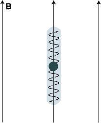
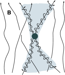
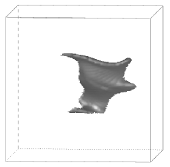
(a)	(b)	(c)

Figure 2: Models of thermal diffusion. (a) Classical picture. $\kappa_{\perp}\ll\kappa_{Sp}$. (b) Narayan & Medvedev (2001). Wandering of field lines provides efficient diffusion ($\kappa_{\perp}\sim\kappa_{Sp}/5$) in the direction perpendicular to ${\bf B}_{0}$. But, the model assumes ${\bf B}_{0}$ of $\sim$ equipartition value. (c) Turbulent diffusion model. Thermal electrons are mixed by turbulent motions, which leads to turbulent diffusion coefficient of $\kappa_{dynamic}\sim v_{turb}l_{inj}$. In many astrophysical situations, this coefficient is comparable with the Spitzer value. The figure is the snapshot of the passive scalar field at t$\sim$3 from the MHD run described in Figure 1(c); $192^{3}$ grid points, $M_{s}\sim$ 0.3, and $V_{A}=1$. In the case shown here, the mean field is strong and parallel to to the dashed line. In general, mean magnetic fields, weak or moderately strong, do not strongly suppress turbulent motions/diffusion.

References

- (1) Begelman, M. & Fabian, A. 1990, MNRAS, 244, 26
- (2) Berghöfer, T. W., Bowyer, S., Lieu, R., & Knude, J. 1998, ApJ, 500, 838
- (3) Boffetta, G., Sokolov, I. 2002, Phy. Rev. Lett., 88(9), 094501
- (4) Cho, J., Lazarian, A., Vishniac, E. 2002, ApJ, 564, 291
- (5) Fabian, A.C. 1994, ARA& A, 32, 277
- (6) Fabian, A.C., Mushotzky, R.F., Nulsen, P.E.J., & Peterson, J.R. 2001, MNRAS, 321, L20
- Goldreich & Sridhar (1995) Goldreich, P. & Sridhar, S. 1995, ApJ, 438, 763
- (8) Ishihara, T. & Kaneda, Y. 2001, APS, DFD01, BC001
- (9) Jiang, G.& Wu, C. 1999, J. Comp. Phys., 150, 561
- (10) Lazarian, A. & Vishniac, E. T. 1999, ApJ, 517, 700
- (11) Lesieur, M. 1990, Turbulence in fluids : stochastic and numerical modelling, 2nd. rev. ed. (Dordrecht; Kluwer Academic Publishers)
- (12) Liu, X. & Osher, S. 1998 J. Comp. Phys., 141, 1
- Maron & Goldreich (2001) Maron, J. & Goldreich, P. 2001, ApJ, 554, 1175
- (14) Narayan, R., & Medvedev M.V. 2001, ApJ, 562, L129
- (15) Richardson, L. F. 1926, Proc.R. Soc. London, Ser. A, 110, 709
- (16) Smith, R. & Cox, D. 2001, ApJS, 134, 283
- (17) Spitzer, L. 1962, Physics of Fully Ionized Gases (New York: Interscience)
- (18) Zakamska, N.L, & Narayan, R. 2002, astro-ph/0207127