The Reionization History at High Redshifts II: Estimating the Optical Depth to Thomson Scattering from CMB Polarization

Abstract

In light of the recent inference of a high optical depth to Thomson scattering, $\tau$, from the WMAP data we investigate the effects of extended periods of partial ionization and ask if the value of $\tau$ inferred by assuming a single sharp transition is an unbiased estimate. We construct and consider several representative ionization models and evaluate their signatures in the CMB. If $\tau$ is estimated with a single sharp transition we show that there can be a significant bias in the derived value (and therefore a bias in $\sigma_{8}$ as well). For WMAP noise levels the bias in $\tau$ is smaller than the statistical uncertainty, but for Planck or a cosmic variance limited experiment the $\tau$ bias could be much larger than the statistical uncertainties. This bias can be reduced in the ionization models we consider by fitting a slightly more complicated ionization history, such as a two-step ionization process. Assuming this two-step process we find the Planck satellite can simultaneously determine the initial redshift of reionization to $\pm 2$ and $\tau$ to $\pm 0.01$ Uncertainty about the ionization history appears to provide a limit of $\sim 0.005$ on how well $\tau$ can be estimated from CMB polarization data, much better than expected from WMAP but significantly worse than expected from cosmic-variance limits.

1. Introduction

Understanding the reionization of the intergalactic medium is important for cosmology for at least two reasons. How reionization occurred provides crucial data on the first (and possibly second) generation of sources, while Thomson scattering of the photons of the cosmic microwave background (CMB) by free electrons suppresses “primordial” anisotropies in the CMB imprinted at $z\sim 1000$.

The first sources are not well understood (see Barkana & Loeb 2001 for a recent review), but there are several relevant observational constraints. The observation of quasars at $z\sim 6$ that show strong HI absorption (Becker et al., 2001) indicates that the universe had at least 1% of the total hydrogen content in neutral form (Fan et al., 2002) at $z\sim 6$, with this neutral mass fraction rapidly decreasing at lower redshifts (Songaila & Cowie 2002). This is a strong indication that the epoch of reionization ended at $z\sim 6$. On the other hand, the observed anisotropies of the CMB indicate that the total optical depth to Thomson scattering is not extremely high, suggesting that reionization couldn’t have started at redshifts much higher than about 30 (Spergel et al., 2003).

What happened between redshifts 6 and 30 is unknown. There has been extensive modeling and numerical simulation, but without a good understanding of the sources robust conclusions are difficult to draw. Many studies have concluded that reionization should happen fairly rapidly (Cen and McDonald, 2002; Fan et al., 2002), but several recent studies have suggested (Wyithe & Loeb 2003; Cen 2003; Haiman & Holder 2003: hereafter paper I) that reionization is an extended process, perhaps even with multiple epochs of reionization.

In recent work (Kaplinghat et al. 2003; hereafter K03) it was shown that a two-step reionization process could have an observable signature in the large-angle CMB polarization anisotropies that would provide unique information on the process of reionization in this difficult-to-probe redshift range. In this work, we extend these calculations to physically motivated reionization histories provided by semi-analytic models and address the possibility that non-trivial ionization histories can introduce a bias in estimates of the optical depth $\tau$ if a simple one-step model is used to fit the data.

The results from WMAP have opened a new window on the dark ages. Several key cosmological parameters have been measured to high precision and WMAP has observed the signature of free electrons at $z\sim 10$ for the first time (Kogut et al., 2003). Previously, there had been practically no information about the ionization state of the IGM for $6.3\lesssim z\lesssim 30$.

The optical depth to Thomson scattering is an important cosmological parameter. The temperature power spectrum only allows constraints on the normalization of the primordial gravitational potential power spectrum $P_{\phi}$ in the combination $P_{\phi}e^{-2\tau}$, so a determination of $\tau$ allows a determination of the amplitude of potential (and mass) fluctuations. There has been much recent controversy over the amplitude of mass fluctuations on scales of $8h^{-1}$ Mpc, $\sigma_{8}$, as summarized in recent parameter estimates (Spergel et al., 2003). Estimates have varied by nearly a factor of two between different methods of determination within the last few years, so precise and accurate CMB estimates would be invaluable. With accurate determinations of $\sigma_{8}$ it should be possible to put strong constraints on the nature of the dark energy (Hu, 2002).

In the next section we describe the models that are used to generate a zoo of ionization histories, while § 3 demonstrates the effects of non-trivial ionization histories on CMB polarization anisotropies and parameter estimation. In § 4 we provide a crude example of how it is possible to reduce any biases induced by an unknown ionization history, and we close with a discussion.

As a fiducial model we assume cosmological parameters $\Omega_{m}=0.29$, $\Omega_{\Lambda}=0.71$, $\Omega_{b}\,h^{2}=0.024$, $h=0.72$ and an initial matter power spectrum $P(k)\propto k$ in agreement with recent results from WMAP (Spergel et al., 2003).

2. Reionization Models

We employ semi–analytical models of reionization, in order to derive a sample of physically motivated ionization histories. Details of the models are laid out in paper I, and we only briefly review the main framework here. The models assume that the total volume fraction of ionized regions is being driven by ionizing sources located in dark matter halos whose abundance is described by the N–body simulations of Jenkins et al. (2001) We distinguish dark matter halos in three different ranges of virial temperatures, as follows:

$100\,{\rm K}$  $\sim$$<$	$T_{\rm vir}$	$\;\hbox to0.0pt{\lower 2.5pt\hbox{$\sim$}\hss}\raise 1.5pt\hbox{$<$}\;10^{4}\,{\rm K}$	(Type II)
$10^{4}\,{\rm K}$  $\sim$$<$	$T_{\rm vir}$	$\;\hbox to0.0pt{\lower 2.5pt\hbox{$\sim$}\hss}\raise 1.5pt\hbox{$<$}\;2\times 10^{5}\,{\rm K}$	(Type Ia)
	$T_{\rm vir}$	$\;\hbox to0.0pt{\lower 2.5pt\hbox{$\sim$}\hss}\raise 1.5pt\hbox{$>$}\;2\times 10^{5}\,{\rm K}$	(Type Ib)

We will hereafter refer to these three different types of halos as Type II, Type Ia, and Type Ib halos. Each type of halo plays a different role in the reionization history. In short, Type II halos can host the first ionizing sources, but only in the neutral regions of the IGM, and only if ${\rm H_{2}}$ molecules are present in sufficient quantity to allow efficient cooling; Type Ia halos can only form new ionizing sources in the neutral IGM regions, but irrespective of the ${\rm H_{2}}$ abundance, and Type Ib halos can form ionizing sources regardless of the ${\rm H_{2}}$ abundance, and whether they are in the ionized or neutral phase of the IGM.

The contribution of each halo to reionization is quantified by explicitly computing the expansion of the ionized Strömgren region, dictated by the source luminosity and the background IGM density and the clumping factor $C_{\rm HII}$. We allow the three different sources above to have different efficiencies $\epsilon$ of injecting ionizing radiation into the IGM. Here $\epsilon\equiv N_{\gamma}f_{\rm esc}f_{*}$, where $f_{*}\equiv M_{*}/(\Omega_{\rm b}M_{\rm halo}/\Omega_{m})$ is the fraction of baryons in the halo that turns into stars ($\sim 10\%$ in normal stars $\;\hbox to0.0pt{\lower 2.5pt\hbox{$\sim$}\hss}\raise 1.5pt\hbox{$<$}\;0.01$ in Type II halos); $N_{\gamma}$ is the mean number of ionizing photons produced by an atom cycled through stars, averaged over the initial mass function (IMF) of the stars ($\sim 4000$ for a normal Salpeter IMF, and up to a factor of 20 higher for a population of massive, metal–free stars (Bromm, Kudritzki & Loeb 2001; Schaerer 2002); and $f_{\rm esc}$ is the fraction of these ionizing photons that escapes into the IGM ($\sim 10\%$ for Types Ia,b halos, and $\sim 1$ for Type II halos). In our models, we also allow the possibility that radiative feedback effects photo–dissociate ${\rm H_{2}}$ molecules below some critical redshift $z_{\rm uv}$, and we self–consistently exclude the Type II and Type Ia halos from forming any ionizing sources inside regions that had already been reionized. We adopt a fixed $C_{\rm HII}=10$ in all models; variations in the clumping factor can be absorbed into changes in the efficiencies with redshift.

In summary, our model has four parameters: the overall efficiencies, $\epsilon_{\rm II}$, $\epsilon_{\rm Ia}$, $\epsilon_{\rm Ib}$, and the redshift $z_{\rm uv}$ at which ${\rm H_{2}}$ dissociative feedback sets in. We here use 5 different models that are broadly representative. Three of the models were chosen to have optical depth equal to that measured by the WMAP experiment (Kogut et al., 2003) and two others were chosen to investigate the effects of larger or smaller optical depths. Details of the models can be found in paper I.

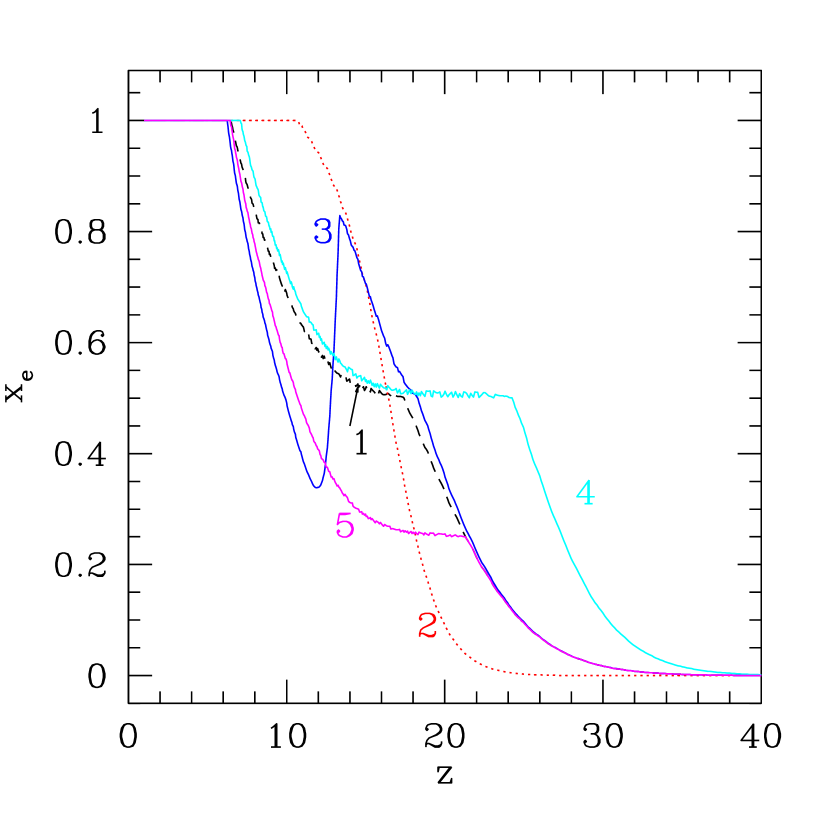
Model 1 assumes that for massive halos the stellar IMF is not metal-free (pop II) while minihalos (cooled by $H_{2}$) form metal–free stars that produce $\sim 20$ times more ionizing photons. In terms of model parameters, this corresponds to $(\epsilon_{\rm HII},\epsilon_{\rm Ia,Ib})=(200,80)$. It is assumed that $H_{2}$ starts to be destroyed at $z_{\rm uv}=17$. Model 2 assumes that minihalos do not contribute to reionization (efficient destruction of $H_{2}$) and that the efficiency in larger halos is increased to $\epsilon_{\rm Ia}\sim 4800$. In Model 3 it is assumed (as in Wyithe & Loeb 2003; Cen 2003) that there is a sharp transition from metal-free to normal stars at $z=14$. Model 4 assumes that minihalos are more effective at forming stars than in Model 1, with $\epsilon_{\rm II}=1400$ and has molecules being destroyed at $z_{\rm uv}\sim 25$. Finally, Model 5 assumes that feedback from star formation becomes efficient at destroying molecules at $z_{\rm uv}\lesssim 21$ but the same efficiencies as Model 1.

The ionization histories in our models are shown in Figure 1. As discussed in depth in paper I, the physics of reionization is rich in features that can naturally lead to distinctive ionization histories. These features can arise because of (1) the different types of coolants in halos with virial temperatures above and below $\sim 10^{4}$K, (2) the different response of different halos to radiative feedback on the ${\rm H_{2}}$ chemistry, and to photoionization feedback on gas infall, and (3) the different properties of metal–free and normal stellar populations.

In all models, we assume singly-ionized Helium traces ionized hydrogen (i.e., 1.08 free electrons per hydrogen atom for a completely ionized universe). In what follows, discussion of $x_{e}$ ignores Helium (e.g., complete ionization is referred to as $x_{e}=1$), but the factor of 1.08 is included in all calculations.

3. Large Angle CMB Polarization Anisotropies

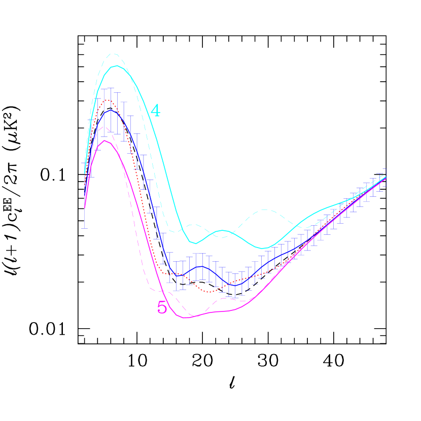
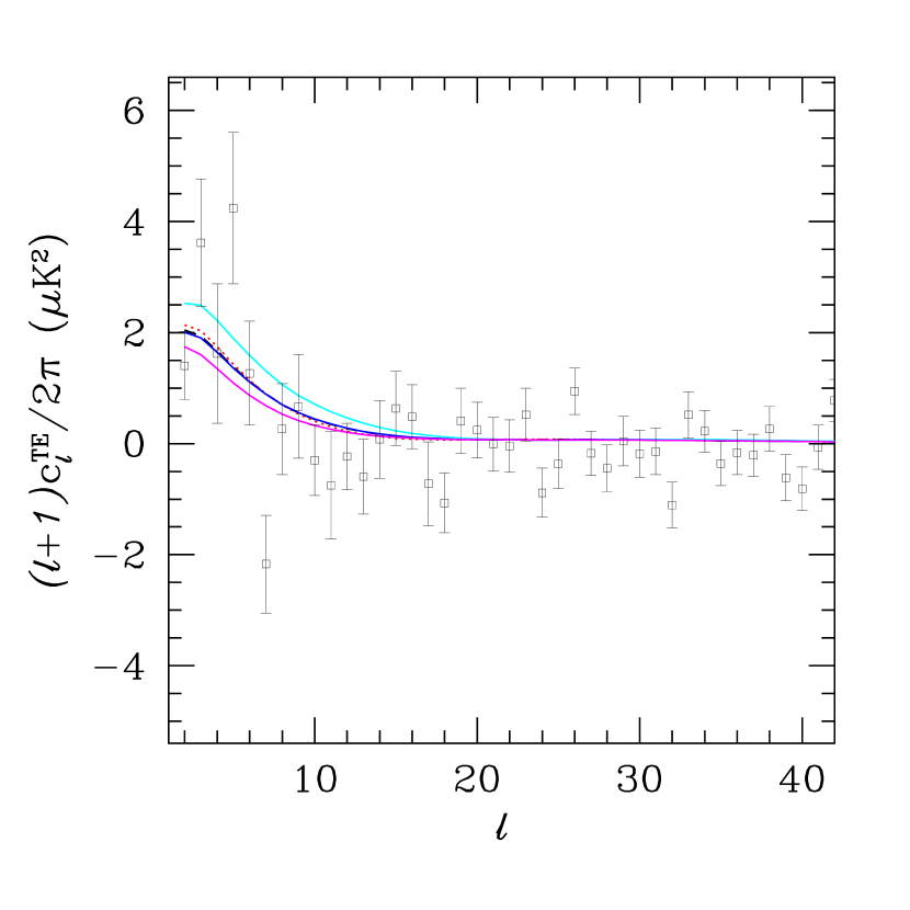
We modified CMBFast (Seljak and Zaldarriaga, 1996) to use the ionization histories from the previous section to generate temperature (TT), polarization (EE), and cross anisotropy (TE) power spectra, $C_{T\ell},C_{E\ell}$ and $C_{C\ell}$ respectively. A similar modification was done by Bruscoli, Ferrara, and Scannapieco (2002) but for an ionization history extracted from a numerical simulation, and by Naselsky and Chiang (2003) using different ionization histories. The ionization histories are shown in Figure 1 and the corresponding power spectra are shown in Figures 2 and 3.

Note in Figure 2 that for larger optical depths, there are secondary bumps in the $C_{El}$. These are thoroughly explained in Zaldarriaga (1997). For the $C_{Cl}$ (shown in Figure 3) an important difference is that we are correlating quantities which, for each value of $k$, have different angular frequencies on the sky. The polarization has angular frequency $l=k(\eta_{0}-\eta_{ri})$ (where $\eta_{0}$ and $\eta_{ri}$ are the conformal times today and at the onset of reionization) since it is projecting from the epoch of reionization where it was created. The temperature has a correspondingly higher angular frequency since it is projecting from the (further) last-scattering surface. The matched angular frequencies of $E$ correlated with $E$ lead to secondary peaks in $C_{El}$, whereas the mismatched angular frequencies of $T$ and $E$ wash out the fluctuation power and do not lead to secondary peaks in $C_{Cl}$.

As found in K03, for highly sensitive experiments approaching the cosmic-variance limit, almost all the sensitivity to $\tau$ comes from $C_{El}$. This is because $C_{El}\propto\tau^{2}$ whereas $C_{Cl}\propto\tau$ and because the fractional uncertainty in $C_{El}$ is smaller than the fractional uncertainty in $C_{Cl}$ in the cosmic variance limit. These fractional uncertainties would be equal in the limit of perfect correlation ($C_{Cl}=\sqrt{C_{El}C_{Tl}}$).

We normalize $P_{\Phi}(k=0.05{\rm Mpc}^{-1})e^{-2\tau}$ by requiring that the temperature fluctuation at $\ell=150$ is 150 $\mu K$. This choice is arbitrary, but largely irrelevant for our purposes. Varying the ionization history with this product fixed produces no change in the angular power spectra at $\ell\gtrsim 50$ (except due to non-linear effects at $\ell\gtrsim 2000$). Note that since $C_{T\ell}$ has been measured well in this range, a higher optical depth requires a larger normalization of $P_{\Phi}$ in order to agree with the data. As outlined in K03, variations in the fiducial model, such as a slight tilt or a slightly different normalization, will not have a large effect on our conclusions.

Figure 1.— Ionization histories for the five models (explained in the text) considered.

Figure 2.— Polarization power spectra for the five models (see Figure 1) considered. Model 1 is shown as a bold dashed line, model 2 is shown as a dashed line and model 3 is the solid line with cosmic variance error bars shown. Note that models 1–3 all have the same optical depth. For models 4 and 5 the best fit single transition model polarization spectra are shown as dashed lines of the same color. All models are normalized to give the same temperature power spectrum at $\ell\gtrsim 50$.

Figure 3.— Same five models as in Fig. 2 but now for the cross–correlation and with WMAP measurements plotted. As before, top line is model 4, bottom line is model 5, and models 1–3 are nearly indistinguishable.

To explore questions of bias in $\tau$ we see how well purely phenomenological models with one or two sharp transitions can be used to fit our physical models (1)-(5). For measurement uncertainties we assume Gaussian, white detector noise and ignore beam effects. We calculate the likelihood of the phenomenological models, given one of the physical models as the “data”, denoted now with a $d$ superscript (see K03):

$$\bar{\chi}^{2}\equiv-2\ln\mathcal{L}=\sum_{\ell}(2\ell+1)f_{sky}\Bigl{[}\ln([C_{E\ell}+w^{-1}]C_{T\ell}-C_{C\ell}^{2})$$

$$+{[C_{E\ell}+w^{-1}]C_{T\ell}^{d}+C_{T\ell}C_{E\ell}^{d}-2C_{C\ell}C_{C\ell}^{d}\over[C_{E\ell}+w^{-1}]C_{T\ell}-C_{C\ell}^{2}}\Bigr{]}\quad.$$ (1)

In the above, $f_{sky}$ is the fraction of sky coverage (which we take to be unity), and $w$ is the weight per unit solid angle for polarization measurements. We have assumed that for our purposes we can ignore detector noise in the measurement of the temperature power spectrum. Note that we have included the effects of all the data, i.e., EE, TT, and TE correlations are all implicitly taken into account. We have not included possible effects of foregrounds. For WMAP, we assume $w=2\times 10^{14}$, roughly the expected two-year two channel sensitivity (allowing other frequencies to be used for foreground removal) while for Planck we assume $w=1.67\times 10^{16}$, corresponding roughly to one year and two frequencies. We adopt these values as representative of the expected performance of the instruments, but should be viewed as order of magnitude estimates. For an ideal cosmic variance limited experiment $w^{-1}=0$. We require that $C_{T\ell}>0.01w^{-1}$ in the fiducial model to be included in the likelihood calculation to suppress contributions from points with low signal-to-noise.

Table 1 Best fit single-step reionizations (roughly, number of $\sigma$ is $\sqrt{\Delta\bar{\chi}^{2}}$)

			Cos. Var.				WMAP			Planck
model	$\tau$	$z_{tr}$	$\tau_{cv}$	$\Delta\bar{\chi}^{2}_{cv}$	$z_{tr}$	$\tau_{wmap}$	$\Delta\bar{\chi}^{2}_{wmap}$	$z_{tr}$	$\tau_{planck}$	$\Delta\bar{\chi}^{2}_{planck}$
1	0.169	16.3	0.166	57	16.1	0.163	0.3	16.9	0.174	15
2	0.169	16.1	0.163	9	16.3	0.166	0.0	16.3	0.166	2
3	0.169	17.0	0.176	49	16.2	0.164	0.4	17.3	0.181	16
4	0.228	20.4	0.229	112	19.6	0.216	1.1	20.9	0.238	39
5	0.139	14.4	0.138	43	13.8	0.130	0.2	14.9	0.145	13

For simplicity, we only include terms up to $\ell=50$. There is practically no information in higher multipoles, although there is likely to be some signature at $\ell\gtrsim 2000$ from non-linear effects, which could be important. We minimize this function by adjusting the transition redshift, $z_{tr}$, of a model with sudden reionization and calculate the difference in $\bar{\chi}^{2}$ of this best-fit sudden model relative to the true model. The true model is thus $\exp(\Delta\bar{\chi}^{2}/2)$ more likely than the most likely phenomenological model. For Gaussian statistics, our estimator $\bar{\chi}^{2}$ is equal to the usual $\chi^{2}$ statistic, so a rough estimate of the number of “sigmas” is $\sqrt{\Delta\bar{\chi}^{2}}$. Large values of this misfit statistic indicate that the true model is a much better fit than the model being considered while small values indicate a model that is virtually indistinguishable from the input model. The best fitting sudden models are indicated in Table 1, along with the difference in $\bar{\chi}^{2}$ and the optical depth of both the best fit and the input model. The first two columns indicate model number (see Figure 1) and true optical depth. Columns 3-5 show results of fitting a single sharp reionization assuming cosmic variance error bars and indicate the best fit single reionization redshift, best fit optical depth, and difference in $\bar{\chi}^{2}$ relative to true model. Columns 5, 6 and 7 show best fit single transition redshift, optical depth and misfit statistic assuming WMAP noise levels, while the last three columns show the same parameters assuming Planck noise levels.

For some of the models the misfit is very large, in one case a shift in the misfit statistic of more than 100 (roughly “10 $\sigma$”) for a cosmic variance limited experiment. This confirms that there is significantly more information in the large angle polarization signal than simply the optical depth, as shown in K03. For the most basic reionization signal the misfit is just above the “3 $\sigma$” level for cosmic variance limits, indicating that if reionization happens fairly quickly the exact nature of the transition is unimportant and the dominant effect on the CMB signal will be only that of the optical depth. This corresponds to the case studied by Bruscoli, Ferrara, and Scannapieco (2002), although even for this case our results are slightly less pessimistic. Part of this is due to the higher optical depth of our fiducial model, providing more signal.

From the point of view of parameter estimation, it is striking that the best fit sharp transition can provide a biased estimate of the optical depth, especially compared to the statistical uncertainties. For the assumed sensitivity of WMAP the statistical uncertainty $\delta\tau$ should be $\sim 0.02$, for Planck $\delta\tau\sim 0.005$ and for cosmic variance errors $\delta\tau\sim 0.002-0.003$. For the more exotic ionization histories the optical depth can be seen to be significantly biased for cosmic variance level measurements, with the direction and the magnitude of the bias sensitive to the details of the ionization history. Using the incorrect ionization history for model fitting introduces a systematic error in the value of $\tau$ with a direction and magnitude that depends on the details of $x_{e}(z)$. As seen in models 3 and 4, offsets between the true and derived optical depths could easily be $\gtrsim$0.01 for Planck. Determination of the optical depth, and thus the matter power spectrum amplitude, will be limited by a lack of understanding of the nature of the reionization process. For WMAP, it appears that the derived optical depth assuming a single sharp transition will not be highly biased for any of the reionization models that we consider, given that the estimated uncertainty in $\tau$ is $\sim 0.03$ (K03).

4. Toward Unbiased Optical Depth Estimates

There is information in the shape of the large angle polarization power spectra, so it is informative to see what can be gleaned. In Figure 4 we show the results of an analysis similar to that of K03. We used a simple two-step model, where it is assumed that a transition from partial ionization to full ionization occurred at $z=6.3$ and that a transition from nearly zero to an intermediate (constant) ionization fraction, $x_{e}$, occurred at $z=z_{e}$. We examine two fiducial models, one with $z_{e}=25$ and the other with $z_{e}=16$, with $x_{e}$ values chosen so that both have $\tau=0.148$. We then investigate the accuracy with which $\tau$ and $z_{e}$ can be recovered assuming noise levels typical for WMAP or expected for Planck by once again taking the fiducial model as the data and evaluating the likelihood (Eq. 1) as a function of the two parameters of the model. Figure 4 displays contours of constant likelihood for the three experimental cases. At noise levels appropriate for WMAP it will be very difficult to differentiate between different models that yield the same optical depth (as pointed out in K03 and verified by Kogut et al. 2003), but Planck would be able to determine the onset of partial reionization quite well and a cosmic variance limited experiment would be able to determine this onset very precisely. There will therefore likely be suggestions in the data itself pointing to better models for measuring $\tau$.

Figure 4.— Constant likelihood contours at 10% (thick curves) and 1% (thin curves) of the maximum likelihood – which occurs at the fiducial models labeled by A and B denoted by asterisks. A is a model completely reionized below $z=18$ and B has $z_{\rm early}=32$ and $x_{e}=0.4$; both models have $\tau=0.148$. All the panels have the same fiducial models. The solid curves correspond to model A, the dashed curves to model B. The upper panel is for a cosmic variance limited experiment (about 25 times the raw sensitivity of Planck). The middle panel assumes 1 Planck channel sensitivity while the lower panel is for two channel WMAP sensitivity.

In the previous section, we saw that the largest biases arise in the cases where the misfit statistic is also large. Therefore when the measured $\tau$ is highly biased the quality of fit will probably also be bad, indicating a possibly contaminated result. We now investigate whether a slightly more complicated fitting form for the ionization history can lead to better estimates of the optical depth. As a simple example of a path to a possibly less biased estimate of the optical depth, we fit models with a two-step reionization process, where the ionization history is characterized by a redshift of first ionization $z_{early}$, when the ionized fraction went quickly from effectively zero to $x_{e}$, and a second redshift, $z_{late}$ when the ionized fraction went quickly to unity. To ensure stability in the numerical implementation we have jumps in the ionization fraction take place over a range in redshift of $\Delta z=1$ centered on the nominal redshift of the transition and interpolated in $log(z)$. For each ionization model from the previous section, we vary the three ionization parameters to find the values that minimize the misfit statistic, assuming cosmic variance errors only.

Table 2Best fit two-step reionizations, assuming cosmic variance limited errors

model	$\tau$	$z_{late}$	$z_{early}$	$x_{e}$	$\tau_{cv}$	$\Delta\bar{\chi}^{2}_{cv}$	$\delta\tau$
1	0.169	10	24	0.45	0.172	3	$\pm$ 0.006
2	0.169	14	20	0.45	0.169	0.2	$\pm$ 0.004
3	0.169	8	23	0.55	0.171	2	$\pm$ 0.005
4	0.228	18	29	0.30	0.234	3	$\pm$ 0.008
5	0.139	3	34	0.65	0.140	2	$\pm$ 0.004

Table 2 shows the derived optical depths from fitting a two-step model. Column 2 indicates the true optical depth, the third column indicates redshift at which $x_{e}=1$ and the fourth column shows redshift at which $x_{e}$ changes from effectively zero at higher redshift to the value shown in column 5. The fifth column shows optical depth of this best fit model, while the sixth column shows the difference in $-2ln\mathcal{L}$ of this best fit relative to the true model. The final column shows the uncertainty in the determination of $\tau$ when the extra parameters are allowed in the fit. This uncertainty was determined from the smallest and largest values of $\tau$ found in models with $\Delta\bar{\chi}^{2}<1$.

As can be seen in Table 2, in this case the misfit statistics are much lower and the optical depth estimates are much less biased. In most cases the estimated values of $\tau$ are now biased at levels near or below the cosmic variance statistical errors, indicating that imperfect knowledge of the ionization history is not a fundamental limit to a good measure of $\tau$. In model 4 our two-step model may not be adequate, in that the bias in $\tau$ is comparable to the statistical uncertainty. If the measured optical depth is very high ($\gtrsim 0.2$) some care will be required to obtain a precise and accurate estimate of the amplitude of the matter power spectrum. Note that the reduction in bias has come with the cost of statistical errors in $\tau$ increasing by a factor of $~{}2$.

In general, ionization histories with widely separated (in redshift) episodes of ionization seem most prone to biased estimates of $\tau$. We have not provided an exhaustive exploration of the possible parameter space of ionization histories, so it is still possible that reionization histories exist with larger biases and/or there are cases where a two-step reionization history does little to improve estimates of $\tau$.

It is likely that there is a more physical parameterization of the ionization history that can both minimize biases in parameter estimates and provide insight into the first generation of sources. If the optical depth is measured to be higher than 0.1, as hinted by recent WMAP results, it will be important to find a good parameterization.

5. Discussion

We have shown that large angle polarization measurements could be very useful for shedding light on the end of the dark ages, a topic addressed in further detail in paper I. Conversely, it appears that at least a rudimentary understanding of the dark ages, beyond a simple optical depth to some characteristic redshift, will be required to be able to measure the amplitude of primordial fluctuations to very high accuracy. Particularly if CMB measurements suggest that the optical depth is high ($\gtrsim 0.2$), there is a real danger of mis-estimating the true optical depth by a significant amount ($>0.01$). In the near term, it appears that estimates of the optical depth based on the WMAP satellite will not be heavily biased at the level of the expected precision of 0.03 (K03). Therefore, the derived values of $\sigma_{8}$ in recent work are robust ( within the statistical uncertainties) to the choice of ionization history that is used to do the fit. This is unlikely to be the case for the next generation of instruments, given the apparently high optical depth measured by WMAP.

Allowing even a moderately more complex ionization history allows much of the bias to be removed, at the expense of larger uncertainties. Uncertainty in the ionization history appears to provide a floor of $\sim 0.005$ on how well we can measure the optical depth to Thomson scattering from CMB polarization observations.

Foreground contamination of large angle measurements is currently unknown for polarization experiments. With its extensive frequency coverage, Planck will be an exquisite instrument for characterizing and assessing the importance of astronomical sources of polarization. We believe we have been fairly conservative in our estimates of how many frequencies will be available for CMB measurement.

CMB polarization measurements provide a unique complement to absorption studies. While hydrogen absorption studies are sensitive to the fraction of neutral hydrogen, CMB polarization is sensitive to the fraction of ionized hydrogen. The signature of partial ionization at $z\sim 15$ will be very difficult to detect using absorption studies, so it will be extremely useful to have a complementary tool.

References

- Becker et al. (2001) Becker, R. H. et al. 2001, AJ, 122, 2850–2857.
- Bromm, Ferrara, Coppi, & Larson (2001) Bromm, V., Ferrara, A., Coppi, P. S., & Larson, R. B. 2001, MNRAS, 328, 969
- Bromm, Kudritzki, & Loeb (2001) Bromm, V., Kudritzki, R. P., & Loeb, A. 2001, ApJ, 552, 464
- Bruscoli, Ferrara, and Scannapieco (2002) Bruscoli, M., Ferrara, A., and Scannapieco, E. 2002, MNRAS, 330, L43–L47.
- Cen (2003) Cen, R. 2003, ApJ, submitted, astro–ph/0210473.
- Cen and McDonald (2002) Cen, R. and McDonald, P. 2002, ApJ, 570, 457–462.
- Fan et al. (2002) Fan, X., Narayanan, V. K., Strauss, M. A., White, R. L., Becker, R. H., Pentericci, L., and Rix, H. 2002, AJ, 123, 1247–1257.
- Haiman and Holder (2003) Haiman, Z., & Holder, G. P. 2003, ApJ, submitted
- Hu (2002) Hu, W. 2002, Phys. Rev. D, 66, 83515
- Jenkins et al. (2001) Jenkins, A., Frenk, C. S., White, S. D. M., Colberg, J. M., Cole, S., Evrard, A. E., Couchman, H. M. P., and Yoshida, N. 2001, MNRAS, 321, 372.
- Kaplinghat et al. (2003) Kaplinghat, M., Chu, M., Haiman, Z., Holder, G. P., Knox, L., and Skordis, C. 2003, ApJ, 583, 24–32.
- Kogut et al. (2003) Kogut, A. et al. 2003, ApJ, submitted, astro-ph/0302213
- Loeb and Barkana (2001) Loeb, A. and Barkana, R. 2001, ARA&A, 39, 19–66.
- Naselsky and Chiang (2003) Naselsky, P. and Chiang, L.-Y. 2003, MNRAS, submitted, astro-ph/0302085
- Schaerer (2002) Schaerer, D. 2002, A&A, 382, 28
- Seljak and Zaldarriaga (1996) Seljak, U. and Zaldarriaga, M. 1996, ApJ, 469, 437
- Songaila & Cowie (2002) Songaila, A., & Cowie, L.L. 2002, AJ, 123, 2183
- Spergel et al. (2003) Spergel, D. N. et al. 2003, ApJ, submitted, astro-ph/0302209
- Wyithe and Loeb (2003) Wyithe, S. and Loeb, A. 2003, ApJ, submitted, astro–ph/0209056.
- Zaldarriaga (1997) Zaldarriaga, M. 1997, Phys. Rev. D, 55, 1822