Current constraints on Cosmological Parameters from Microwave Background Anisotropies.

Abstract

We compare the latest observations of Cosmic Microwave Background (CMB) Anisotropies with the theoretical predictions of the standard scenario of structure formation. Assuming a primordial power spectrum of adiabatic perturbations we found that the total energy density is constrained to be $\Omega_{tot}=1.03\pm 0.06$ while the energy density in baryon and Cold Dark Matter (CDM) are $\Omega_{b}h^{2}=0.021\pm 0.003$ and $\Omega_{cdm}h^{2}=0.12\pm 0.02$, (all at $68\%$ C.L.) respectively. The primordial spectrum is consistent with scale invariance, ($n_{s}=0.97\pm 0.04$) and the age of the universe is $t_{0}=14.6\pm 0.9$ Gyrs. Adding informations from Large Scale Structure and Supernovae, we found a strong evidence for a cosmological constant $\Omega_{\Lambda}=0.70_{-0.05}^{+0.07}$ and a value of the Hubble parameter $h=0.69\pm 0.07$. Restricting this combined analysis to flat universes, we put constraints on possible ’extensions’ of the standard scenario. A gravity waves contribution to the quadrupole anisotropy is limited to be $r\leq 0.42$ ($95\%$ c.l.). A constant equation of state for the dark energy component is bound to be $w_{Q}\leq-0.74$ ($95\%$ c.l.). We constrain the effective relativistic degrees of freedom $N_{\nu}\leq 6.2$ and the neutrino chemical potential $-0.01\leq\xi_{e}\leq 0.18$ and $|\xi_{\mu,\tau}|\leq 2.3$ (massless neutrinos).

]

I Introduction

The last years have been an exciting period for the field of the CMB research. With recent CMB balloon-borne and ground-based experiments we are entering a new era of ’precision’ cosmology that enables us to use the CMB anisotropy measurements to constrain the cosmological parameters and the underlying theoretical models. With the TOCO$-97/98$ ([64],[51]) and BOOMERanG-$97$ ([45]) experiments a firm detection of a first peak on about degree scales has been obtained. In the framework of adiabatic Cold Dark Matter (CDM) models, the position, amplitude and width of this peak provide strong supporting evidence for the inflationary predictions of a low curvature (flat) universe and a scale-invariant primordial spectrum ([19], [48], [62]).

The new experimental data from BOOMERanG LDB ([53]), DASI ([30]), MAXIMA ([41]), CBI ([57]), VSA ([60]) and, more recently, ACBAR ([8]), ARCHEOPS ([4]) and revised and improved analysis from BOOMERanG ([10]) and VSA ([9]) have provided further evidence for the presence of the first peak and refined the data at larger multipole (see e.g. [54]). The combined data suggest the presence of a second and third peak in the spectrum, confirming the model prediction of acoustic oscillations in the primeval plasma and sheding new light on various cosmological and inflationary parameters ([7], [65], [59]) .

In this Rapid Communication we compare the latest measurements of the Cosmic Microwave Background Anisotropies angular power spectrum with the theoretical predictions of the standard CDM scenario in order to constrain most of its parameters.

Similar and careful analysis have been done recently ([43], [57], [50]), the work presented here can be considered as a last-minute update of most of the results already published but it will also differ for following aspects: First of all, we will include the new ARCHEOPS, ACBAR, BOOMERanG and VSAE datasets, which provide the best determination to the date of region in the spectrum from the scales sample to COBE up to the Silk damping scales.

Second, we will also focus on possible deviations to the standard scenario, like gravity waves, an equation of state for the dark energy $w_{Q}>-1$ or an extra-background of relativistic particles.

Our paper is then organized as follows: In section II we present the analysis method we used. In Section III we report our results. In Section IV we discuss our conclusions.

II Method

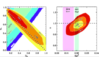
FIG. 1.: Confidence contours in the $\Omega_{M}-\Omega_{\Lambda}$ (left) and $\Omega_{b}h^{2}-n$ (Right) planes from the analysis described in the text.

As a first step, we consider a template of adiabatic, $\Lambda$-CDM models computed with CMBFAST ([61]), sampling the various parameters as follows: the physical density in cold dark matter $\Omega_{cdm}h^{2}\equiv\omega_{cdm}=0.01,...0.40$, in steps of $0.01$; the physical density in baryons $\Omega_{b}h^{2}\equiv\omega_{b}=0.001,...,0.040$, in steps of $0.001$, the cosmological constant $\Omega_{\Lambda}=0.0,...,0.95$, in steps of $0.05$ and the curvature $\Omega_{k}=-0.5,....0.5$ step $0.05$. The value of the Hubble constant is not an independent parameter, since:

$$h=\sqrt{{\omega_{cdm}+\omega_{b}}\over{1-\Omega_{\Lambda}-\Omega_{k}}}.$$ (1)

We allow for a reionization of the intergalactic medium by varying also the compton optical depth parameter $\tau_{c}$ in the range $\tau_{c}=0.0,...,0.45$ in steps of $0.05$ .

We also vary the scalar spectral index of primordial fluctuations in the range $n_{S}=0.7,...,1.3$ in steps of $0.02$.

We will then restrict our analysis to flat models and, adding external priors as described below, we will constrain possible extensions of the standard model. In particular, we will consider a background of gravity waves, parametrized as a contribution to the CMB anisotropy quadrupole $r=C_{2}^{T}/C_{2}^{S}$. We consider the tensor spectral index $n_{T}$ to be $n_{T}=-r/6.8$ for $n_{S}<1$ and $n_{T}=0$ for $n_{S}>1$.

We will also consider an equation of state for the dark energy $w_{Q}\neq-1$ sampled as $w_{Q}=-1.0,...,-0.4$ in step of $0.05$. Finally we will constrain an extra-background of relativistic particles, parametrized through an effective number of relativistic neutrinos $\Delta N^{eff}$ sampled as $\Delta N^{eff}=0.0,...,10.0$ in step of $0.5$.

For the CMB data, we use the recent results from the BOOMERanG-98, DASI, MAXIMA-1, CBI, VSAE, ACBAR and ARCHEOPS experiments. Where possible, we use the publicly available window functions and offset lognormal correction prefactors $x_{b}$ in order to compute the theoretical band power signal $C_{B}$ as in [12]. The likelihood for a given theoretical model is defined by $-2{\rm ln}{\cal L}=(C_{B}^{th}-C_{B}^{ex})M_{BB^{\prime}}(C_{B^{\prime}}^{th}-C_{B^{\prime}}^{ex})$ where $M_{BB^{\prime}}$ is the Gaussian curvature of the likelihood matrix at the peak.

We include the beam and calibration uncertainties by the marginalization methods presented in ([11], see also [69]).

In addition to the CMB data we will also consider the real-space power spectrum of galaxies in the 2dF 100k galaxy redshift survey using the data and window functions of the analysis of Tegmark et al. ([63]).

To compute ${\cal L}^{2dF}$, we evaluate $p_{i}=P(k_{i})$, where $P(k)$ is the theoretical matter power spectrum and $k_{i}$ are the $49$ k-values of the measurements in [63]. Therefore we have $-2ln{\cal L}^{2dF}=\sum_{i}[P_{i}-(Wp)_{i}]^{2}/dP_{i}^{2}$, where $P_{i}$ and $dP_{i}$ are the measurements and corresponding error bars and $W$ is the reported $27\times 49$ window matrix. We restrict the analysis to a range of scales where the fluctuations are assumed to be in the linear regime ($k<0.2h^{-1}\rm Mpc$). When combining with the CMB data, we marginalize over a bias $b$ considered to be an additional free parameter.

Furthermore, we will also incorporate constraints obtained from the luminosity measurements of type I-a supernovae (SN-Ia). The observed apparent bolometric luminosity is related to the luminosity distance, measured in Mpc, by $m_{B}=M+5logd_{L}(z)+25$. where M is the absolute bolometric magnitude. The luminosity distance is sensitive to the cosmological evolution through an integral dependence on the Hubble factor $d_{l}=(1+z)\int_{0}^{z}(dz^{\prime}/H(z^{\prime},\Omega_{Q},\Omega_{M},w_{q})$ where $\Omega_{Q}$ and $w_{Q}$ are the energy density and equation of state of the “dark energy” component. We evaluate the likelihoods assuming a constant equation of state, such that $H(z)=\rho_{0}\sum_{i}\Omega_{i}(1+z)^{(3+3w_{i})}$. The predicted $m_{eff}$ is then calculated by calibration with low-z supernovae observations where the Hubble relation $d_{l}\approx H_{0}cz$ is obeyed. We calculate the likelihood, ${\cal L}$, using the relation ${\cal L}={\cal L}_{0}\exp(-\chi^{2}(\Omega_{Q},\Omega_{M},w_{Q})/2)$ where ${\cal L}_{0}$ is an arbitrary normalisation and $\chi^{2}$ is evaluated using the observations of ([26]), marginalising over $H_{0}$.

Finally, we will also consider a $1-\sigma$ contraint on the Hubble parameter, $h=0.71\pm 0.07$, derived from Hubble Space Telescope (HST) measurements ([25]).

In order to constrain a parameter $x$ we marginalize over the values of the other parameters $\vec{y}$. This yields the marginalized likelihood distribution

$${\cal L}(x){\equiv}P({x}|\vec{\cal C}_{B})=\int{\cal L}(x,\vec{y})d\vec{y}.$$ (2)

The central values and $1\sigma$ limits are then found from the 16%, 50% and 84% integrals of $\mathcal{L}(x)$.

III Results: Standard Parameters

In Fig. $1$ we plot the likelihood contours on the $\Omega_{M}-\Omega_{\Lambda}$ and $\Omega_{b}h^{2}-n_{S}$ planes, using only the CMB data.

As we can see from Figure $1$ (Left Panel) the data strongly suggest a flat universe (i.e. $\Omega=\Omega_{M}+\Omega_{\Lambda}=1$). From our CMB dataset we obtain $\Omega=1.03\pm 0.06$ at $95\%$ C.L..

The inclusion of complementary datasets in the analysis breaks the angular diameter distance degeneracy and provides evidence for a cosmological constant at high significance. Adding the HST constraint, the 2dF dataset and SN-Ia gives $\Omega_{\Lambda}=0.67_{-0.13}^{+0.07}$, $\Omega_{\Lambda}=0.63_{-0.09}^{+0.11}$ and $\Omega_{\Lambda}=0.70_{-0.05}^{+0.07}$, all at $68\%$ c.l..

Combining CMB and 2dF gives $h=0.69\pm 0.07$ in extremely good agreement with the HST result.

In the right panel of Fig.1 we plot the CMB likelihood contours in the $\Omega_{b}h^{2}-n_{S}$ plane. As we can see, the present CMB data is in beautiful agreement with both a nearly scale invariant spectrum of primordial fluctuations, as predicted by inflation, and the value for the baryon density $\omega_{b}=0.020\pm 0.002$ ($95\%$ C.L.) predicted by Standard Big Bang Nucleosynthesis (see e.g. [13]) from measurements of primordial deuterium. For the scalar spectral index, we found: $n_{s}=0.97\pm 0.04$. However, the CMB constraint is also in agreement in between $2-\sigma$ with the lower BBN value $0.006<\Omega_{b}h^{2}<0.017$ obtained from measurements of ${}^{4}He$ and ${}^{7}Li$ ([14]) at $95\%$ C.lL..

An increase in the optical depth $\tau_{c}$ after recombination by reionization (see e.g. [29] for a review) or by some more exotic mechanism damps the amplitude of the CMB peaks. Degeneracies with other parameters such as $n_{S}$ are present (see e.g. [5]) and we cannot strongly bound the value of $\tau_{c}$. In the range of parameters we considered we have $\tau_{c}\leq 0.24$ at $1-\sigma$.

The amount of non-baryonic dark matter is also constrained by the CMB data with $\Omega_{dm}h^{2}=0.12\pm 0.02$ at $68\%$ c.l.. The presence of power around the third peak is crucial in this sense, since it cannot be easily accommodated in models based on just baryonic matter (see e.g. [50], [28], [47] and references therein).

Furthermore, under the assumption of flatness, we can derive important constraints on the age of the universe $t_{0}$. From our cmb dataset we obtain $t_{0}=14.6\pm 0.9$ GYrs consistent with the analyses of ([23], [53], [40]).

IV Results: Beyond the Standard Model.

As discussed before, even if the present CMB observations can be fitted with just $5$ parameters it is interesting to extend the analysis to other parameters allowed by the theory. Here we will just consider a few of them.

Gravity Waves.

The metric perturbations created during inflation belong to two types: scalar perturbations, which couple to the stress-energy of matter in the universe and form the “seeds” for structure formation and tensor perturbations, also known as gravitational wave perturbations. Both scalar and tensor perturbations contribute to CMB anisotropy. In most of the recent CMB analysis the tensor modes have been neglected, even though a sizable background of gravity waves is expected in most of the inflationary scenarios. Furthermore, in the simplest models, a detection of the GW background can provide information on the second derivative of the inflaton potential and shed light on the physics at $\sim 10^{16}Gev$ (see e.g. [36]).

The shape of the $C^{T}_{\ell}$ spectrum from tensor modes is drastically different from the one expected from scalar fluctuations, affecting only large angular scales (see e.g. [15]). The effect of including tensor modes is similar to just a rescaling of the degree-scale $COBE$ normalization and/or a removal of the corresponding data points from the analysis.

This further increases the degeneracies among cosmological parameters, affecting mainly the estimates of the baryon and cold dark matter densities and the scalar spectral index $n_{S}$ ([49],[38], [65], [20]).

The amplitude of the GW background is therefore weakly constrained by the CMB data alone, however, when information from galaxy clustering and SN-Ia are included, an upper limit on $r$ can be obtained.

In Fig.2 we plot the contraints obtained in the $n_{S}-r$ plane under the assumption of flatness and including the 2dF and SN-Ia data. As we can see, the possibility of a tensor component is still in agreement with the combined analysis of these datasets. Including a conservative BBN constraint $\omega_{b}<0.024$ further improves the bound to $r\leq 0.42$ at $95\%$ c.l.. Similar bounds have been found in a previous analysis ([55]), without the VSAE, ACBAR and Boomerang revised datasets.

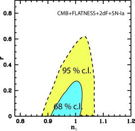
FIG. 2.: The $68\%$ and $95\%$ CL contours for the gravity waves contribution in the $n_{S}-r=C_{2}^{T}/C_{2}^{S}$ plane.

Quintessence.

The discovery that the universe’s evolution may be dominated by an effective cosmological constant [26] is one of the most remarkable cosmological findings of recent years. One candidate that could possibly explain the observations is a dynamical scalar “quintessence” field. The common characteristic of quintessence models is that their equations of state, $w_{Q}=p/\rho$, vary with time while a cosmological constant remains fixed at $w_{Q=\Lambda}=-1$. Observationally distinguishing a time variation in the equation of state or finding $w_{Q}$ different from $-1$ will therefore be a success for the quintessential scenario. Quintessence can also affect the CMB by acting as an additional energy component with a characteristic viscosity. However any early-universe imprint of quintessence is strongly constrained by Big Bang Nucleosynthesis with $\Omega_{Q}(MeV)<0.045$ at $2\sigma$ for temperatures near $T\sim 1Mev$ ([2]).

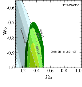
FIG. 3.: The likelihood contours in the ($\Omega_{M}$, $w_{Q}$) plane, with the remaining parameters taking their best-fitting values for the joint CMB+SN-Ia+2dF+HST analysis described in the text. The contours correspond to the 68%, 95% and 99% confidence levels respectively.

In Figure 3 we plot the likelihood contours in the ($\Omega_{M}$, $w_{Q}$) plane from our joint analyses of CMB+SN-Ia+HST+2dF together with the contours from the SN-Ia dataset only. The new CMB results improve the constraints from previous and similar analysis (see e.g., [58]), [3], [52]) with $w_{Q}<-0.87$ at $68\%$ c.l.. The current constraints are then perfectly in agreement with the $w_{Q}=-1$ cosmological constant case and gives no support to a quintessential field scenario with $w_{Q}>-1$.

In our analysis we only consider the case of a constant-with-redshift $w_{Q}$. The assumption of a constant $w_{Q}$ is based on several considerations: first of all, since both the luminosities and angular distances (that are the fundamental cosmological observables) depend on $w_{Q}$ through multiple integrals, they are not particularly sensitive to variations of $w_{Q}$ with redshift. Therefore, with current data, no strong constraints can be placed on the redshift-dependence of $w_{Q}$. Second, for most of the dynamical models on the market, the assumption of a piecewise-constant equation of state is a good approximation for an unbiased determination of the effective equation of state

$$w_{\rm eff}\sim\frac{\int w_{Q}(a)\Omega_{Q}(a)da}{\int\Omega_{Q}(a)da}$$ (3)

predicted by the model. Hence, if the present data is compatible with a constant $w_{Q}=-1$, it may not be possible to discriminate between a cosmological constant and a dynamical dark energy model.

However one should be be very careful about drawing definitive conclusions about dark energy, since a constant equation of state is still an approximation of a real model of dark energy (see e.g. [70]). The analysis presented here should be therefore regarded as a ’test’ for deviations from the cosmological constant scenario.

Big Bang Nucleosynthesis and Neutrinos.

As we saw in the previous section, the SBBN $95\%$ CL region, corresponding to $\Omega_{b}h^{2}=0.020{\pm}0.002$ ($95\%$ c.l.) (High BBN) and $0.006<\Omega_{b}h^{2}<0.017$ (Low BBN), have a large overlap with the analogous CMBR contour. This fact, if it will be confirmed by future experiments on CMB anisotropies, can be seen as one of the greatest success, up to now, of the standard hot big bang model.

SBBN is well known to provide strong bounds on the number of relativistic species $N_{\nu}$. On the other hand, Degenerate BBN (DBBN), first analyzed in Ref. [18, 24, 37], gives very weak constraint on the effective number of massless neutrinos, since an increase in $N_{\nu}$ can be compensated by a change in both the chemical potential of the electron neutrino, $\mu_{\nu_{e}}=\xi_{e}T$, and $\Omega_{b}h^{2}$. Practically, SBBN relies on the theoretical assumption that background neutrinos have negligible chemical potential, just like their charged lepton partners. Even though this hypothesis is perfectly justified by Occam razor, models have been proposed in the literature [1, 16, 17, 46], where large neutrino chemical potentials can be generated.

Combining the DBBN scenario with the bound on baryonic and radiation densities allowed by CMBR data, it is possible to obtain strong constraints on the parameters of the model. Such an analysis was, for example, performed in ([22], [42], [32], [56]) using the first data release of BOOMERanG and MAXIMA ([6], [31]).

We recall that the neutrino chemical potentials contribute to the total neutrino effective degrees of freedom $N_{\nu}$ as

$$N_{{\nu}}=3+\Sigma_{\alpha}\left[\frac{30}{7}\left(\frac{\xi_{\alpha}}{\pi}\right)^{2}+\frac{15}{7}\left(\frac{\xi_{\alpha}}{\pi}\right)^{4}\right]\,.$$ (4)

Notice that in order to get a bound on $\xi_{\alpha}$ we have here assumed that all relativistic degrees of freedom, other than photons, are given by three (possibly) degenerate active neutrinos.

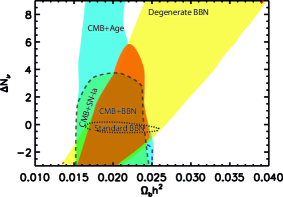
FIG. 4.: The $95\%$ CL contours for degenerate BBN, the CMB results with just the age prior, combined with SN-Ia and combined with BBN degenerate.

Figure 4 summarizes the main results with the new CMB data for the DBBN scenario (see caption). We plot the $95\%$ CL contours allowed by DBBN together with the analogous $95\%$ CL region coming from the CMB data analysis, with only weak age prior, $t_{0}>11$gyr and the $95\%$ CL region of the joint product distribution ${\cal L}\equiv{\cal L}_{DBBN}$${\cdot}{\cal L}_{CMB}$.

We obtain the bound $N_{\nu}\leq 8.4$, at $95\%$ CL, which translates into the bounds $-0.01\leq\xi_{e}\leq 0.24$, sensibly more stringent than what can be found from DBBN alone. Combining CMBR and DBBN data with the Supernova Ia data [26] strongly reduces the degeneracy between $\Omega_{m}$ and $\Omega_{\Lambda}$. At $95\%$ C.L. we find $\Delta N_{\nu}<6.2$, corresponding to $-0.01\leq\xi_{e}\leq 0.18$ and $|\xi_{\mu,\tau}|\leq 2.3$.

It is however important to note that possible extra relativistic degrees of freedom, like light sterile neutrinos, would contribute to $N_{\nu}$ as well, and in this respect BBN cannot distinguish between their contribution to the total universe expansion rate and the one due to neutrino degeneracy. Therefore, in a more general framework, our estimates for $N_{\nu}$ can only represent an upper bound for the total neutrino chemical potentials.

Similar results have been obtained in [35], [39] and [33].

V Conclusions

The recent CMB data represent a beautiful success for the standard cosmological model. Furthermore, when constraints on cosmological parameters are derived under the assumption of adiabatic primordial perturbations their values are in agreement with the predictions of the theory and/or with independent observations.

As we saw in the previous section modifications as gravity waves, quintessence or extra background of relativistic particles are still compatible with current CMB observations, but are not necessary and can be reasonably constrained when complementary datasets are included.

Since the inflationary scenario is in agreement with the data and all the most relevant parameters are starting to be constrained within a few percent accuracy, the CMB is becoming a wonderful laboratory for investigating the possibilities of new physics. With the promise of large data sets from Map, Planck and SNAP satellites and from the SLOAN digital sky survey, opportunities may be open, for example, to constrain dark energy models, variations in fundamental constants and neutrino physics.

Acknowledgements

We wish to thank Rachel Bean, Ruth Durrer, Steen Hansen, Pedro Ferreira, Mike Hobson, Will Kinney, Anthony Lasenby, Gianpiero Mangano, Gennaro Miele, Ofelia Pisanti, Antonio Riotto, Graca Rocha, Joe Silk, and Roberto Trotta for comments, discussions and help.

REFERENCES

- [1] I. Affleck and M. Dine, Nucl. Phys. B249 (1985) 361.
- [2] R. Bean, S. H. Hansen and A. Melchiorri, Phys. Rev. D 64 (2001) 103508 [arXiv:astro-ph/0104162].
- [3] R. Bean and A. Melchiorri, arXiv:astro-ph/0110472, Phys. Rev. D Rapid Communication, in press.
- [4] A. Benoit et al. [Acheops Collaboration], A & A, submitted, 2002.
- [5] P. de Bernardis, A. Balbi, G. De Gasperis, A. Melchiorri and N. Vittorio, arXiv:astro-ph/9609154.
- [6] P. de Bernardis et al. [Boomerang Collaboration], Nature 404, 955 (2000) [arXiv:astro-ph/0004404].
- [7] P. de Bernardis et al., [Boomerang Collaboration], arXiv:astro-ph/0105296.
- [8] C. l. Kuo et al., arXiv:astro-ph/0212289.
- [9] K. Grainge et al., arXiv:astro-ph/0212495.
- [10] J. E. Ruhl et al., arXiv:astro-ph/0212229.
- [11] S. L. Bridle, R. Crittenden, A. Melchiorri, M. P. Hobson, R. Kneissl and A. N. Lasenby, arXiv:astro-ph/0112114.
- [12] J. R. Bond, A. H. Jaffe and L. E. Knox, Astrophys. J. 533 (2000) 19 [arXiv:astro-ph/9808264].
- [13] S. Burles, K. M. Nollett and M. S. Turner, Astrophys. J. 552, L1 (2001) [arXiv:astro-ph/0010171].
- [14] R. H. Cyburt, B. D. Fields and K. A. Olive, New Astron. 6 (1996) 215 [arXiv:astro-ph/0102179].
- [15] R. Crittenden, J. R. Bond, R. L. Davis, G. Efstathiou and P. J. Steinhardt, Phys. Rev. Lett. 71 (1993) 324[arXiv:astro-ph/9303014].
- [16] A.D. Dolgov and D.P. Kirilova, J. Moscow Phys. Soc. 1 (1991) 217.
- [17] A.D. Dolgov, Phys. Rep.222 (1992) 309.
- [18] A.G. Doroshkevich, I.D. Novikov, R.A. Sunaiev, Y.B. Zeldovich, in Highlights of Astronomy, de Jager ed., (1971) p. 318.
- [19] S. Dodelson and L. Knox, Phys. Rev. Lett. 84, 3523 (2000) [arXiv:astro-ph/9909454].
- [20] G. Efstathiou, astro-ph/0109151.
- [21] G. Efstathiou & J.R. Bond [astro-ph/9807103].
- [22] S. Esposito, G. Mangano, A. Melchiorri, G. Miele and O. Pisanti, Phys. Rev. D 63 (2001) 043004 [arXiv:astro-ph/0007419].
- [23] I. Ferreras, A. Melchiorri and J. Silk, MNRAS 327, L47 (2001), arXiv:astro-ph/0105384.
- [24] W.A. Fowler, Accademia Nazionale dei Lincei, Roma 157 (1971) 115.
- [25] W. Freedman et al., Astrophysical Journal, 553, 2001, 47.
- [26] P.M. Garnavich et al, Ap.J. Letters 493, L53-57 (1998); S. Perlmutter et al, Ap. J. 483, 565 (1997); S. Perlmutter et al (The Supernova Cosmology Project), Nature 391 51 (1998); A.G. Riess et al, Ap. J. 116, 1009 (1998);
- [27] N. Gnedin, astro-ph/0110290.
- [28] L. M. Griffiths, A. Melchiorri and J. Silk, Astrophys. J. 553 (2001) L5 [arXiv:astro-ph/0101413].
- [29] Z. Haiman and L. Knox, arXiv:astro-ph/9902311.
- [30] N. W. Halverson et al., arXiv:astro-ph/0104489.
- [31] S. Hanany et al., Astrophys. J. 545, L5 (2000) [arXiv:astro-ph/0005123].
- [32] S. Hannestad, Phys. Rev. Lett. 85 (2000) 4203 [arXiv:astro-ph/0005018].
- [33] S. Hannestad, Phys. Rev. D 64 (2001) 083002 [arXiv:astro-ph/0105220].
- [34] S.H. Hansen and F.L. Villante, Phys. Lett. B486 (2000) 1.
- [35] S. H. Hansen, G. Mangano, A. Melchiorri, G. Miele and O. Pisanti, Phys. Rev. D 65 (2002) 023511 [arXiv:astro-ph/0105385].
- [36] M. B. Hoffman, M. S. Turner, Phys.Rev. D64 (2001) 023506, astro-ph/0006312.
- [37] H. Kang and G. Steigman, Nucl. Phys. B372 (1992) 494.
- [38] W. H. Kinney, A. Melchiorri and A. Riotto, Phys. Rev. D 63 (2001) 023505[arXiv:astro-ph/0007375].
- [39] J. P. Kneller, R. J. Scherrer, G. Steigman and T. P. Walker, Phys. Rev. D 64 (2001) 123506 [arXiv:astro-ph/0101386].
- [40] L. Knox, N. Christensen, C. Skordis, [arXiv:astro-ph/0109232].
- [41] A. T. Lee et al., Astrophys. J. 561 (2001) L1 [arXiv:astro-ph/0104459].
- [42] J. Lesgourgues and M. Peloso, Phys. Rev. D 62 (2000) 081301 [arXiv:astro-ph/0004412].
- [43] A. Lewis and S. Bridle, ” arXiv:astro-ph/0205436.
- [44] E. Lisi, S. Sarkar, and F.L. Villante, Phys. Rev. D59 (1999) 123520.
- [45] P. D. Mauskopf et al. [Boomerang Collaboration], Astrophys. J. 536, L59 (2000) [arXiv:astro-ph/9911444].
- [46] J.McDonald, Phys. Rev. Lett. 84 (2000) 4798.
- [47] S. S. McGaugh, Astrophys. J. 541 (2000) L33 [arXiv:astro-ph/0008188].
- [48] A. Melchiorri et al. [Boomerang Collaboration], Astrophys. J. 536 (2000) L63 [arXiv:astro-ph/9911445].
- [49] A. Melchiorri, M. V. Sazhin, V. V. Shulga and N. Vittorio, Astrophys. J. 518 (1999) 562, [arXiv:astro-ph/9901220].
- [50] A. Melchiorri and J. Silk, arXiv:astro-ph/0203200.
- [51] A. D. Miller et al., Astrophys. J. 524, L1 (1999) [arXiv:astro-ph/9906421].
- [52] S. Hannestad and E. Mortsell, Phys. Rev. D 66 (2002) 063508 [arXiv:astro-ph/0205096].
- [53] C. B. Netterfield et al. [Boomerang Collaboration], arXiv:astro-ph/0104460.
- [54] C. J. Odman, A. Melchiorri, M. P. Hobson and A. N. Lasenby, arXiv:astro-ph/0207286.
- [55] A. Melchiorri, C. J. Odman, astro-ph/0210606, PRD in press (2002).
- [56] M. Orito, T. Kajino, G. J. Mathews and R. N. Boyd, arXiv:astro-ph/0005446.
- [57] T. J. Pearson et al., astro-ph/0205388, (2002).
- [58] S. Perlmutter, M.S. Turner, M. White, Phys.Rev.Lett. 83 670-673 (1999).
- [59] C. Pryke, N. W. Halverson, E. M. Leitch, J. Kovac, J. E. Carlstrom, W. L. Holzapfel and M. Dragovan, arXiv:astro-ph/0104490.
- [60] P. F. Scott et al., astro-ph/0205380, (2002).
- [61] U. Seljak, M. Zaldarriaga, M. 1996, ApJ, 469, 437.
- [62] M. Tegmark, Astrophys. J. 514, L69 (1999) [arXiv:astro-ph/9809201].
- [63] M. Tegmark, A. J. S. Hamilton, Y. Xu, astro-ph/0111575 (2001)
- [64] E. Torbet et al., Astrophys. J. 521, L79 (1999) [arXiv:astro-ph/9905100].
- [65] X. Wang, M. Tegmark, M. Zaldarriaga, astro-ph/0105091.
- [66] S. Podariu et al., Astrophys.J. 559 (2001) 9
- [67] C. Miller et al., astro-ph/0112049 (2001).
- [68] A. Jaffe et al., Phys.Rev.Lett. 86 (2001) 3475-3479.
- [69] Ganga K., Ratra B., Gundersen, J., Sugyiama, N. 1997, ApJ, 484, 7.
- [70] P.J.E. Peebles, B. Ratra, astro-ph/0207347.