Galaxies as Fluctuations in the Ionizing Background Radiation at Low Redshift

Abstract

Some Lyman continuum photons are likely to escape from most galaxies, and these can play an important role in ionizing gas around and between galaxies, including gas that gives rise to Lyman alpha absorption. Thus the gas surrounding galaxies and in the intergalactic medium will be exposed to varying amounts of ionizing radiation depending upon the distances, orientations, and luminosities of any nearby galaxies. The ionizing background can be recalculated at any point within a simulation by adding the flux from the galaxies to a uniform quasar contribution. Normal galaxies are found to almost always make some contribution to the ionizing background radiation at redshift zero, as seen by absorbers and at random points in space. Assuming that $\sim 2$ percent of ionizing photons escape from a galaxy like the Milky Way, we find that normal galaxies make a contribution of at least 30 to 40 percent of the assumed quasar background. Lyman alpha absorbers with a wide range of neutral column densities are found to be exposed to a wide range of ionization rates, although the distribution of photoionization rates for absorbers is found to be strongly peaked. On average, less highly ionized absorbers are found to arise farther from luminous galaxies, while local fluctuations in the ionization rate are seen around galaxies having a wide range of properties.

1 Introduction

The extragalactic background of Lyman continuum photons plays an important role in ionizing the many absorption line systems seen shortward of Ly$\alpha$ emission in quasar spectra, including those seen at low redshifts using the ultraviolet capabilities of the Hubble Space Telescope (Bahcall et al. 1996). The ionizing background intensity determines the neutral gas fraction in Ly$\alpha$ forest absorbers and the ion ratios seen in metal absorption line systems. Furthermore, understanding the ionizing background is important for developing theories for the formation and evolution of galaxies and the Ly$\alpha$ forest and possibly for finding the baryonic mass contained within galaxies and the intergalactic medium. Interesting questions remain as to how much of this background is contributed by galaxies and what role galaxies play in ionizing gas around and between them that is detected as Ly$\alpha$ absorption.

The only largely neutral Ly$\alpha$ absorbers are the damped systems which have neutral hydrogen column densities $N_{HI}>10^{20.3}$ cm^-2. Ionized absorbers include some Lyman limit systems ($N_{HI}>10^{17.2}$ cm^-2) and Ly$\alpha$ forest absorbers which have lower neutral column densities. Lyman limit systems are thought to arise around galaxies (Bergeron & Boissé 1991; Steidel 1995), while Ly$\alpha$ forest absorbers have been detected which are as weak as $N_{HI}\sim 10^{12}$ cm^-2. Although many of these may be associated with the smallest amounts of intergalactic gas, including that in void regions (Davé et al. 1999; Stocke et al. 1995; Shull et al. 1996; Penton, Stocke, & Shull 2002), at least some stronger forest absorbers are found near luminous galaxies. In particular Ly$\alpha$ absorption is almost always detected at a similar redshift to a galaxy which is found within $\sim 200$ kpc of a quasar line of sight (Bowen, Blades, & Pettini 1996; Lanzetta et al. 1995a; Le Brun, Bergeron, & Boissé 1996; Chen et al. 1998; 2001). Bowen, Pettini, & Blades (2002) have shown recently that while nearby Ly$\alpha$ absorbers are difficult to match with particular observed galaxies, $N_{HI}$ is correlated with the local density of detected luminous galaxies.

In carefully observed spiral galaxy discs the neutral column density falls off slowly with radius over most of the extents as seen with 21 cm HI observations, but then a rapid truncation is seen. Bochkarev & Sunyaev (1977) first suggested that a truncation would occur in a spiral disc at a sufficient radius where the HI column becomes ionized by an extragalactic background. Disk edges have been modelled also by Maloney (1993), Dove & Shull (1994a), and Corbelli & Salpeter (1993). More recently ionized gas has been detected in H$\alpha$ emission using a Fabry-Perot ‘staring technique’ (Bland-Hawthorn et al. 1994) beyond the HI edges of several nearby galaxies (Bland-Hawthorn, Freeman & Quinn 1997; Bland-Hawthorn 1998).

The intensity of the ionizing background radiation has been measured using the ‘proximity effect’, or the paucity of absorption lines close to a quasar emission redshift, at low redshift first by Kulkarni & Fall (1993) and more recently by Scott et al. (2002) who find $J(912$Å$)=7.6^{+9.4}_{-3.0}\times 10^{-23}$ erg cm^-2 s^-1 Hz^-1 sr^-1, or a frequency and direction averaged ionization rate of $1.9\times 10^{-13}$ s^-1 at redshift $z<1$. Some evidence for redshift evolution in the background is seen. Other methods for estimating this intensity give generally consistent results typically within the lower end of their uncertainty range, including limits on H$\alpha$ emission from high-latitude galactic clouds (Vogel 1995; Tufte, Reynolds, & Haffner 1998; Vogel et al. 2002) and extragalactic HI clouds (Stocke et al. 1991; Donahue, Aldering & Stocke 1995) and estimates from the HI galaxy disc edges (Maloney 1993; Dove & Shull 1994a; Corbelli & Salpeter 1993).

Using quasar spectra and considering reprocessing of photons by the intergalactic medium, Haardt & Madau (1996), Davé et al. (1999), and Shull et al. (1999) have calculated the history of the intensity of the ionizing background down to low redshifts. Their values are approximately consistent with the measurements above, so that quasars make an important and possibly dominant contribution to the ionizing background even at low redshifts. While the number density of quasars is low at low redshifts, the universe becomes optically thin to ultraviolet photons at redshifts $z\mathrel{\raise 1.29167pt\hbox{$<$}\mkern-14.0mu\lower 2.58334pt\hbox{$\sim$}}2$ (Haardt & Madau 1996) such that ultraviolet photons emitted at $z\sim 2$ are likely to survive without reprocessing until $z\sim 0$. In contrast, the ionizing spectrum at higher redshifts is modified by absorption and reemission (Fardal, Giroux, & Shull 1998).

What contribution might galaxies make to the ionizing background at low redshifts? Some suggestions have been made that insufficient numbers of ionizing photons (less than one percent) escape from galaxies for an important contribution to the ionizing background (Deharveng et al. 1997; Henry 2002), though others measure (Bland-Hawthorn & Maloney 1999; Leitherer et al. 1995; Goldader et al. 2002; Hurwitz, Jelinsky, & Van Dyke Dixon 1997) and model (Dove & Shull 1994b; Dove, Shull & Ferrara 2000) higher escape fractions between three and ten percent. Giallongo, Fontana, & Madau (1997), Shull et al. (1999) and Bianchi, Cristiani, & Kim (2001) find that star-forming galaxies could even dominate the ionizing background if at least a few percent of the ultraviolet photons escape. Some ionizing photons are likely to escape from most galaxies. Bland-Hawthorn (1998) suggests that the gas detected beyond the HI disc edge in several spiral galaxies is ionized by stellar populations within the galaxies, as the emission measures are stronger than those predicted (Maloney 1993; Dove & Shull 1994a) for an extragalactic background.

Given that many stronger Ly$\alpha$ absorbers are found close to galaxies, it is possible that stellar populations within galaxies make some contribution to the ultraviolet photons that ionize any nearby absorbers. Thus what is measured as ionizing background radiation may vary in intensity with location, depending upon the galaxy clustering environment or the properties, such as brightness and extinction behaviour, of any nearby galaxies. The method for simulating a fluctuating ionizing background is described in Section 2, while the resulting fluctuations are discussed in Section 3. Results of varying model parameters are discussed in Section 4, and Section 5 describes the relationship of the ionization rate fluctuations to the properties and locations of galaxies. The value of $H_{0}$ is assumed to be 100 km s^-1 Mpc^-1.

2 Method and Simulations

The simulation used here is an updated version of that first described in Linder (1998), where in each case here 12590 clustered galaxies are placed in a cube with an edge of 28.9 Mpc (except where this edge is adjusted at redshift one). Ly$\alpha$ absorbers arise in gas within and extending from galaxy discs, which are modelled as in Charlton, Salpeter, & Hogan (1993) and Charlton, Salpeter & Linder (1994). Each galaxy has an exponential inner disc and an outer extension where the column density declines as a power law with radius, assumed as galaxy discs are generally found to be exponential while absorbers roughly obey a power-law column density distribution at lower column densities (see Appendix A). In reality a smoother transition probably occurs, and some evidence for such a transition has been seen by Hoffman et al. (1993). The radius at which each HI disc changes from exponential to power law decline was defined previously (Linder 1998) in terms of the disc ionization edge, as little is known about this switching radius. Since the ionizing background varies here, however, it makes more sense to define this switching radius in terms of the galaxy disc scale length. Assuming the switch from exponential to power law occurs in each galaxy at a radius of four HI disc scale lengths, similar results are seen in the absorber counts arising as compared to absorber counts simulated using the previously defined switching radius.

The galaxies are chosen to have visible properties based upon observed distributions of galaxy parameters, such as a Schechter luminosity function and a flat surface brightness distribution (McGaugh 1996). The HI disc scale lengths ($h_{HI}$) are assumed to be proportional to the $B$ scale lengths ($h_{B}$), where $h_{HI}=1.7h_{B}$ to start, as this was previously found to give rise to reasonable absorber counts in Linder (1998). The gaseous properties of the galaxies can thus be related to the visible properties. This makes sense as galaxy discs are generally somewhat larger in HI than in optical images, although the HI sizes of galaxy discs also vary depending upon the location within a cluster (Cayatte et al. 1994) so that the average ratio of $h_{B}/h_{HI}$ is uncertain. Each galaxy is placed in a cube of space, where the positions are chosen to be clustered as described in Linder (2000) using a fractal type method based upon Soneira & Peebles (1978). Random lines of sight through the box can then be simulated, and an absorption line is assumed to arise when these lines of sight intersect any disc or outer extension. Neutral column densities for absorbers are found by integrating the HI density along the line of sight.

Each galaxy disc has an ionization edge, or radius beyond which no layer of neutral gas remains. The vertical ionization structure of the gas is modelled as in Linder (1998) which is similar to the model in Maloney (1993). Inside of this ionization radius, the gas is assumed to have a sandwich structure, where the inner shielded layer remains neutral and has a height ($z_{i}$) determined by equation (6) in Linder (1998). The gas above height ($z_{i}$) and beyond the ionization radius is assumed to be in ionization equilibrium where $\alpha_{rec}n_{tot}^{2}=\zeta n_{H}$, for a highly ionized hydrogen gas with total (neutral plus ionized) density $n_{tot}$ and neutral density $n_{H}$. The recombination coefficient is $\alpha_{rec}=2.42\times 10^{-13}$ cm³ s${}^{-1}(T/10,000\mbox{K})^{-0.75}$ and the gas temperature $T$ is assumed to be 20,000 K. The frequency- and direction-averaged ionization rate $\zeta$ is determined at each point in space while converging numerically upon the ionization edge (the minimum disc radius where ($z_{i}=0$)) in a self-consistent manner, and $\zeta$ is calculated as described below.

The intensity of ionizing radiation is allowed to vary at each point in space within the box. The ionization rate $\zeta$, which was previously assumed to be constant in Linder (1998; 2000), is recalculated here at each point in space, where $\zeta=\zeta_{b}+\zeta_{gal}$ and $\zeta_{b}$ is the contribution from quasars. The value of $\zeta_{gal}$ can be recalculated at any point within the box based upon the flux from the surrounding galaxies. The value of $\zeta_{b}=3.035\times 10^{-14}$ s^-1 is assumed from the calculation of Davé et al. (1999) at $z=0$ based upon spectra from Haardt & Madau (1996).

Bland-Hawthorn & Maloney (1999) modelled the escape of ionizing photons from our galaxy by extrapolating from a calculation of the ionizing photon surface density at the Solar Circle using nearby O stars by Vacca, Garmany, & Shull (1996). Bland-Hawthorn (1998) gives a simple estimate of the number of ionizing photons escaping from the Galaxy, where $\varphi=2\times 10^{10}e^{-\tau}r_{kpc}^{-2}cos^{0.6\tau+0.5}\Theta$ phot cm^-2 s^-1 as in the first equation of their Appendix, at some point with distance $r$, where $\Theta$ is the angle from the galactic pole, and $\tau$ is the Lyman limit optical depth. In order to add such a radiation field to $\zeta$ in the units above, we need a frequency-averaged quantity which also considers the ionization cross section for hydrogen, where $\sigma_{H}=6.3\times 10^{-18}(\nu/\nu_{0})^{-3}$ at frequency $\nu$, and $\nu_{0}$ is the Lyman limit frequency. Thus, for example, the contribution from our galaxy to $\zeta$ at some point at a distance $r_{kpc}$ from its center would be

$$\zeta_{gal,MW}=\int_{\nu_{0}}^{\infty}\varphi_{\nu}\sigma_{H}d\nu=\varphi\langle\sigma_{H}\rangle,$$ (1)

where $\varphi=\int_{\nu_{0}}^{\infty}\varphi_{\nu}d\nu$. The mean value for $\sigma_{H}$ is weighted by assuming that $\varphi_{\nu}\propto\nu^{-\alpha_{s}},$ so that

$$\zeta_{gal,MW}=\varphi\sigma_{H}(\nu_{0})\left(\frac{\alpha_{s}-1}{\alpha_{s}+2}\right).$$ (2)

We assume $\alpha_{s}=2.5$, which gives $\langle\sigma_{H}\rangle=\sigma_{H}(\nu_{0})/3$, while Sutherland & Shull (1999) prefer a similar $\alpha_{s}\sim 1.9$ to $2.2$ for starburst galaxies, which would result in $\langle\sigma_{H}\rangle\sim\sigma_{H}(\nu_{0})/4$.

Bland-Hawthorn & Maloney (1999) assumed that our galaxy has an axisymmetric exponential disc where the ionizing photon surface density $n_{d}(r)=n_{0}e^{-r/h}$ for disc scale length $h$ and central ionizing photon surface density $n_{0}$. Integrating $n_{d}(r)$ over the disc area out to an infinite radius gives a number of ionizing photons which is proportional to $h^{2}$, while the ionizing photon surface density can also be expressed as an ionizing surface brightness ($\mu$) where $n/n_{0}=100^{(\mu_{0}-\mu)/5}$. Thus we extrapolate the formula above to other galaxies by correcting for variations in central surface brightness ($\mu_{0}$) and disc scale length for galaxy $i$ as compared to Galactic (MW) values, by assuming that the ionizing scale lengths and central surface brightnesses are proportional to the B values. The galaxy contribution to $\zeta$ for some galaxy $i$ becomes

$$\zeta_{gal,i}=\varphi\left(\frac{\sigma_{H}}{3}\right)10^{(\mu_{0,MW}-\mu_{0,i})/5}\left(\frac{h_{B,i}}{h_{B,MW}}\right)^{2}.$$ (3)

At any point in space at which we wish to calculate $\zeta$ we sum the contributions from all the galaxies in the simulation, so that

$$\zeta_{\rm{gal}}=\sum_{i}\zeta_{gal,i},$$ (4)

where galaxy $i$ is at a distance $r$, and $\Theta_{i}$ is calculated for each galaxy as in Appendix B.

When calculating the ionizing intensity seen by the outer part of a galaxy, extinction from gas and dust is important in shielding absorbing gas from being ionized by the inner parts of the galaxy. Although some neutral gas must remain around galaxies which is often seen to give rise to absorption, the galaxy itself still may be the most important contributor to ionizing the gas in its outer parts. To start we assume that each galaxy disc is flat within two HI scale lengths and then warped by ten degrees beyond that value (Briggs 1990), so that the outer parts of the disc are exposed to some ionizing radiation which escapes from the inner regions.

A value of $\tau=2.8$ is preferred by Bland-Hawthorn (1998) when modelling our Galaxy, although the preferred value could be different as a result of an error (Bland-Hawthorn & Maloney 2001). On the other hand it has been difficult to detect any dust extinction in low surface brightness (LSB) galaxies (for example O’Neil, Bothun & Impey 1997). Little is known about the gas-to-dust ratio in LSB galaxies, although the total extinction is likely to be higher in high surface brightness (HSB) galaxies. Thus it might make sense to assume that $\tau_{i}$ is related to central surface brightness for the simulated galaxies. Thus a linear relationship was assumed where $\tau=2.8$ for a galaxy with a Freeman surface brightness value of $\mu_{0,i}=21.65$, and $\tau=0$ for $\mu_{0,i}=25$, so that $\tau_{i}=-0.836(\mu_{0,i}-25)$.

Shadowing, or extinction from gas between an absorber and a given ionizing source, is not taken into account as this would require substantially more computing time. This is a reasonable approximation in the sense that the universe is optically thin at redshifts $\mathrel{\raise 1.29167pt\hbox{$<$}\mkern-14.0mu\lower 2.58334pt\hbox{$\sim$}}2$ (Haardt & Madau 1996) Shadowing could make the calculated $\zeta$ values slightly lower in some cases, although typically the second closest galaxy to an absorber contributes only a few percent of the ultraviolet flux that the closest galaxy contributes.

Starburst galaxies are not treated as emitting differently from other galaxies within the simulation, although the galaxy population is chosen within the simulation to be consistent with the observed optical galaxy luminosity function and thus does not exclude the existence of such objects. Some of the more luminous galaxies may have a clumpy distribution of dust, which might allow for a larger fraction of their ionizing photons to escape as compared to other galaxies. There could be an additional population of infrared selected galaxies that would not be included within the luminosity function simulated here. Although these galaxies also might make some contribution to the ionizing background, a fairly small fraction of ultraviolet photons are thought to escape from them (Goldader et al. 2002).

Assuming the conversion between the intensity at the Lyman limit and the one-sided flux seen by galaxies, as defined in Tumlinson et al. (1999), the first simulation, as illustrated in the figures, gives rise to a number of Lyman limit absorbers per unit redshift $(dN/dz)_{0,LL}=3.67$ when the number density of galaxies is adjusted to produce $(dN/dz)_{0}=24.3$ for forest absorbers as in Bahcall et al. (1996). The number density of galaxies used here is found to remain consistent with observed galaxy luminosity functions as discussed in Linder (1998). The observed values for $(dN/dz)_{0,LL}$ tend to be $\sim 1$ or lower (Lanzetta, Wolfe, & Turnshek 1995b; Storrie Lombardi et al. 1994; Stengler-Larrea et al. 1995). Adjusting the switching radius does not substantially change the number of Lyman limit absorbers, as these absorbers still arise largely in the exponential parts of the discs. However, if the scale length ratio $h_{H1}/h_{B}$ is decreased to $1.2$ then a more realistic number of Lyman limit absorbers arises as seen in Table 2. In this case an extra population of weaker absorbers would be needed in order to produce the observed $(dN/dz)_{0}$. However most Ly$\alpha$ absorbers, including even the weakest ones, are found to trace the large scale galaxy distribution, so that they are likely to arise in gas which is about as close to galaxies as that in the first simulation. However this absorbing gas could be higher above the planes of galaxy discs and thus be even more highly ionized, as in the fifth simulation shown in Table 2. Alternatively the additional absorbers could behave more like randomly distributed points, in which case they would have a distribution of ionization rates similar to that for the first simulation, as illustrated in Fig. 1.

Another possibility is that Lyman limit absorbers arise only around luminous, high surface brightness galaxies. Observers have also questioned whether galaxies which are low in luminosity and/or surface brightness give rise to Lyman limit absorption (McLin, Giroux, & Stocke 1998; Steidel 1995; Steidel et al. 1997; Bergeron & Boissé 1991), although such objects are being found to give rise to stronger damped Ly$\alpha$ absorption (Cohen 2001; Turnshek et al. 2000; Bowen, Tripp, & Jenkins 2001). Some possible explanations include gas being blown out more easily from less massive galaxies as suggested by McLin et al. (1998), differences in the column density profiles in the outer parts of LSB galaxies compared to what is simulated here, a slightly steeper neutral column density distribution compared to the $N_{HI}^{-1.5}$ assumed here, and/or a galaxy surface brightness distribution which allows for fewer moderate to large sized LSB galaxies compared to the flat surface brightness distribution simulated here. Other possible scenarios and implications for the nature of Ly$\alpha$ absorbers will be discussed further in a future paper.

3 Ionization Rate Fluctuations

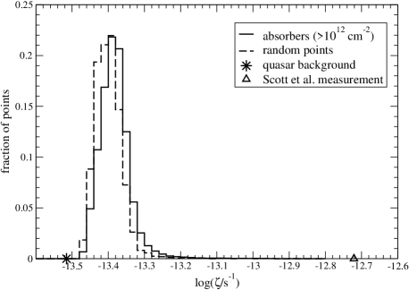
Figure 1: A distribution of values for the direction and frequency averaged ionization rate $\zeta$ is shown for simulated Ly$\alpha$ absorbers with $N_{HI}>10^{12}$ cm^-2 (solid line) and for randomly chosen points within the simulation (dashed line). Also shown (as *) is the assumed minimum background value due to quasars based upon Davé et al. (1999) and Haardt & Madau (1996). The triangle indicates the value for $z<1$ found by Scott et al. (2002) using proximity effect measurements.

A further understanding of the fluctuations in the ionizing background intensity due to galaxies is important for numerous reasons. First of all, the fluctuations need to be understood as a source of uncertainty in measuring the overall background intensity. Histograms of values for the ionization rate $\zeta$ are shown in Fig. 1 for the first simulation, and are shown both for Ly$\alpha$ absorbers ($N_{HI}>10^{12}$ cm^-2) and for random points in the box. The histograms are shown along with the $z=0$ quasar value from Davé et al. (1999), based upon Haardt & Madau (1996) spectra, which is the assumed minimal value for $\zeta$.

Absorbers see higher $\zeta$ values somewhat more often than randomly chosen points, as absorbers arise on average closer to galaxies. Overall the ionization rate seen by Ly$\alpha$ absorbers at $z=0$ varies over about a factor of about two in this simulation. None of the absorbers or random points are exposed to ionization rates which are within about ten percent of the minimal assumed background, although extinction from gas between the absorbers and their ionization sources is not modelled here, so that in reality there may be a few. Most often both the random points and absorbers have $\zeta$ values which are about a factor of 1.4 larger than $\zeta_{b}$. Varying the spectral index of the contribution from these nearby galaxies to $\alpha_{s}\sim 2$ would simply move this peak to $\zeta\sim 1.3\zeta_{b}$. Points with the largest values of $\zeta$ tend to arise at quite low impact parameters from the centres of galaxies, as will be seen in Fig. 4.

Also shown in Fig. 1 is the measurement from Scott et al. (2002) for $z<1$. This measurement has error bars which are large compared to the range of $\zeta$ values shown in this plot, and the lower error bar would be at a slightly higher value than the peak of the plotted histogram, although an extra contribution from star-forming galaxies would move the calculated peak within the measurement error bars. While the galaxies are simulated here at $z\sim 0$, the ionization rate is seen to evolve only by $<0.2$ orders of magnitude between the Scott et al. (2002) measurements at $z<1$ and $z>1$. According to the redshift evolution model they fit, where the background intensity evolves as $(1+z)^{0.017}$, there would be even less difference expected between their measurement for $z<1$ and what would be expected at $z\sim 0$. This could mean that more ionizing radiation escapes from galaxies than is assumed here, although it is more likely that this power law model does not describe the evolution in the ionizing background very well down to $z\sim 0$. However, an additional uniform contribution could also come from galaxies at redshifts $\mathrel{\raise 1.29167pt\hbox{$<$}\mkern-14.0mu\lower 2.58334pt\hbox{$\sim$}}2$, as the universe is optically thin to ionizing photons at these redshifts. Such a contribution would likely be $\sim\zeta_{b}$, as calculated for star-forming galaxies (Giallongo et al. 1997; Shull et al. 1999; Bianchi et al. 2001). Another possible contribution could come from gas in the intragroup medium (Maloney & Bland-Hawthorn 1999; 2001). On the other hand, the other previously mentioned low redshift measurements also tend to be consistent with $\zeta$ values closer to the assumed $\zeta_{b}$, so the value at $z=0$ need not be as large as the Scott et al. (2002) measurement.

While the background intensity detected using the proximity effect is likely to be the most common value in a peaked distribution like the one found here, other values could be seen, for example, when making measurements of the ionization rate around a galaxy in an unusual environment.

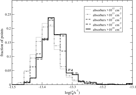
Figure 2: A distribution of values for the ionization rate $\zeta$ is shown for simulated Ly$\alpha$ absorbers with varying limiting neutral column densities. Values of $\zeta$ are binned for absorbers having $N_{HI}>10^{19}$ cm ^-2 (solid line), $>10^{17}$ cm ^-2 (long-dashed line), $>10^{15}$ cm ^-2 (dashed line), $>10^{13}$ cm ^-2 (dot-dashed line), and $>10^{12}$ cm ^-2 (dotted line). Stronger absorbers arise on average closer to luminous galaxies, so that their $\zeta$ values are typically higher.

Table 1: Ionization Rates for Varied Limiting Absorber Column Densities

$N_{HI,min}/cm^{-2}$	$\overline{\log(\zeta/s^{-1})}$	$\sigma$
$10^{12}$	-13.38	0.06
$10^{13}$	-13.38	0.10
$10^{15}$	-13.36	0.33
$10^{17}$	-13.36	0.58
$10^{19}$	-13.36	0.63

For Ly$\alpha$ absorbers with varying limiting neutral column densities, $N_{HI,min}$, the mean values for $\log\zeta$ and standard deviations are shown for the first simulation as also illustrated in Fig. 2. Absorbers with higher $N_{HI}$ appear to have more higher $\zeta$ values in the Figure. Here it can be seen that the mean $\log\zeta$ values change only slightly with limiting $N_{HI}$, but the $\sigma$ values become much larger, indicating more substantial tails of high $\zeta$ values.

Distributions of $\zeta$ values for absorbers are shown in Fig. 2, where the limiting neutral column density for absorbers is varied. It can be seen that more high $\zeta$ values arise for stronger absorbers, as these arise on average closer to galaxies. The average $\log\zeta$ value increases only slightly with limiting $N_{HI}$ however, but the distributions become much less strongly peaked due to larger tails of high $\zeta$ values, as shown in Table 1.

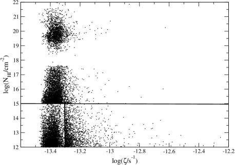
Figure 3: Values of the neutral column density are plotted versus ionization rate for simulated Ly$\alpha$ absorbers. Absorbers are shown as arising from 15,000 lines of sight in the region where $N_{HI}<10^{15}$ cm^-2 and $\zeta>10^{-13.3}$ s^-1, and ten percent of these simulated points are shown in the region where $N_{HI}<10^{15}$ cm^-2 and $\zeta<10^{-13.3}$ s^-1 which would otherwise be further saturated. Absorbers are shown as arising from 60,000 lines of sight through the box where $N_{HI}>10^{15}$ cm^-2. Fairly high values of $\zeta$ can be seen for any value of $N_{HI}$. Few points arise with $N_{HI}\sim 10^{18}$ cm^-2 because absorbers change from neutral to highly ionized at a slightly larger $N_{HI}$ value, as seen in galaxy disc ionization edges.

Values of $\zeta$ are plotted versus neutral column density ($N_{HI}$) for absorbers in Fig. 3. Different numbers of simulated points are plotted in different regions of the plot in order to reduce saturation for low $\zeta$ values and to show more detail for absorbers with high $N_{HI}$. Again the minimum assumed $\zeta=\zeta_{b}$ produces a cutoff on the left side of the plot. Few points are seen with $N_{HI}\sim 10^{18}$ to $10^{19}$, which is related to the galaxy disc ionization edges where $N_{HI}$ falls off quickly with increasing radius around these values. It can be seen that absorbers with a wide range of $N_{HI}$ can be exposed to a wide range of ionization rates. Even more absorbers with a wide range of higher $\zeta$ values would be seen for a wide range of $N_{HI}$ if more ionizing photons were allowed to escape from galaxies in the simulation. This happens even though one might expect absorbers exposed to large $\zeta$ to be ionized away or seen only at lower values of $N_{HI}$. High $N_{HI}$ values with high $\zeta$ still arise, as the galaxies are simulated with a full range of disc inclinations.

Occasionally voids are reported in the Ly$\alpha$ forest (Crotts 1987; Dobrzycki & Bechtold 1991; Cristiani et al. 1995), and there is the possibility that variations in the ionizing background might contribute to such voids. However at this time numbers of voids beyond what would be expected for a random absorber population have not yet been detected for voids smaller than the box size simulated here (Williger 2002).

4 Model Parameter Variations

Table 2: A Summary of the Simulations

Description	$(dN/dz)_{0}$	$(dN/dz)_{0,LL}$	$\overline{\log(\zeta/s^{-1})}$	$\sigma$
1: As in text	25.93	3.91	-13.38	0.06
2: $\tau=2.8$	27.43	4.01	-13.43	0.05
3: $\tau=3.5$	28.85	4.09	-13.47	0.03
4: $\tau=1.5$	21.72	3.69	-13.23	0.10
5: warp$=25^{o}$	24.47	3.69	-13.36	0.07
6: $h_{21}/h_{B}=1.2$	14.06	0.90	-13.44	0.04

The first simulation is as described in the text and illustrated in the Figures. Shown for each simulation in the table are the parameters which were varied (where each simulation is otherwise the same as the first simulation), and the numbers of absorbers $>10^{14.3}$ cm^-2 and Lyman limit absorbers arising per unit redshift in a simulation with 12590 galaxies in a 28.9 Mpc cube, and the mean values for the logarithm of the ionization rate $\zeta$ for Ly$\alpha$ absorbers, and the standard deviation for the distribution of $\log\zeta$.

Several model parameters were varied in further simulations as described in Table 2. The number of Lyman alpha absorbers having $N_{HI}>10^{14.3}$ cm^-2, the number of Lyman limit systems, and the mean and standard deviation $\sigma$ for $\log\zeta$ are shown for each simulation. In each case the mode for the distribution of $\log\zeta$ is very close in value to the mean. In cases where $\sigma$ is relatively large, there tends to be a more substantial tail of points having high $\zeta$ values. The optical depth $\tau$ was varied in order to explore the uncertainty range in the fraction of ionizing photons escaping from galaxies. The value of $\tau=2.8$, preferred for our Galaxy by Bland-Hawthorn (1998), corresponds to a direction-averaged escape fraction of $\sim 2$ percent of the ionizing photons (Bland-Hawthorn & Maloney 2001). In the first simulation, it is assumed that $\tau$ is dependent upon galaxy central surface brightness as discussed above, while in the second simulation we assume $\tau=2.8$ for all galaxies. In the third simulation $\tau=3.5$ is used for all galaxies in order to produce an escape fraction of $\sim 1$ percent, while $\tau=1.5$ is used for all galaxies in the fourth simulation, giving an escape fraction $\sim 10$ percent. A similar distribution for $\zeta$ arises when the value $\tau=2.8$ is assumed for all galaxies as compared to the first simulation. The mean and mode values of $\log\zeta$ correspond to $1.38\zeta_{b}$ in the first simulation, $1.23\zeta_{b}$ in the second simulation, $1.11\zeta_{b}$ where $\tau=3.5$, and $1.95\zeta_{b}$ where $\tau=1.5$. Thus the uncertainty in the fraction of ionizing photons escaping from galaxies means that normal galaxies could contribute between ten percent of the quasar background and an amount about equal to the quasar background.

The typical disc warping angle, which is also rather uncertain, was also varied as shown in the fifth simulation in Table 2. Bland-Hawthorn (1998) has suggested, for example, that there may be a selection bias against detecting highly warped discs in HI because they become more highly ionized by the stars within the galaxy. When the disc warping angle is increased to $25^{o}$ then a slightly higher mean $\log\zeta$ is seen, as more ionizing photons escape higher above the plane of a disc. However the absorbers even in this case are not generally far above the plane of the disc, as the disc is only warped beyond two HI scale lengths.

The distributions in ionization rates seen in the simulations here are generally quite strongly peaked, although there may be more absorbers with high $\zeta$ if there is substantial absorbing gas above the planes of galaxy discs. The contribution to the ionization rate varies by a factor of $45$ for the Bland-Hawthorn (1998) model between polar angles of $0^{o}$ and $80^{o}$ at some distance from a galaxy with $\tau=2.8$. An additional simulation was done where absorbers arise in galaxy haloes with column density profiles obeying equation (24) from Chen et al. (1998). While the absorbing gas is not modeled in this case, the distribution of ionization parameters is found to be similar to that seen in the fifth simulation (where the warping angle $=25^{o}$). Even in this case, however, or for randomly chosen points, or in any case where absorbers arise in random directions relative to galaxies, few of the points or absorbers will arise close to the galactic poles.

The sixth simulation was done with a reduced $h_{21}/h_{B}=1.2$ in order to illustrate a scenario with a more realistic number of Lyman limit absorbers. In this case the mean $\log\zeta$ is slightly lower compared to the first simulation because the simulated absorbers arise typically somewhat closer to the centres of galaxies within the warped outer discs, so that they arise closer to the planes of the discs. In order to make such a scenario realistic, however, an additional population of low column density absorbers would be needed to account for the observed $(dN/dz)_{0}$ as in Bahcall et al. (1996). The additional absorbers could either arise far from luminous galaxies and thus behave more like the random points illustrated in Fig. 1, or they could arise higher above galactic planes where they could be more highly ionized.

A simulation was also run at redshift one by decreasing the box size by a factor of $(1+z)$ and assuming $\zeta_{b}=3.33\times 10^{-13}$ s^-1, again based upon the calculations of Davé et al. (1999) and Haardt & Madau (1996) at $z=1$. Any inconsistency might indicate some galaxy luminosity evolution and/or require more photons to escape from galaxies at $z=1$, although the $\zeta$ distribution was found to be peaked at $3.7\times 10^{-13}$ s^-1, which is between the Scott et al. (2002) measurements for $z<1$ and $z>1$.

5 Relationship to Galaxies

Understanding how the ionizing background varies with galactic environment will be important for understanding what kinds of objects give rise to Ly$\alpha$ absorption, and in which environments Ly$\alpha$ absorption is most likely to arise. Tripp et al. (1998) suggest that no absorption is found near a galaxy cluster due to increased ionization. Fluctuations in the ionizing background may also allow for substantial variations in the environments affecting galaxy formation processes. For example, it has been suggested that dwarf galaxies may form less easily in an intense radiation field (Tully et al. 2002; Efstathiou 1992; Quinn, Katz, & Efstathiou 1996; but see the discussion in Sabatini et al. 2003).

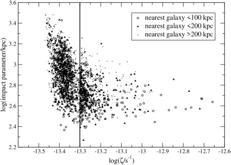
Figure 4: The average impact parameter to the nearest four galaxies having $M_{B}<-16$ is plotted versus ionization rate for simulated Ly$\alpha$ absorbers with $N_{HI}>10^{12}$ cm^-2. Circles indicate points where the nearest galaxy having $M_{B}<-16$ is within 100 kpc, and triangles indicate such a galaxy within 200 kpc. Eight percent of the simulated points with the nearest galaxy $>200$ kpc and fifteen percent of the other points are shown in the region where $\zeta<10^{-13.3}$ s^-1 where the points would otherwise be further saturated. Absorbers with the largest $\zeta$ values tend to be in environments which are rich in nearby galaxies. Absorbers with lower values of $\zeta$ arise at a wide range of averaged impact parameters.

In order to attempt to parametrize the galaxy clustering environment, in Fig. 4 $\zeta$ values are plotted (again for the first simulation) versus the average distance to the nearest four galaxies having $M_{B}<-16$, as observers are generally unable to detect less luminous galaxies around even the nearest absorbers. Again here and in the next two figures, different numbers of simulated points are plotted for $\log\zeta<-13.3$ values in order to reduce the saturation in the plot. The nearest four galaxies are used because the ionizing background is likely to be somewhat higher even in a group environment in addition to being higher in a rich cluster. The shapes of the plotted points give more information about the nearest single galaxy with $M_{B}<-16$. The $\zeta$ values are shown for absorbers with $N_{HI}>10^{12}$ cm^-2. Most of the points with $\zeta\sim\zeta_{b}$ are far from luminous galaxies, while those with higher $\zeta$ arise more often closer to luminous galaxies. However, selection effects against LSB galaxies may make this correlation less clearly visible to an observer. Some higher $\zeta$ values can arise even far from luminous galaxies, however, as it was assumed that some ionizing radiation escapes even from dwarf galaxies which are not assumed to be strongly clustered. Still the presence of any luminous galaxy may have a more important effect on the ionization rate rather than the overall clustering environment, as large $\zeta$ values tend to arise more often when a luminous galaxy is within 200 kpc.

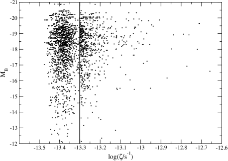
Figure 5: Absolute magnitudes are plotted for galaxies where Ly$\alpha$ absorption ($>10^{12}$ cm^-2) is known to arise in the simulation versus ionization rate for the absorber. Ten percent of the simulated points are shown for $\log\zeta<-13.3$ where the figure would otherwise be further saturated. Horizontal lines are seen because numerous absorbers can arise close to a particular simulated luminous galaxy. More high $\zeta$ absorbers are seen around luminous galaxies simply because these galaxies are assumed to have more absorbing gas around them so that more absorbers with any $\zeta$ value arise. Fairly high values of $\zeta$ can arise around galaxies with any $M_{B}$ value.

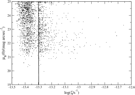
Figure 6: Central surface brightnesses are plotted for galaxies where Ly$\alpha$ absorption ($>10^{12}$ cm^-2) arises nearby versus ionization rate for the absorber. Ten percent of the simulated points are shown for $\log\zeta<-13.3$ where the figure would otherwise be further saturated. High $\zeta$ values can arise around galaxies with a wide range of central surface brightness values.

In Figs. 5 and 6, $\zeta$ values are plotted versus galaxy luminosity and central surface brightness for each absorber, where their associated galaxies are known from the simulation. (Note that an observer might identify a different galaxy as associated with an absorber, as discussed in Linder (2000).) Points are seen to lie on horizontal lines in either plot, as galaxies which are luminous or moderately low in surface brightness are assumed to have large absorption cross sections for their surrounding gas and give rise to numerous absorbers within the simulation. It can be seen in either plot that absorbers arising around galaxies with a wide range of properties are exposed to a wide range of ionization rates. Thus variations in $\zeta$ happen around particular galaxies, although these galaxies can have a wide range of properties. High $\zeta$ values will be seen most often in locations where absorbers arise most often, such as those close to luminous galaxies. Yet many more faint galaxies exist, where some absorbers with high $\zeta$ values can also be seen, and no evidence is seen for a variation in the average $\zeta$ values with galaxy luminosity or surface brightness.

The ionization rate tends to be higher close to galaxies and in regions of higher galaxy density where Ly$\alpha$ absorbers often arise, but how much is the intergalactic medium affected on average by ionizing radiation from galaxies? The lowest $\zeta$ values tend to be seen when looking as far as possible from a luminous galaxy, as can be seen in Fig. 7. A fall-off can be seen in the average $\zeta$ value with impact parameter from a galaxy with $M_{B}<-16$, and such a fall-off appears to be steeper for more luminous galaxies. Again this plot may be affected by luminous galaxies having more absorbers with high $\zeta$ values around them simply because more absorbing gas is assumed to be located around luminous galaxies.

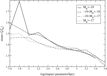
Figure 7: The average ionization rate, shown in units of the assumed quasar background $\zeta_{b}$, is shown here for absorbers $>10^{12}$ cm^-2 versus impact parameter to the nearest galaxy with $M_{B}>-16$. A solid line is shown where the nearest such galaxy has $M_{B}<-19$, a dashed line for $-19<M_{B}<-18$, dot-dashed for $-18<M_{B}<-17$, and dotted for $M_{B}<-17$. It can be seen that the average $\zeta$ value for absorbers decreases with increasing impact parameter from a luminous galaxy, and the decrease appears to be steepest for the most luminous galaxies. Note that the error bars based upon the standard deviation in simulated $\zeta$ values would be smallest for impact parameter values in the centre of the plot where $\zeta/\zeta_{b}\sim 1.4$, as there are fewer data points for high and low $\zeta$ values.

A less biased view of the ionization of the intergalactic medium can be seen from looking at a similar plot of the average $\zeta$ value versus impact parameter to the nearest galaxy for random points rather than absorbers, as shown in Fig. 8. While it becomes even more difficult here to simulate points which are very close to galaxies, it can be seen even more clearly that the intergalactic medium is more highly ionized at points which are closer to more luminous galaxies. While Fig. 7 is a prediction of what observers might see if they are able to measure $\zeta$ for numerous absorbers, Fig. 8 is a better representation of how the ionization of the intergalactic medium could be simulated.

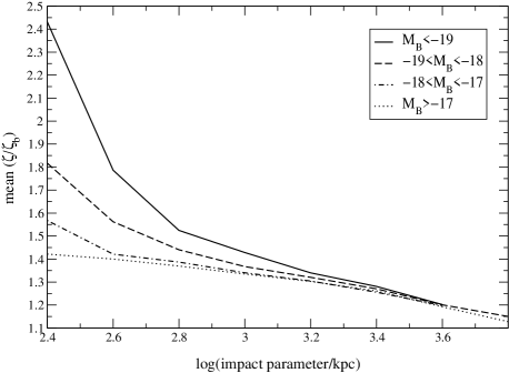
Figure 8: The average ionization rate, shown in units of the assumed quasar background $\zeta_{b}$, is shown here at randomly chosen points versus impact parameter to the nearest galaxy with $M_{B}>-16$. A solid line is shown where the nearest such galaxy has $M_{B}<-19$, a dashed line for $-19<M_{B}<-18$, dot-dashed for $-18<M_{B}<-17$, and dotted for $M_{B}<-17$. Compared to the previous figure, it can be seen even more clearly here that the average $\zeta$ value for absorbers decreases with increasing impact parameter from a luminous galaxy, and the decrease is the steepest for the most luminous galaxies.

6 Conclusions

Normal galaxies are likely to contribute at least thirty to forty percent of what quasars do to the ionizing background of Lyman continuum photons at zero redshift, assuming that ionizing photons escape from other galaxies in an analogous manner to the Bland-Hawthorn (1998) model of our Galaxy where $\sim 2$ percent of ionizing photons escape. Allowing for some uncertainty in this direction-averaged ionizing photon escape fraction, assuming that between $\sim 1$ and $\sim 10$ percent of ionizing photons escape means that the contribution to the ionizing background from normal galaxies could be between $\sim 10$ and $\sim 100$ percent of the assumed quasar contribution. This ultraviolet background is important for ionizing gas surrounding galaxies and within the intergalactic medium. This gas gives rise to Ly$\alpha$ absorption and makes an uncertain contribution to the baryon content in the local universe due to uncertainties in ionization intensities and mechanisms.

Distant quasars at somewhat higher redshifts will ionize the low redshift universe in a relatively uniform manner, but ionizing radiation escaping from normal galaxies at low redshift will result in local fluctuations in the ionizing background. Fluctuations have been found in the ionization rate of gas around simulated galaxies, which will give rise to variations in the neutral gas fractions in Ly$\alpha$ absorbers with a wide range of neutral column densities. A wide range of ionization rates are found to arise close to galaxies having a wide range of properties, but normal galaxies also play an important role in ionizing the more distant intergalactic medium. Ionization rates for absorbers are found to be about twice as high as the quasar background on average when looking at $\sim 200$ kpc from a luminous galaxy, about 1.4 times the quasar background when looking at $\sim 1$ to 2 Mpc from a luminous galaxy, and only as little as $\sim 1.1$ times the quasar background when looking as far as possible from luminous galaxies. Luminous star forming galaxies, which may contain rather clumpy dust and thus have more complex extinction behaviour than was modelled here, will also give rise to both local and larger scale fluctuations in the ionizing background.

Fluctuations in the ionizing background may have implications for the formation and evolution, and our ability to detect, smaller objects located near luminous galaxies, such as dwarf galaxies and high velocity clouds. Such fluctuations will also give rise to variations in galaxy disc ionization edges, which will have implications for the column density distribution of Lyman limit absorbers. Fluctuations in the ionizing background may also have some implications for the nature of Ly$\alpha$ absorbers and their relationship to galaxies. If galaxies play an important role in ionizing the gas around them, gas which must make some contribution to Ly$\alpha$ absorption, then further constraints may be made on models for galaxies giving rise to absorption. Gas which is too close to a luminous galaxy, and in particular that located far above the plane of the disc, will be exposed to more ionizing radiation than absorbing gas which is ionized largely by a quasar background, possibly reducing the number density of absorbers that will arise in such environments. Variations in the fractions of ionizing radiation that escape from galaxies with various properties may be important for determining what kinds of galaxies can give rise to absorption. A further understanding of the distribution of ionization rates will enable us to learn more about chemical abundances using metal absorption line systems.

The fluctuations in the ionizing background are not seen to be substantial in the simulations here however, although most absorbers are assumed to arise fairly close to the planes of galaxy discs. Larger variations in the photoionization rates would only be seen if substantial amounts of absorbing gas are concentrated above galactic poles, although in this case the gas might include components which are ejected from the galaxies so that collisional ionization processes might also be important.

Appendix A Relationship between the Column Density Profile in a Disc and the Column Density Distribution

Suppose absorbers arise in the outer parts of galaxy discs, where the column density $N_{HI}$ in each disc falls off with radius $r$ as a power law where $N_{HI}\propto r^{-p}$. The neutral column density distribution $d{\cal{N}}/dN_{HI}$ resulting from these absorbers in then $d{\cal{N}}/dN_{HI}=d{\cal{N}}/dr\times dr/dN_{HI}=2\pi r\times dr/dN_{HI}$. Since $dN_{HI}/dr\propto r^{-(p+1)}$ from the assumed column density profile then $d{\cal{N}}/dN_{HI}\propto r^{(p+2)}\propto(N_{HI}^{-1/p})^{(p+2)}$. Thus when the neutral column density distribution in each outer disc falls off as a power law with exponent $-p$, then the resulting neutral column density distribution is also a power law having exponent $-\epsilon$, where $d{\cal{N}}/dN_{HI}\propto N_{HI}^{-\epsilon}\propto N_{HI}^{-(p+2)/p}$ and $p=2/(\epsilon-1)$.

Appendix B Polar Angle Calculation

At a point $(x,y,z)$ in space where the ionization rate is calculated, each galaxy $i$ contributes emission which is seen at angle $\Theta_{i}\ (\leq\pi/2)$ from the galaxy’s pole. Each galaxy has a randomly simulated inclination $\theta$ between the disc plane and the $z$-axis, thus chosen from a uniform distribution in $\cos\theta$, and a random orientation $\phi$, where $0\leq\phi<2\pi$.

The angle between the galaxy’s rotation axis given by the vector ${\bf v}$ and the line given by the vector ${\bf d}=(x-x_{i},y-y_{i},z-z_{i})$ equals

$$\min(\angle({\bf v},{\bf d}),\angle(-{\bf v},{\bf d}))$$

$$= \min\left(\cos^{-1}\left(\frac{\langle{\bf v},{\bf d}\rangle}{||{\bf v}||\cdot||{\bf d}||}\right),\cos^{-1}\left(\frac{\langle{\bf v},-{\bf d}\rangle}{||{\bf v}||\cdot||{\bf d}||}\right)\right)$$

$$= \cos^{-1}\left(\frac{|\langle{\bf v},{\bf d}\rangle|}{||{\bf v}||\cdot||{\bf d}||}\right)$$

$$= \cos^{-1}\left(\frac{|v_{x}d_{x}+v_{y}d_{y}+v_{z}d_{z}|}{||{\bf v}||\cdot||{\bf d}||}\right).$$

This angle is always in the interval $[0,\pi/2].$ Here $||{\bf d}||=\sqrt{d_{x}^{2}+d_{y}^{2}+d_{z}^{2}}$. The vector ${\bf v}$ is produced by rotating the vector $(0,0,1)$ first by $\pi/2-\theta$ in the $xz$-plane, which gives the vector $(\cos\theta,0,\sin\theta)$, and then rotating by angle $\phi$ in the $xy$-plane, which gives the vector $(\cos\theta\cos\phi,-\cos\theta\sin\phi,\sin\phi).$ Hence $||{\bf v}||=1$.

The polar angle is thus

$$\Theta_{i}=\cos^{-1}\left(\frac{|d_{x}\cos\theta\cos\phi-d_{y}\cos\theta\sin\phi+d_{z}\sin\theta|}{(d_{x}^{2}+d_{y}^{2}+d_{z}^{2})^{1/2}}\right)$$ (5)

where

$$d_{x}=x-x_{i}$$ (6)

$$d_{y}=y-y_{i}$$ (7)

$$d_{z}=z-z_{i}$$ (8)

for galaxy $i$ centred at $(x_{i},y_{i},z_{i})$.

References

- (1) Bahcall, J. N. et al. 1996, ApJ, 457, 19
- (2) Bergeron, J., & Boissé, P. 1991, A&A, 243, 344
- (3) Bianchi, S., Cristiani, S., & Kim, T.-S. 2001, A&A, 376, 1
- (4) Bland-Hawthorn, J., Taylor, K., Veilleux, S. & Shopbell, P. L. 1994, ApJ, 437, L95
- (5) Bland-Hawthorn, J., 1998, in D. Zaritsky, ed., Galaxy Halos, ASP Conf. Ser. 136, San Francisco, p. 113
- (6) Bland-Hawthorn, J., Freeman, K. C., & Quinn, P. J. 1997, ApJ, 490, 143
- (7) Bland-Hawthorn, J. & Maloney, P. 1999, ApJ, 510, L33
- (8) Bland-Hawthorn, J. & Maloney, P. 2001, ApJ, 550, L231
- (9) Bochkarev, N. G. & Sunyaev, R. A., 1977, Soviet Astr., 21, 542
- (10) Bowen, D. V., Blades, J. C., & Pettini, M. 1996, ApJ, 464, 141
- (11) Bowen, D. V. Tripp, T. M., & Jenkins, E. B., 2001, AJ, 121, 1456
- (12) Bowen, D. V., Pettini, M., & Blades, J. C. 2002, ApJ, 580, 169
- (13) Briggs, F. H. 1990, ApJ, 352, 15
- (14) Cayatte, V., Kotanyl, C., Balkowski, C., & Van Gorkom, J. H. 1994, AJ, 107, 1003
- (15) Charlton, J. C., Salpeter, E. E., & Hogan, C. J. 1993, ApJ, 402, 493
- (16) Charlton, J. C., Salpeter, E. E., & Linder, S. M. 1994, ApJ, 430, L29
- (17) Chen, H.-W., Lanzetta, K. M., Webb, J. K., Barcons, X. 1998, ApJ, 498, 77
- (18) Chen, H.-W., Lanzetta, K. M., Webb, J. K., Barcons, X. 2001, ApJ, 560, 101
- (19) Cohen, J. G., 2001, AJ, 121, 1275
- (20) Corbelli, E. & Salpeter, E. E. 1993, ApJ, 419, 104
- (21) Cristiani S., D’Odorico S., Fontana A., Giallongo E., & Savaglio S. 1995, MNRAS 273, 1016
- (22) Crotts A. P. S. 1987, MNRAS, 228, 41
- (23) Davé, R., Hernquist, L., Katz, N., & Weinberg, D. H. 1999, ApJ, 511, 521
- (24) Deharveng, J.-M., Faïsse, S., Milliard, B., & Le Brun, V. 1997, A&A, 325, 1259
- (25) Dobrzycki A. & Bechtold J. 1991. ApJ, 377, L69
- (26) Donahue, M., Aldering, G., & Stocke, J. T., 1995, ApJ, 450, L45
- (27) Dove, J. B. & Shull, J. M. 1994a, ApJ, 423, 196
- (28) Dove, J. B. & Shull, J. M. 1994b, ApJ, 430, 222
- (29) Dove, J. B., Shull, J. M., & Ferrara, A. 2000, ApJ, 531, 846
- (30) Efstathiou, G. 1992, MNRAS, 256, 43
- (31) Fardal, M. A., Giroux, M. L., & Shull, J. M. 1998, AJ 115, 2206
- (32) Giallongo, E., Fontana, A., & Madau, P. 1997, MNRAS, 289, 629
- (33) Goldader, J. D., Meurer, G. Heckman, T. M., Seibert, M., Sanders, D. B., Calzetti, D., & Steidel, C. C. 2000, ApJ, 568, 651
- (34) Haardt, F. & Madau, P. 1996, ApJ, 461, 20
- (35) Henry, R. C. 2002, ApJ, 570, 697
- (36) Hoffman, G. L., Lu, N. Y., Salpeter, E. E., Farhat, B., Lamphier, B., & Roos, T. 1993, AJ, 106, 39
- (37) Hurwitz, M., Jelinsky, P., & Van Dyke Dixon, W., 1997, ApJ, 378, 131
- (38) Kulkarni, V. P., & Fall, S. M. 1993, ApJ, 413, L63
- (39) Lanzetta, K. M., Bowen, D. V., Tytler, D., & Webb, J. K. 1995a, ApJ, 442, 538
- (40) Lanzetta, K. M., Wolfe, A. M., & Turnshek, D. A. 1995b, ApJ, 440, 435
- (41) Le Brun, V., Bergeron, J., & Boissé, P. 1996, A&A, 306, L691
- (42) Leitherer, C., Ferguson, H. C., Heckman, T. M., & Lowenthal, J. D. 1995, ApJ, 454, L19
- (43) Linder, S. M. 1998, ApJ, 495, 637
- (44) Linder, S. M. 2000, ApJ, 529, 644
- (45) Maloney, P. 1993, ApJ, 414, 41
- (46) Maloney, P. R. & Bland-Hawthorn, J. 1999, ApJ, 522, L81
- (47) Maloney, P. R. & Bland-Hawthorn, J. 2001, ApJ, 553, L129
- (48) McGaugh, S. S. 1996, MNRAS, 280, 337 M. A., 1999, AJ, 118, 1450
- (49) McLin, K. M., Giroux, M. L., & Stocke, J. T., 1998, in D. Zaritsky, ed., Galaxy Halos, ASP Conf. Ser. 136, San Francisco, p. 175
- (50) O’Neil, K., Bothun, G. D., & Impey, C. D. 1997, BAAS, 29, 1398
- (51) Penton, S. V., Stocke, J. T., & Shull, J. M. 2002, ApJ, 565, 720
- (52) Quinn, T., Katz, N., & Efstathiou, G. 1996, MNRAS, 278, L49
- (53) Sabatini, S., Davies, J. I., Scaramella, R., Smith, R., Baes, M., Linder, S. M., Roberts, S. 2003, & Testa, V., MNRAS, in press
- (54) Scott, J., Bechtold, J., Morita, M., Dobrzycki, A., & Kulkarni, V. 2002, ApJ, 571, 665
- (55) Shull, J. M., Stocke, J. T., & Penton S. 1996, AJ, 111, 72
- (56) Shull, J. M., Roberts, D., Giroux, M. L., Penton, S. V., & Fardal, M. A. 1999, AJ, 118, 1450
- (57) Soneira, R. M. & Peebles, P. J. E. 1978, AJ, 83, 845
- (58) Steidel, C. C., 1995, in G. Meylan, ed., QSO Absorption Lines, Springer–Verlag, Berlin, p. 139
- (59) Steidel, C. C., Dickinson, M., Meyer, D. M., Adelberger, K. L., & Sembach, K. R. 1997, ApJ, 480, 568
- (60) Stengler-Larrea, E. A., et al. 1995, ApJ, 444, 64
- (61) Stocke, J. T., Case, J., Donahue, M., Shull, J. M., & Snow, T. P. 1991, ApJ, 374, 72
- (62) Stocke, J. T., Shull, J. M., Penton, S., Donahue, M., & Carilli, C. 1995, ApJ, 451, 24
- (63) Storrie-Lombardi, L. J., McMahon, R. G., Irwin, M. J., & Hazard, C. 1994, ApJ, 427, L13
- (64) Sutherland, R., & Shull J. M. 1999, as referenced in Shull et al. (1999)
- (65) Tripp, T. M., Lu, L., & Savage, B. D. 1998, ApJ, 508, 200
- (66) Tufte, S. L., Reynolds, R. J., & Haffner, L. M. 1998, ApJ, 504, 773
- (67) Tully, R. B., Somerville, R. S., Trentham, N., & Verheijen, M. A. W., 2002, ApJ, 569, 573
- (68) Tumlinson, J., Giroux, M. L., Shull, J. M., & Stocke, J. T. 1999, AJ, 118,2148
- (69) Turnshek, D. A., Rao, S., Nestor, D., Lane, W., Monier, E., Bergeron, J., Smette, A. 2000, ApJ, 553, 288
- (70) Vacca, W. D., Garmany, C. D., & Shull, J. M. 1996, ApJ, 460, 914
- (71) Vogel, S. N., Weymann, R., Rauch, M. & Hamilton, T. 1995, ApJ, 441, 162
- (72) Vogel, S. N., Weymann, R. J., Veilleux, S., & Epps, H. W. 2002, in J. S. Mulchaey & J. T. Stocke, eds.,Extragalactic Gas at Low Redshift, ASP Conf. Ser. 254, San Fransisco, p. 363
- (73) Williger, G. 2002 in ’The IGM/Galaxy Connection’, Kluwer, in press