Quantum corrections to microscopic diffusion constants

We review the state of the art regarding the computation of the resistance coefficients in conditions typical of the stellar plasma, and compare the various results studying their effect on the solar model. We introduce and discuss for the first time in an astrophysical context the effect of quantum corrections to the evaluation of the resistance coefficients, and provide simple yet accurate fitting formulae for their computation. Although the inclusion of quantum corrections only weakly modifies the solar model, their effect is growing with density, and thus might be of relevance in case of denser objects like, e.g., white dwarfs.

1 Introduction

Basic physical considerations suggest that, in addition to convective mixing – routinely included in stellar evolution computations – additional transport processes are efficient within the stellar interior; they are driven by pressure, temperature and chemical abundance gradients, and by the effect of radiative pressure on the individual ions. These processes are collectively called ’diffusion processes’, and their inclusion in stellar evolution computations is necessary in order to satisfy the helioseismological constraint for the solar models (Bahcall et al. 1995).

In general, individual ions are forced to move under the influence of pressure as well as temperature gradients, which both tend to move the heavier elements toward the centre of the star, and of concentration gradients that oppose the above processes. Radiation, which causes negligible diffusion in the Sun, pushes the ions toward the surface, whenever the radiative acceleration of an individual ion species is larger than the gravitational acceleration. The speed of the diffusive flow depends on the collisions with the surrounding particles, as they share the acquired momentum in a random way. It is the extent of these ’collision’ effects that dictates the timescale of element diffusion within the stellar structure, once the physical and chemical profiles are specified. The most general treatment for the element transport in a multicomponent fluid associated with diffusion is provided by Burgers’ (1969, B69) equations. In these equations the effect of collisions between ions is represented by the so-called resistance coefficients, i.e. the matrices $K$, $z$, $z^{\prime}$, $z^{\prime\prime}$, whose precise evaluation is fundamental in order to estimate correctly the diffusion timescales for the various elements.

Recent spectroscopic determinations of Fe and Li abundances in Galactic globular cluster turn-off stars discussed in, e.g., Gratton et al. (2001) or Bonifacio et al. (2002), have shown that the present standard treatment of diffusion is in disagreement with the observed surface abundance of these two elements in stars of globular clusters (for the Li problem see, e.g., Michaud et al. 1984 or Vauclair & Charbonnel 1995). In the light of these results, it is very important to conclusively assess how much of this discrepancy is due to an incorrect treatment of the diffusion process, and how much is due to competing rotationally induced or other non-standard macroscopic mixing phenomena, which inhibit the efficiency of diffusion.

In this paper the state of the art regarding the computation of the resistance coefficients in conditions typical of the stellar plasma is reviewed and a detailed comparison of the results from different authors is performed. The effect of different resistance coefficients on solar models is examined, too. Moreover, we introduce and discuss for the first time in astrophysical computations the effect of quantum corrections to the evaluation of the resistance coefficients. We also provide simple fitting formulae for accurate calculations of resistance coefficients including the appropriate quantum corrections. In § 2 we compare existing determinations of the resistance coefficients, and discuss the differences on solar models; in § 3 we determine the appropriate quantum corrections to these coefficients, and conclusions will follow in § 4. Analytical formulae for the computations of updated resistance coefficients, including quantum corrections, are given in the appendices.

2 Classical treatment of element diffusion

The diffusion of elements in a multicomponent fluid can be treated either according to the Chapman & Cowling (1970) or the B69 formalism. We are following the latter description, which is equivalent to the so-called “second approximation” in Chapman & Cowling (1970). It would be desirable to use a higher order approximation, because an uncertainty of the order of 10% is introduced by using only the second one (Roussel-Dupré 1982), independent of the accuracy in the resistance coefficients. But this can only be done in the scheme of Chapman & Cowling (1970), which becomes very cumbersome for gases with more than two components.

2.1 Existing calculations of resistance coefficients

Burgers’ equations are obtained assuming the gas particles have approximate Maxwellian velocity distributions; the temperatures are the same for all particle species; the mean thermal velocities are much larger than the diffusion velocities; magnetic fields are unimportant. Burgers’ scheme involves the resistance coefficients $K$, $z$, $z^{\prime}$ and $z^{\prime\prime}$; following Mason et al. (1967, MMS67), they can be expressed in terms of the so-called reduced collision integrals ${\Omega^{(l,s)}_{ij}}^{\ast}$ (Hirschfelder et al. 1954), according to the following relationships:

$$\frac{K_{ij}}{K_{ij}^{0}} = 4\frac{{T^{\ast}_{ij}}^{2}\,{\Omega^{(1,1)}_{ij}}^{\ast}}{\ln\left(\Lambda_{ij}^{2}+1\right)}\mathrm{,}$$ (1)

$$z_{ij} = 1-1.2\frac{{\Omega^{(1,2)}_{ij}}^{\ast}}{{\Omega^{(1,1)}_{ij}}^{\ast}}\mathrm{,}$$ (2)

$$z_{ij}^{\prime} = 2.5-\frac{6\,{\Omega^{(1,2)}_{ij}}^{\ast}-4.8\,{\Omega^{(1,3)}_{ij}}^{\ast}}{{\Omega^{(1,1)}_{ij}}^{\ast}}\mbox{\quad and}$$ (3)

$$z_{ij}^{\prime\prime} = 2\frac{{\Omega^{(2,2)}_{ij}}^{\ast}}{{\Omega^{(1,1)}_{ij}}^{\ast}}\mathrm{,}$$ (4)

where

$$T^{\ast}_{ij} = k_{\mathrm{B}}T\frac{\lambda_{\mathrm{D}}}{\left|Z_{i}Z_{j}e^{2}\right|}\quad\mbox{and}$$ (5)

$$K_{ij}^{0} = \frac{2}{3}\sqrt{\frac{2\mu_{ij}\pi}{(k_{\mathrm{B}}T)^{3}}}\left(Z_{i}Z_{j}e^{2}\right)^{2}n_{i}n_{j}\ln\left(\Lambda_{ij}^{2}+1\right)$$ (6)

with $\lambda_{\mathrm{D}}=\sqrt{k_{\mathrm{B}}T/(4\pi n_{\mathrm{e}}e^{2})}$ being the Debye-length, $\Lambda_{ij}=4T_{ij}^{\ast}$ the plasma parameter, $\mu_{ij}=m_{i}m_{j}/(m_{i}+m_{j})$ the reduced mass, and $Z_{i}$, $m_{i}$ and $n_{i}$ the charge number, mass and particle number density of species $i$, respectively. The collisions between the particles of the stellar plasma determine the values of the ${\Omega^{(l,s)}_{ij}}^{\ast}$ integrals; the physics of the collisions is specified by some form of the Coulomb interaction which, as a first approximation, can be described by a pure Coulomb potential with a long-range cut-off distance, usually assumed to be $\lambda_{\mathrm{D}}$. According to B69, using this truncated pure Coulomb potential the resistance coefficients become

$$\frac{K_{ij}}{K_{ij}^{0}} = 2\,\frac{\ln\Lambda_{ij}-C_{\mathrm{E}}\pm\frac{\pi^{2}}{4}}{\ln\left(\Lambda_{ij}^{2}+1\right)}{\rm,}$$ (7)

$$z_{ij} = 0.6{\rm,}$$ (8)

$$z^{\prime}_{ij} = 1.3\mbox{\quad and}$$ (9)

$$z^{\prime\prime}_{ij} \approx 2\mathrm{,}$$ (10)

where $C_{\mathrm{E}}$ is Euler’s constant and the alternative signs in Eq. (7) represent repulsive ($+$) and attractive ($-$) particles, respectively. For high densities and thus small values of the plasma parameter, the resistance coefficients become negative (for an attractive potential already for $\Lambda\lesssim 20$). Since in stellar plasmas, in particular in case of white dwarfs, $\Lambda$ is often much smaller than this value, more elaborate computations have been performed.

Table 1: Quantities in this work, which follows basically MMS67, and their relation to quantities used by other authors.

This work	M84	IM85	P86
$\Lambda_{ij}$	$\Lambda_{ij}$	$x_{ij}$	$\gamma_{ij}$
${T_{ij}^{\ast}}^{2}{\Omega^{(s,t)}_{ij}}^{\ast}$	—	—	$\frac{1}{4}F_{ij}^{(st)}$
$\Phi_{ij}$	$\Phi$	$\Phi$	$\Psi_{ij}$
$K^{0}_{ij}$	$(K_{ij})_{0}$	$K^{0}_{ij}$	$\epsilon_{ij}\times\frac{16}{3}x_{i}x_{j}nmM_{i}M_{j}\mathrm{e}^{\Psi_{ij}}$

More accurate collision integrals have been obtained by considering a Debye-Hückel type of potential

$$V_{ij}(r)=\frac{Z_{i}Z_{j}e^{2}}{r}\;\mathrm{e}^{-r/\lambda_{\mathrm{D}}}$$ (11)

where $r$ is the particle distance. The results are provided either in tabulated form by MMS67 or as fitting formulae by Muchmore (1984, M84), Iben & MacDonald (1985, IM85) and Paquette et al. (1986, P86). In the latter cases the integrals are given as functions of

$$\Phi_{ij}=\ln\left(\ln(1+\Lambda_{ij}^{2})\right).$$ (12)

Different notations for the same physical quantities have been used by these groups; in Table 1 their relations to the present work are summarized. M84, IM85 and P86 argue that while $\lambda_{\mathrm{D}}$ is an appropriate screening distance at low densities, the Debye sphere loses its significance at high densities, in which case a more appropriate screening distance is the mean interionic distance; thus they suggest to use in the actual stellar model computations the larger of $\lambda_{\mathrm{D}}$ or the mean interionic distance. Whatever one chooses for the actual screening distance, its value has to be employed as $\lambda_{\mathrm{D}}$ in Eq. (5) to obtain the appropriate value for $\Lambda_{ij}$ for determining the collision integrals. We also remark that, at least for the entire evolution of the Sun up to now, $\lambda_{\mathrm{D}}$ has always been larger than the mean interionic distance.

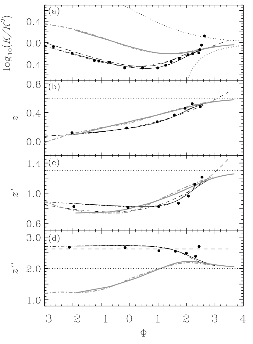
Figure 1: The resistance coefficient $K$ (a), $z$ (b), $z^{\prime}$ (c) and $z^{\prime\prime}$ (d) as computed by B69 (dotted), MMS67 (solid), M84 (short-dashed), P86 (dash-dotted) and IM85 (long-dashed line). The dark black lines indicate the case of repulsive potentials, while the brighter ones show the values for attractive forces (not computed by M84 and IM85). The dots represent the actual values computed by M84.

The results of the different groups are compared in Fig. 1. Noticeably, given that they use all the same physical assumptions, they all got very similar values, but they all differ significantly from Burgers’ results at higher densities (i.e., lower values of $\Phi$), where his approximations are not adequate anymore. M84’s formulae for the case of a repulsive potential have been obtained by fitting solely the values represented by dots in Fig. 1. Although the formulae work pretty well overall, $z^{\prime\prime}$ deviates considerably at $\Phi=2$ from the mean value of $2.6$, and the almost linear behaviour of $z^{\prime}$ for $-3<\Phi<1$ is only poorly reproduced.

Figure 2: The relative difference of $K$ (a), $z$ (b), $z^{\prime}$ (c) and $z^{\prime\prime}$ (d) between our analytic fits and the values calculated by P86. The solid line represents the case of a repulsive potential, the short-dashed one the case of an attractive potential; the dotted line indicates the line of zero difference. Also shown in (a) is the difference between the IM85’s and P86’s results (long-dashed) and IM85’s and M84’s results (dash-dot-dot-dotted line).

The supposedly most accurate calculation of the collision integrals has been performed in P86, where cubic splines for 50 equally spaced intervals in $\Phi$ are provided; the results agree very well with the tabulation by MMS67. To obtain more manageable but still accurate formulae, we fitted polynomials of at most 5^th order to their values for $-2.5<\Phi<3$; this enables to compute diffusion of elements up to Fe in stars on the main sequence and to follow with sufficient accuracy the early white dwarf cooling phase. The numerical values for the polynomial coefficients are given in Appendix A.

In Fig. 2 the relative differences between our fitting formulae and the values of P86 are shown. For the case of a repulsive potential ($e$-$e$ or ion-ion collisions) the results of P86 for all quantities can be reproduced with an accuracy better than 2%; for an attractive potential ($e$-ion collisions) the accuracy is still well within 5%, and for a large range of $\Phi$ values it is certainly better than 3%. Taking into account that the results of different groups for the same physical assumptions, e.g., between IM85 and P86 (long-dashed line in Fig. 2a), differ by up to 15%, we consider our polynomial fits to be sufficiently accurate.

In main sequence stars the value of $\Phi$ does not deviate considerably from $2$ for H and He (see Fig. 3b), thus constant values for $z$, $z^{\prime}$ and $z^{\prime\prime}$ are usually assumed. Moreover, in stellar plasmas the amount of element diffusion is basically determined by ion-ion collisions, and as the differences for attractive and repulsive potential are small when $\Phi\sim 2$, the resistance coefficients for a repulsive potential are often employed for all cases. For instance, the widely used diffusion routine by (Thoul et al. 1994, TBL) uses the values of B69 for $z$, $z^{\prime}$ and $z^{\prime\prime}$ (Eq. 8–10) while for $K$ the fitting formula of IM85 has been implemented. This assumption overestimates $z$ and $z^{\prime}$, but underestimates $z^{\prime\prime}$, which results in a somewhat too high efficiency of the thermal diffusion (see M84).

2.2 Effect on solar models

Figure 3: a) The relative difference between the seismic model of Basu et al. (1997) and solar models computed with different resistance coefficients: S1 (solid line), S2 (dotted), S3 (dash-dot-dot-dotted), S4 (short-dashed), S5 (long-dashed) and S6 (dash-dotted). The resistance coefficients used in the models are summarized in Table 2. b) The run of $\Phi$ for H⁺-H⁺ (solid) and He²⁺-He²⁺ collisions (dashed line) in solar models.

In order to estimate the influence of different choices of the resistance coefficients on the solar structure, we computed various solar models utilizing the stellar evolution code and element diffusion routine described in Schlattl (2002) and references therein. Element diffusion is treated following the scheme by TBL, considering in addition the effect of electron degeneracy and partial ionization of elements; the latter is implemented by defining a mean charged ion per element, instead of computing diffusion for each ion separately. This treatment of partial ionization is sufficient for a large range of stellar masses, including the Sun. We neglect radiative levitation, which leads to a tiny improvement of the theoretical sound-speed profile compared to the Sun of at most 0.025% at $r\approx 0.6\,R_{\odot}$ (see Turcotte et al. 1998).

The sound speeds of various solar models computed using different choices of the collision integrals are summarized in Fig. 3a, while the variation of He and metal abundances at the surface and at the centre of the Sun are shown in Fig. 4. The solid line represents a solar model (S1, see Table 2) computed with $K$ of IM85 and constant values for the $z$’s of B69  corresponding to the values used by TBL. This description has been used, for instance, in solar models of Bahcall et al. (1998) and Schlattl (2002). Dropping the assumption of constant $z$’s, and using instead the functions of M84, the sound-speed difference to a seismic model becomes about 4 times higher for $0.3<r/R_{\odot}<0.65$ (dotted line in Fig. 3a; S2), caused by the reduced thermal diffusion efficiency. The latter leads also to a diminished surface depletion of He and metals (see Fig. 4). When one employs, in addition, M84’s values for $K$ instead of the IM85 ones, the difference to model S1 (dash-dot-dot-dotted line) lowers, because M84 computed an about 7% smaller value for $K$ than IM85 (Fig. 1a) for the relevant $\Phi$ range, which results in slightly higher diffusion velocities.

Figure 4: a) The surface depletion of various elements in solar models with different collision integrals from the pre-main sequence until now. The line-styles correspond to Fig. 3. On the right hand side the change in the overall metallicity is shown. b) Like a), but for the centre.

In solar conditions, M84’s value of 2.62 for $z^{\prime\prime}$ is however too high with respect to the exact result; in fact $\Phi$ is about 2.2 in solar radiative regions (see Fig. 3b), and $z^{\prime\prime}$ has to be between 2.3 and 2.4 (Fig. 1d). Applying the correct $z^{\prime\prime}(\Phi)$ would further reduce the sound-speed difference compared to models computed with the value of M84. Indeed, using our formulae for P86’s collision integrals, which gives similar values of $K$ as M84 (Fig. 2a), but includes the variation of $z^{\prime\prime}$, lowers the sound-speed difference (compare S3 and S4 in Fig. 3a). A small additional increase of the diffusion velocities is obtained by considering different collision integrals for $e$-ion (attractive) and ion-ion or $e$-$e$ (repulsive) interactions (see also Fig. 4), which leads to model S5 (long-dashed line in Fig. 3a).

Typical additional quantities inferred by helioseismological methods are the depth of the convective zone and the surface helium abundance, which are determined to be $0.713\pm 0.001$ (Basu & Antia 1997) and $0.246\pm 0.002$ (Basu & Antia 1995), respectively. In all models of Table 2 apart from S2 these quantities are well within the observational limits. Nonetheless, a general trend following the overall sound speed behaviour can be observed: The larger the sound-speed difference of the respective model the shallower the convective envelope and the higher the surface helium content.

Table 2: Source for resistance coefficients used in the solar models discussed in the text and typical helioseismological quantities of the models. The column denoted with $z$ represents here $z$, $z^{\prime}$ and $z^{\prime\prime}$; column “r/a” shows models where repulsive and attractive potentials are distinguished, and “qu.” where quantum effects are included. Note, that in case of P86 our fitting formulae for the collision integrals have been used. The two columns on the r.h.s. denote the resulted depth of the convective envelope ($R_{\mathrm{b.c.}}/R_{\odot}$) and the surface helium abundance ($Y_{\mathrm{s}}$) in the respective solar models.

	$K$	$z$	r/a	qu.	$R_{\mathrm{b.c.}}/R_{\odot}$	$Y_{\mathrm{s}}$
S1	IM85	B69	—	—	0.7125	0.2448
S2	IM85	M84	—	—	0.7151	0.2476
S3	M84	M84	—	—	0.7144	0.2467
S4	P86	P86	—	—	0.7134	0.2455
S5	P86	P86	X	—	0.7135	0.2457
S6	P86	P86	X	X	0.7128	0.2452

3 Quantum corrections

All computations of the resistance coefficient discussed in the previous section have assumed that the collisions are dominated by the classical interaction between two point-charge particles. For long-range potentials like the Debye-Hückel one, quantum effects become important at high energies, whereas the behaviour is classical at low energies. Hahn et al. (1971, H71) have computed corrections to the classical collision integrals, such that

$${\Omega^{(p,q)}}^{\ast} = {\Omega^{(p,q)}_{\mathrm{class}}}^{\ast}(T^{\ast})-$$ (13)

$$\left({\Omega^{(p,q)}_{\mathrm{qu}}}^{\ast}(T^{\ast}{\Lambda^{\ast}}^{2})\pm\frac{1}{2s+1}{\Omega^{(p,q)}_{\mathrm{ex}}}^{\ast}(T^{\ast}{\Lambda^{\ast}}^{2})\right)\rm{,}$$

where ${\Omega^{(p,q)}_{\mathrm{class}}}^{\ast}$ is the classical value of §2, ${\Omega^{(p,q)}_{\mathrm{qu}}}^{\ast}$ contains the quantum mechanical correction, and ${\Omega^{(p,q)}_{\mathrm{ex}}}^{\ast}$ the exchange contribution, which has to be dropped for distinguishable particles (the indices $ij$ denoting different interacting particles have been omitted for the sake of clarity.) The upper sign in the term in parenthesis of Eq. (13) refers to particles obeying Fermi-Dirac statistic, the lower one for particles following Bose-Einstein statistics. The spin of the particle is denoted, as usual, by $s$, and $\Lambda^{\ast}$ is the de Boer parameter given by

$${\Lambda_{ij}^{\ast}}^{2}=\frac{h^{2}}{2\mu_{ij}Z_{i}Z_{j}e^{2}\lambda_{\mathrm{D}}}.$$

Tabulated values for ${T^{\ast}}^{2}{\Omega^{(p,q)}_{\mathrm{qu,ex}}}^{\ast}$ are given in H71, which we again fitted by polynomials of 5^th order (see Appendix A).

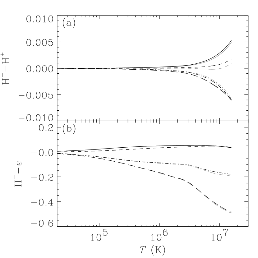
Figure 5: a) The relative change of $K$ (long-dashed line), $z$ (solid), $z^{\prime}$ (short-dashed) and $z^{\prime\prime}$ (dash-dotted) for $\mathrm{H}^{+}$-$\mathrm{H}^{+}$ collisions in the Sun in the sense (quantum - classical)/classical. For the dark line the quantum corrections tabulated by H71 have been utilized, while the grey lines were obtained with our fitting formulae (see Appendix B). b) As a), but for $\mathrm{H}^{+}$-$e$ collisions.

The excellent accuracy of our fitting formulae can be checked in Fig. 5, where the effect of the quantum corrections on the resistance coefficient and the thermal diffusion coefficients in the Sun is shown. The corrections increase toward the centre, and especially for the $\mathrm{H}^{+}$-$e$ collisions they considerably alter $K$. However, the diffusion velocity of H is basically determined by $\mathrm{H}^{+}$-$\mathrm{H}^{+}$ interactions and in that case the corrections for all quantities are below 1%. The expected weak influence on the solar structure is demonstrated by model S6, where our fitting formulae to the quantum corrections of H71 have been used. Overall, the diffusion velocities for all elements have been increased, more prominently in the centre, where the difference to models S5 (without quantum corrections) is the biggest (Fig. 5). This caused a further reduction of the sound-speed difference of model S6 compared to S5 (Fig. 3a).

It should be mentioned that the spin-dependent term in Eq. (13) would demand to know exactly the number of atoms in each ionization and in each excited state. However, the diffusion velocity of all elements is basically determined by their collision frequency with the most abundant element (H), and thus only for $\mathrm{H}^{+}$-$\mathrm{H}^{+}$ collision this spin-dependent term has to be accounted for (the spin-dependent term appears only in case of indistinguishable particles). Moreover, when quantum corrections become important inside stars most of the elements are already fully ionized. Thus only very tiny errors are introduced when, as in this work, only one mean-charged ion per element is considered.

It is interesting to notice that model S6, which includes the most accurate collision integrals of P86  accounts for the difference between repulsive and attractive interactions, and includes quantum effects, has almost the same sound-speed profile as model S1 (cf. Fig. 3a), which contains the most crude treatment of diffusion among all models considered in this work. Also the depth of the convective envelope and the surface helium content are nearly identical (Table 2). Therefore, just by chance, a very accurate solar model with respect to diffusion is obtained when using the resistance coefficients chosen by TBL.

4 Conclusions

In this paper, we have compared resistance coefficients computed by various groups for the calculation of atomic diffusion constants, and we have discussed the inclusion of quantum effects on the otherwise classical determination of these quantities. We provide simple analytical formulae to implement easily the presently most accurate determination of resistance coefficients, i.e., the classical result by P86 plus the effect of quantum corrections determined by H71. (FORTRAN routines for computing updated resistance coefficient and the consequent diffusion constants are publicly available.)

The different classical computations based on a a Debye-Hückel type of potential produce solar sound-speed profiles with significant differences when compared to the current accuracy of helioseismological determinations. Just by chance, our accurate treatment including quantum corrections produces a solar sound-speed profile comparable to the one obtained using the less accurate $z$, $z^{\prime}$ and $z^{\prime\prime}$ coefficients selected by TBL. In this context, we would like to add that with none of the descriptions for the collision integrals – neither with the inclusion of radiative levitation – the bump in the sound-speed difference at $r\approx 0.65\,R_{\odot}$ disappears. So, an additional mixing process beyond the formal boundary of the convective zones is still a probable candidate to resolve this discrepancy (see, e.g., Richard et al. 1996).

The introduction of quantum corrections increases the efficiency of diffusion with respect to the classical case, and their effect is more pronounced for higher densities. It will therefore be important to test the effect of our accurate resistance coefficients on models of objects denser than the Sun, like white dwarfs, and main sequence turn-off stars of galactic globular clusters, where also radiative levitation is altering the surface abundance patterns (Richard et al. 2002).

Although the accuracy of the diffusion constants could be improved considerably when using the correct functions for the resistance coefficients, there still remains the limitation that Burgers’ formalism is equivalent only to Chapman & Cowling’s (1970) second approximation. This causes an intrinsic uncertainty when using Burgers’ equation of the order of 10% (Roussel-Dupré 1982), which is difficult to reduce further.

Appendix A

In this appendix we provide analytic formulae for ${T^{\ast}}^{2}\,{\Omega^{(s,t)}}^{\ast}$ and those combinations of the indices $s$ and $t$ which are needed to compute the resistance coefficients $K$, $z$, $z^{\prime}$ and $z^{\prime\prime}$ using Eq. (1)–(4). The polynomial functions for the classical case have been obtained by a least square-difference fitting of the results of P86.

The best fits for the classical collision integrals could be obtained with

$${T^{\ast}}^{2}\,{\Omega^{(s,t)}}^{\ast}=\sum_{k=0}^{5}c^{\mathrm{A}}_{st}(k)\,\Phi^{k}$$ (14)

for attractive and

$${T^{\ast}}^{2}\,{\Omega^{(s,t)}}^{\ast} = \sum_{k=0}^{3}c^{\mathrm{R}}_{st}(k)\,(\tilde{\Phi}_{st})^{k}\quad\mbox{with}$$ (15)

$$\tilde{\Phi}_{st} = \ln\left(\ln(1+\Lambda^{b_{st}})\right)$$ (16)

for repulsive potentials. We dropped the indices $i,j$ for the sake of clarity. The numerical values for the coefficients $c^{\mathrm{A}}$ and $c^{\mathrm{R}}$, and the exponents $b$ are summarized in Table 3. Notice that it is sufficient to determine ${T^{\ast}}^{2}\,{\Omega^{(s,t)}}^{\ast}$, as in the definitions of the resistance coefficients the factor ${T^{\ast}}^{2}$ always cancels out.

Table 3: Coefficients for Eqs. (14)–(16).

	(s,t)
	(1,1)	(1,2)	(1,3)	(2,2)
$c^{\mathrm{A}}$(0)	$-$1.577	$-$2.062	$-$2.472	$-$1.776
$c^{\mathrm{A}}$(1)	0.6285	0.5066	0.4452	0.8555
$c^{\mathrm{A}}$(2)	0.08141	0.05224	0.04911	0.07976
$c^{\mathrm{A}}$(3)	0.03769	0.03302	0.02851	0.01198
$c^{\mathrm{A}}$(4)	$-$0.002702	$-$0.0005197	$1.605\!\times\!10^{-5}$	$-$0.002642
$c^{\mathrm{A}}$(5)	$-$0.001587	$-$0.001291	$-$0.001014	$-$0.0004393
$c^{\mathrm{R}}$(0)	$-$1.862	$-$2.465	$-$2.857	$-$1.702
$c^{\mathrm{R}}$(1)	2.313	1.667	1.386	1.916
$c^{\mathrm{R}}$(2)	$-$0.1550	$-$0.07154	$-$0.05136	$-$0.08114
$c^{\mathrm{R}}$(3)	$-$0.07188	$-$0.03209	$-$0.01620	$-$0.04868
$b$	0.6339	0.8228	0.9231	0.7807

The quantum-mechanical (“qu”) and exchange contribution (“ex”) can both be computed according to the following relationship

$${T^{\ast}}^{2}{\Omega^{(p,q)}_{\mathrm{qu,ex}}}^{\ast}(T^{\ast}\!{\Lambda^{\ast}}^{2}) = \frac{pN_{p}}{q(q+1)}\,I^{(q)}_{\mathrm{qu,ex}}(T^{\ast}\!{\Lambda^{\ast}}^{2})\quad\mbox{with}$$ (17)

$$N_{p}^{-1} = 1-\frac{1+(-1)^{p}}{2(1+p)}.$$ (18)

In these formulae the quantum and exchange parts of the collision integrals are expressed as functions of the quantity $T^{\ast}\!{\Lambda^{\ast}}^{2}$. The best fits to the values tabulated in H71 have been obtained with

$$I^{(q)}_{\mathrm{C}}(x) = \sum_{i=0}^{4}d_{\mathrm{C}}^{(q)}(i)\,{\xi_{\mathrm{C}}^{(q)}}^{i}(x)\mbox{,\quad where}$$ (19)

$$\xi_{\mathrm{C}}^{(q)}(x) = \left\{\begin{array}[]{lcl}\ln(1+g_{\mathrm{C}}^{(q)}\!\times\!x)&\mbox{for}&\mathrm{C}=\mbox{``qu''}{\rm,}\\ \ln(1+g_{\mathrm{C}}^{(q)}\;/\;x)&\mbox{for}&\mathrm{C}=\mbox{``ex''}{\rm}\\ \end{array}\right.$$ (22)

with $x=T^{\ast}\!{\Lambda^{\ast}}^{2}$ and the additional constraint that $\xi^{(q)}_{\mathrm{ex}}(x)=0$ for $x\leq 0.1$. The index “C” denotes the appropriate expression for either the quantum or the exchange contribution to the collision integrals. The respective coefficients are provided in Table 4. Note that $I^{(1)}_{\mathrm{ex}}=0$ and that Eqs. (19) and (22) are only valid for $x<1\,000$, as no values were provided by H71 for larger $x$. We suggest not to extrapolate $T^{\ast}\!{\Lambda^{\ast}}^{2}$ beyond this upper boundary, but to use the values at $T^{\ast}\!{\Lambda^{\ast}}^{2}=1\,000$, which are $I^{(2)}_{\mathrm{ex}}=0.4913$, $I^{(3)}_{\mathrm{ex}}=0.4960$, $I^{(1)}_{\mathrm{qu}}=1.5053$, $I^{(2)}_{\mathrm{qu}}=1.9581$ and $I^{(3)}_{\mathrm{qu}}=2.2010$.

Table 4: Coefficients for Eqs. (19)–(22)

	$q$
	1	2	3
$d_{\mathrm{ex}}(0)$	—	$-$0.7074	$-$0.7103
$d_{\mathrm{ex}}(1)$	—	$-$1.985	$-$2.744
$d_{\mathrm{ex}}(2)$	—	0.5233	0.1870
$d_{\mathrm{ex}}(3)$	—	$-$0.3270	0.03388
$d_{\mathrm{ex}}(4)$	—	0.03920	$-$0.06502
$d_{\mathrm{qu}}(0)$	0	0	0
$d_{\mathrm{qu}}(1)$	0.05333	0.03051	0.3133
$d_{\mathrm{qu}}(2)$	0.01889	0.01021	0.03982
$d_{\mathrm{qu}}(3)$	0.007114	0.009180	$-$0.003032
$d_{\mathrm{qu}}(4)$	$-$0.0006953	$-$0.0007776	$1.388\!\times\!10^{-5}$
$g_{\mathrm{ex}}$	—	6.121	2.285
$g_{\mathrm{qu}}$	0.3	1.0	0.15

Appendix B

Here we describe the modifications to be applied to the routine by TBL, in order to use any preferred formulation of the resistance coefficients.

The first change involves Eqs. (9)–(10) of TBL, where the IM85 definition of $K$ is implemented. They have to be replaced with the chosen representation of $K$.

The matrix of elements $Y_{st}$, introduced at page 830 of TBL, has to be changed to

$$Y_{st}=3y_{st}+z^{\prime}_{st}\,x_{st}\,m_{t}/m_{s}.$$ (23)

Finally, the following elements of the matrix $\Delta_{ij}$ as defined in Eqs. (33) and (34) of TBL become

$$\Delta_{ij}=\left\{\begin{array}[]{lcl}\sum_{k\neq i}z_{ik}k_{ik}x_{ik}&\mbox{for}&j=i+S{\rm,}\\[6.0pt] -z_{iq}\,k_{iq}\,y_{iq}&\mbox{for}&j=S+1,\dots,2S\\ &&\mbox{and\leavevmode\nobreak\ }j\neq i+S{\rm,}\\ \end{array}\right.$$ (24)

for $i=1,\dots,S$ and

$$\Delta_{ij}=\left\{\begin{array}[]{lcl}2.5\sum_{k\neq j}z_{pk}k_{pk}x_{pk}&\mbox{for}&j=p{\rm,}\\[6.0pt] -2.5z_{pj}k_{pj}x_{pj}&\mbox{for}&j=1,\dots,S\mbox{\leavevmode\nobreak\ and\leavevmode\nobreak\ }j\neq p{\rm,}\\[6.0pt] \lx@intercol\@ADDCLASS{ltx_eqn_lefteqn}$\displaystyle-{\textstyle\sum_{k\neq i}}k_{pk}y_{pk}(0.8z^{\prime\prime}_{pk}x_{pk}+Y_{pk})-0.4z^{\prime\prime}_{pp}k_{pp}$\mbox{}\hfil\lx@intercol\\ &\mbox{for}&j=i{\rm,}\\[6.0pt] \lx@intercol\@ADDCLASS{ltx_eqn_lefteqn}$\displaystyle k_{pq}y_{pq}x_{pq}(3+z^{\prime}_{pq}-0.8z^{\prime\prime}_{pq})$\mbox{}\hfil\lx@intercol\\ &\mbox{for}&j=S+1,\dots,2S\\ &&\mbox{and\leavevmode\nobreak\ }j\neq i{\rm,}\end{array}\right.$$ (32)

for $i=S+1,\dots,2S$, where $p=i-S$ and $q=j-S$. Here, the same symbols have been used as in TBL, to which the reader is referred for their definitions.

References

- Bahcall et al. (1998) Bahcall, J. N., Basu, S., & Pinsonneault, M. H. 1998, Phys. Lett. B, 433, 1
- Bahcall et al. (1995) Bahcall, J. N., Pinsonneault, M. H., & Wasserburg, G. J. 1995, Rev. Mod. Phys., 67, 781
- Basu & Antia (1995) Basu, S. & Antia, H. M. 1995, MNRAS, 276, 1402
- Basu & Antia (1997) —. 1997, MNRAS, 287, 198
- Basu et al. (1997) Basu, S., Chaplin, W. J., Christensen-Dalsgaard, J., et al. 1997, MNRAS, 292, 243
- Bonifacio et al. (2002) Bonifacio, P., Pasquini, L., Spite, F., et al. 2002, A&A, 390, 91
- Burgers (1969) Burgers, J. M. 1969, Flow Equations for Composite Gases (New York, London: Academic Press) (B69)
- Chapman & Cowling (1970) Chapman, S. & Cowling, T. G. 1970, The Mathematical Theory of Non-Uniform Gases, 3rd edn. (Cambridge University Press)
- Gratton et al. (2001) Gratton, R. G., Bonifacio, P., Bragaglia, A., et al. 2001, A&A, 369, 87
- Hahn et al. (1971) Hahn, H.-S., Mason, E. A., & Smith, F. J. 1971, Phys. Fluids, 14, 278 (H71)
- Hirschfelder et al. (1954) Hirschfelder, J. O., Curtiss, C. F., & Bird, R. B. 1954, Molecular Theory of Gases and Liquids (New York: John Wiley & Sons, Inc.)
- Iben & MacDonald (1985) Iben, I., jr. & MacDonald, J. 1985, ApJ, 296, 540 (IM85)
- Mason et al. (1967) Mason, E. A., Munn, R. J., & Smith, F. J. 1967, Phys. Fluids, 10, 1827 (MMS67)
- Michaud et al. (1984) Michaud, G., Fontaine, G., & Beaudet, G. 1984, ApJ, 282, 206
- Muchmore (1984) Muchmore, D. 1984, ApJ, 278, 769 (M84)
- Paquette et al. (1986) Paquette, C., Pelletier, C., Fontaine, G., & Michaud, G. 1986, ApJS, 61, 177 (P86)
- Richard et al. (2002) Richard, O., Michaud, G., Richer, J., et al. 2002, ApJ, 568, 979
- Richard et al. (1996) Richard, O., Vauclair, S., Charbonnel, C., & Dziembowski, W. A. 1996, A&A, 312, 1000
- Roussel-Dupré (1982) Roussel-Dupré, R. 1982, ApJ, 252, 393
- Schlattl (2002) Schlattl, H. 2002, A&A, 395, 85
- Thoul et al. (1994) Thoul, A. A., Bahcall, J. N., & Loeb, A. 1994, ApJ, 421, 828 (TBL)
- Turcotte et al. (1998) Turcotte, S., Richer, J., Michaud, G., Iglesias, C. A., & Rogers, F. J. 1998, ApJ, 504, 539
- Vauclair & Charbonnel (1995) Vauclair, S. & Charbonnel, C. 1995, A&A, 295, 715