Intercalibration of Cherenkov Telescopes in Telescope Arrays

Abstract

A simple analysis technique is described which allows to intercalibrate the response of imaging atmospheric Cherenkov telescopes in stereoscopic telescope arrays at a level of 1-2%.

With the next-generation imaging atmospheric Cherenkov telescopes currently under construction, stereoscopic arrays of telescopes such as VERITAS [1], CANGAROO III [2] and H.E.S.S. [3] play a dominant role. Stereoscopic systems of Cherenkov telescopes for VHE gamma-ray astrophysics provide - compared to a single telescope - superior angular resolution, energy resolution and background rejection, as demonstrated by the HEGRA group [4, 5]. Making use of information concerning the impact point of showers and the height of the shower maximum, energy resolutions around 10% are possible [6]. To actually obtain this resolution, the relative response of the telescopes, i.e. the relation between the light yield and the digital counts provided by the ADC system must be known with very good precision. Photon detectors within one telescope can be flat-fielded using a light pulser in the center of the dish. Telescope-to-telescope intercalibration is more complicated, and recently e.g. the use of cosmic ray trigger rates and the so-called throughput method has been advocated for this purpose [7]. In the following, a simple technique for telescope intercalibration is discussed (see also [8]).

Once a telescope is properly flat-fielded, one needs only one global calibration factor per telescope, relating the image size - the sum of the amplitudes of all image pixels - to the photon yield, up to some overall calibration factor common to all telescopes of an array. The response of two telescopes can be compared by selecting showers with cores in the middle between two telescopes, and comparing the image sizes of both telescopes. However, in systems with more than two telescopes, one needs to be careful not to introduce a bias due to other telescopes involved in the triggering or the event reconstruction. Testing the technique with the HEGRA telescope system, the following procedure was followed:

• To compare the response of two telescopes, events were selected where both telescopes under consideration had triggered (and possible others in addition)

• Only information from the two telescopes under consideration was used in reconstruction the shower; images from other telescopes were ignored.

• To reduce the influence of trigger thresholds, a cut well above the threshold was applied; the sum of the image sizes of the two telescopes had to be above 200 photoelectrons.

• To improve image quality and reconstruction, only images within a radius of $1.75^{\circ}$ from the camera center were used, avoiding image truncation. The (stereo) angle between the two image axes had to be at least $30^{\circ}$. Reconstructed shower directions had to be within $0.7^{\circ}$ from the telescope axis.

The relative response of two telescopes $i$ and $j$ was then characterized by plotting the size asymmetry $a_{s}$ versus the asymmetry $a_{r}$ in impact distance (Fig. 1), where

$$a_{s(ij)}={s_{i}-s_{j}\over s_{i}+s_{j}}$$

and

$$a_{r(ij)}={r_{i}-r_{j}\over r_{i}+r_{j}}$$

Here, $s_{i}$ is the image size in telescope $i$ and $r_{i}$ its distance to the reconstructed shower impact point, measured perpendicular to the shower axis. The asymmetry parameters were chosen because they treat both telescopes in a symmetrical fashion; one could also use $\log(s_{i}/s_{j})$ or similar quantities.

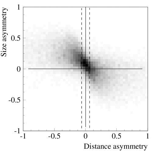
Figure 1: Distribution of size asymmetry $a_{s}$ versus distance asymmetry $a_{r}$, for a telescope pair of the Mkn 501 data set. The dashed lines indicate the cut range used to derive $a_{s}(a_{r}\approx 0)$.

To evaluate the relative response of the two telescopes, one needs to determine the average $a_{s}$ for $a_{r}=0$. This can be achieved by averaging $a_{s}$ for bins of $a_{r}$ and then fitting a smooth curve to $<a_{s}(a_{r})>$, or, if event statistics is high enough, by simply cutting on $a_{r}$. For the following examples, the mean value of $a_{s}(a_{r}\approx 0)$ were obtained by fitting a Gaussian to the distribution of $a_{s}$ for $|a_{r}|<0.05$. The method was first applied to Monte-Carlo simulations of the HEGRA telescope system in its 1997 configuration, with four telescopes; one of the outer telescopes was still incomplete. In the simulation, the response of the four telescopes (for historical reasons labelled CT3, CT4, CT5, CT6) was adjusted as 1 : 0.8 : 1.1 : 1.3. The “measured” size asymmetries are listed in the following table; the last column gives the values expected on the basis of the input response factors.

Telescopes	asymmetry	true value
	$\pm 0.002$
CT3-CT4	0.113	0.111
CT3-CT5	-0.052	-0.048
CT3-CT6	-0.128	-0.130
CT4-CT5	-0.160	-0.158
CT4-CT6	-0.242	-0.238
CT5-CT6	-0.082	-0.082

From the first three lines, one readily determines a relative response of the telescopes to 1 : 0.797 : 1.109 : 1.292 , in agreement with the input values to better than 1%. With six measurements for three independent quantities (arbitrarily defining the response factor for CT3 as unity), one should determine optimum calibration factors by a fit to all measurements; such a fit yields response ratios of 1 : 0.797 : 1.104 : 1.300, with typical errors of 0.003 and a $\chi^{2}$ of 5.2 for 3 degrees of freedom, indicating that small systematic effects may be present beyond the statistical errors.

The method was then applied to actual HEGRA data, from observations of Mkn 501 in 1997. Two independent data samples were considered, (a) a background-subtracted gamma-ray sample obtained by cutting on the mean scaled width of images and on the reconstructed direction relative to the source, and (b) a cosmic-ray sample. The measured asymmetries are given in the following table:

Telescopes	sample (a)	sample (b)
	$\pm 0.006$	$\pm 0.003$
CT3-CT4	0.033	0.021
CT3-CT5	0.071	0.073
CT3-CT6	0.117	0.114
CT4-CT5	0.037	0.039
CT4-CT6	0.089	0.084
CT5-CT6	0.023	0.045

Fits for the telescope response factors yield

sample (a): CT3 : CT4 : CT5 : CT6 = 1 : 0.937 : 0.857 : 0.797

sample (b): CT3 : CT4 : CT5 : CT6 = 1 : 0.948 : 0.872 : 0.798

with typical errors of 0.01 for sample (a) and 0.005 for sample (b). The results are consistent within errors; the $\chi^{2}$ values for the fits are 9.7 and 7.5, again slightly worse than expected for purely statistical errors.

In summary, the method allows an easy intercalibration of imaging atmospheric Cherenkov telescopes in a telescope system. Both the simulations and the comparison of two independent data samples shows that a precision of 1-2% can be reached, which is ample even for a 10% overall energy resolution. For systems with more than two telescopes, the equation system is overdetermined and consistency checks are possible, e.g. in the form of the $\chi^{2}$ value of an overall fit. The method can be applied to systems with arbitrary numbers of telescopes, provided that they do not separate into multiple distant clusters of telescopes. The absolute calibration for the whole system can be determined in a subsequent step, e.g., using cosmic-ray detection rates (see, e.g. [7, 9]).

Acknowledgements. The support of the German Ministry for Education and Research BMBF is acknowledged. The author is grateful to the members of the HEGRA collaboration, who have participated in the development, installation, and operation of the telescopes, and in the data precessing.

References

- [1] T.C. Weekes et al., Astropart. Phys. 17 (2002) 221
- [2] R. Enemoto et al., Astropart. Phys. 16 (2002) 235
- [3] W. Hofmann, Proc. of the Int. Cosmic Ray Conf., Hamburg, 2001, M. Simon, E. Lorenz, M. Pohl (Eds), Vol. 7, 2785
- [4] A. Daum et al., Astropart. Phys. 8 (1997) 1
- [5] A. Konopelko et al., Astropart. Phys. 10 (1999) 275
- [6] W. Hofmann, H. Lampeitl, A. Konopelko, H. Krawczynski, Astropart. Phys. 12 (2000) 207
- [7] S. LeBohec, J. Holder, astro-ph/0208396 (2002)
- [8] W. Hofmann, Proc. “Towards a Major Atmospheric Cherenkov Detector V”, Kruger Park, 1997, O.C. de Jager (Ed.), p. 284
- [9] A. Konopelko et al., Astropart. Phys. 4 (1996) 199