First Results from the HI Jodrell All Sky Survey: Inclination-Dependent Selection Effects in a 21-cm Blind Survey

Abstract

Details are presented of the HI Jodrell All Sky Survey (HIJASS). HIJASS is a blind neutral hydrogen (HI) survey of the northern sky ($\delta$$>$22°), being conducted using the multibeam receiver on the Lovell Telescope (FWHM beamwidth 12 arcmin) at Jodrell Bank. HIJASS covers the velocity range –3500 km s^-1 to 10000 km s^-1, with a velocity resolution of 18.1 km s^-1 and spatial positional accuracy of $\sim$2.5 arcmin. Thus far about 1115 deg² of sky have been surveyed. The average rms noise during the early part of the survey was around 16 mJy beam^-1. Following the first phase of the Lovell telescope upgrade (in 2001), the rms noise is now around 13 mJy beam^-1. We describe the methods of detecting galaxies within the HIJASS data and of measuring their HI parameters. The properties of the resulting HI-selected sample of galaxies are described. Of the 222 sources so far confirmed, 170 (77 per cent) are clearly associated with a previously catalogued galaxy. A further 23 sources (10 per cent) lie close (within 6 arcmin) to a previously catalogued galaxy for which no previous redshift exists. A further 29 sources (13 per cent) do not appear to be associated with any previously catalogued galaxy. The distributions of peak flux, integrated flux, HI mass and $cz$ are discussed. We show, using the HIJASS data, that HI self-absorption is a significant, but often overlooked, effect in galaxies with large inclination angles to the line of sight. Properly accounting for it could increase the derived HI mass density of the local Universe by at least 25 per cent. The effect this will have on the shape of the HI Mass Function (HIMF) will depend on how self-absorption affects galaxies of different morphological types and HI masses. We also show that galaxies with small inclinations to the line of sight may also be excluded from HI-selected samples, since many such galaxies will have observed velocity-widths which are too narrow for them to be distinguished from narrow-band radio frequency interference. This effect will become progressively more serious for galaxies with smaller intrinsic velocity-widths. If, as we might expect, galaxies with smaller intrinsic velocity-widths have smaller HI masses, then compensating for this effect could significantly steepen the faint-end slope of the derived HIMF.

1 Introduction

A complete and bias-free census of the population of extragalactic objects is essential to any study of the formation and evolution of galaxies or the large-scale structure of the universe. However, our current understanding of galaxy populations has been primarily derived from optical and IR surveys. There is an inevitable bias in such surveys against low luminosity objects (dwarfs), but also against low surface brightness (LSB) objects (see, e.g. Disney 1976; Disney & Phillipps 1987; Impey & Bothun 1997; Disney 1999).

However, it has become clear that low luminosity and low surface brightness galaxies play a key role in many cosmological and cosmographical problems. For example, dwarf/LSB galaxies can clearly play a major role in helping us to understand large-scale structure and its influence on galaxy formation and evolution. Their numbers and distribution place constraints on the increasingly sophisticated numerical and semi-analytic models of galaxy formation (e.g., Baugh, Cole & Frenk 1996; Kauffmann et al. 1997), while their morphologies and stellar contents may reflect the local physics which define the star formation process in galaxies (e.g., Bell & Bower 2000; Bell & de Jong 2000).

Recent observational studies have fully supported the view (expounded by, e.g., Phillipps et al. 1987 and Impey, Bothun & Malin 1988) that low luminosity and low surface brightness galaxies numerically dominate the galaxy population in the local Universe (see e.g. McGaugh 1996; Cross et al. 2001). However, optical surveys of the local Universe for faint/LSB objects are problematic due to the very long exposure times required, the large areas which need to be surveyed and the need to measure a redshift for each faint/LSB object found. Consequently, our knowledge of the local population of galaxies at low luminosity and low surface brightness is still relatively limited. This inhibits our knowledge of many broader cosmological/cosmographical issues.

Given the limitations of optical surveys for detecting low luminosity / LSB objects, an alternative method to sample the extragalactic population is to use the 21-cm neutral hydrogen (HI) line. This provides a way of potentially circumventing optical selection effects operating against low luminosity and/or LSB objects, since a galaxy’s HI content may be relatively uncorrelated with its optical emission. For example, it is well known that elliptical galaxies contain little HI whereas we might expect to find large amounts of HI in galaxies where star formation has been inefficient, e.g. in low luminosity and LSB galaxies. However, until comparatively recently, most HI surveys were limited to HI measurements of galaxies previously detected in optical or IR surveys. The advent of the 21-cm multibeam receiving systems at Parkes and Jodrell Bank has made possible, for the first time, blind HI surveys of large areas of sky to reasonable sensitivity over comparatively large volumes.

The HI Parkes All Sky Survey (HIPASS, Staveley-Smith et al. 1996) was commenced in 1997 and concluded in 2002. HIPASS has surveyed the southern hemisphere (up to $\delta$=+25°) to $cz$=12700 km s^-1 and an HI mass limit around 10⁶d${}^{2}_{\rm Mpc}$ M_⊙. Results from HIPASS have indeed added significantly to the census of the local extragalactic population. Recent scientific highlights include the discovery of 10 new members to the Cen A group (Banks et al. 1999), the detection of an apparently extragalactic HI cloud with no optical counterpart to faint limits (Kilborn et al. 2000) and the discovery of a massive HI cloud associated with NGC 2442 (Ryder et al. 2001). Kilborn et al. (2002) have recently published a catalogue of 536 galaxies from a 2400 sq deg region of HIPASS covering the South Celestial Cap. Koribalski et al. (in preparation) will present the HIPASS Brightest Galaxies Catalogue (BGC), a catalogue of the brightest 1000 galaxies (in terms of HI peak flux) from the whole of HIPASS. Meanwhile, Ryan-Weber et al. (2002) have discussed the properties of those previously uncatalogued galaxies found in the BGC.

The HI Jodrell All Sky Survey (HIJASS) is the northern counterpart to HIPASS. HIJASS will survey the northern sky above $\delta$=22°  to similar sensitivity to HIPASS, using the Multibeam 4-beam cryogenic receiver mounted on the 76-m Lovell Telescope. HIJASS was begun in 2000. So far $\simeq$1115 deg² have been surveyed. We recently presented results from the HIJASS data covering the M81 group (Boyce et al. 2001). The survey reveals several new aspects to the complex morphology of the HI distribution in the group and illustrates that a blind HI survey of even such a nearby, well studied group of galaxies can add much new information.

This paper presents a detailed description of the HI Jodrell All Sky Survey and of the properties of the HI-selected sample of galaxies which has been compiled so far from the HIJASS data. We use the sample of confirmed HIJASS sources to study the effect that a galaxy’s inclination to the line of sight has on its inclusion within an HI-selected sample. We show that both highly inclined galaxies and galaxies close to face-on are subject to selection effects which could have led to their being under-represented in previous determinations of the HI Mass Function (HIMF) and HI mass density, $\Omega_{\rm HI}$, from HI-selected samples of galaxies.

Section 2 describes the hardware, the observing strategy and survey parameters and also describes the data reduction methods. Section 3 describes the methods by which galaxies have been detected within HIJASS data and their parameters measured. Section 4 is a discussion of the properties of the sample of galaxies found in HIJASS data thus far. In Section 5 we use the sample of confirmed HIJASS sources to study the inclination-dependent selection effects on the inclusion of a galaxy in an HI-selected sample and discuss the implications of this. Section 6 presents some concluding remarks.

2 The Survey

2.1 Hardware

HIJASS uses a cryogenic Multibeam receiver (Bird 1997) of similar design to the Multibeam receiver used at Parkes for HIPASS (Staveley-Smith et al. 1996). The Multibeam system installed at Jodrell Bank has four dual linearly polarised receivers covering a frequency range of 1200 MHz to 1550 MHz. The feed horn array consists of 4 stepped circular horns (which were designed at the CSIRO) arranged in a rhombic pattern, the apertures of which are located at the telescope prime focus. Stepped circular horns were chosen because of their good pattern symmetry, low spillover and good cross polarization properties (Bird 1994). The horns couple directly into a low temperature, high vacuum, cryogenic dewar. The output from the feed horn arrays are then fed to a set of 3-stage high electron mobility transistor (HEMT) pre-amplifiers which are cooled to a temperature of around $\sim$25 K. Following amplification, each receiver RF band is then down converted to an IF bandpass which can be set anywhere between 30 MHz and 245 MHz.

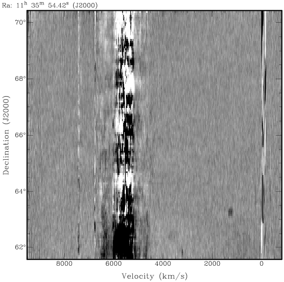
Figure 1: A section of a HIJASS cube at roughly constant $R.A.$. Visible are the residue of Galactic HI at 0 kmṡ^-1, the galaxy UGC06534 at $V_{\odot}\simeq$1300 km s^-1; and the radio frequency interference between 4500$\rightarrow$7500 km s^-1.

Each of the 8 resultant IF bands are then passed from the focus cabin to the observing room via about 300 m of low loss coaxial cable which is terminated into N-socket connections in the Lovell Observing Room. These outputs are next patched into a set of digitally programmable attenuators and are then fed into a set of equaliser and splitter units. Each IF is equalised for frequency dependent cable losses and then split into two outputs. The first output connects to a filter bank which sets the bandpass which is presented to the correlator. A second set of outputs are used for pulsar survey measurements.

The correlator was constructed at the Australia Telescope National Facility (ATNF). It is built around special purpose VLSI chips developed by the NASA Space Engineering Research Centre for VLSI System Design (Canaris 1993). These chips accept 2-bit sampled data streams at rates of up to 140 Msamples/sec and form either the cross correlation function of the two streams or the autocorrelation function of one stream at 1025 contiguous sample delays. The chip has 1024 32-bit accumulators and a 32-bit output bus and can integrate for up to 16 seconds. In the multibeam correlator, one of these chips, operating in autocorrelation mode, is used on each of the 8 sampled data streams, thereby providing, after Fourier transformation, a measurement of the input spectrum at 1024 contiguous frequencies spaced at 62.5 kHz (equivalent to 13.2 km s^-1 at the rest frequency of HI).

2.2 Observing strategy and data reduction

The survey is conducted by actively scanning the sky in 8°  strips in Declination, at a rate of 1°  per minute. Each declination scan is separated by 10 arcmin but each area of sky is scanned 8 times, resulting in a final scan separation of 1.25 arcmin. The data from the 8 correlators are stored every 5 s. A 64 MHz bandpass with 1024 channels is used, although local interference at the band edges restricts the useful velocity range to about –1000 km s^-1 to +10000 km s^-1 (note, however, that a broad band of radio frequency interference also affects all velocities between 4500 km s^-1 and 7500 km s^-1 - see Section 2.3). The system temperature is $\sim$30 K. Bandpass correction and calibration are applied using the software package LIVEDATA (see Barnes et al. 2001). The spectra are gridded into three-dimensional 8°$\times$8°  datacubes ($\alpha$,$\delta$,$V_{\odot}$) using the software package GRIDZILLA (Barnes et al. 2001). The observed spectra are smoothed online by applying a 25 per cent Tukey filter to reduce ‘ringing’ caused by strong Galactic signals entering through the side-lobes. This reduces the actual velocity resolution in the gridded datacubes to 18.1 km s^-1. The spatial pixel size of the datacubes is 4 arcmin$\times$4 arcmin. The effects of continuum emission on the baselines of the spectra in each cube are then removed by the program POLYCON written by Daniel Zambonini and Robert Minchin. This program fits and then subtracts a 5th order polynomial baseline to each individual spectrum in a datacube: fitting is only performed on parts of the spectrum free of interference or line emission.

2.3 Areas Surveyed and Data Quality

HIJASS has been conducted during three observing runs: in April-June 2000; in Jan-Feb 2001; and in Jan 2002. Table 1 notes those areas of the northern sky so far surveyed by HIJASS and during which run the data were taken. The whole of a strip in R.A. between Decl.=70°$\rightarrow$78°  has been surveyed (795 deg²). Two areas of the R.A. strip between Decl.=62°$\rightarrow$70°have also been surveyed (192 deg²), along with smaller areas at Decls.=58°, 34°, and 26°. In total 1115 deg² has been surveyed thus far.

Table 1: Areas surveyed by HIJASS

Decl. Range	R.A. Range	Area (deg2)	Run
70°–78°	complete	795	2000,2001
62°–70°	09h02m–11h55m	128	2001,2002
	02h30m–04h02m	64	2002
54°–62°	03h26m–04h08m	32	2001
30°–38°	01h13m–01h59m	64	2002
22°–30°	12h08m–12h34m	32	2002

Fig. 1 shows an example of the data. This is a plot of Decl. against Velocity at roughly constant R.A.. The HIJASS source HIJASS J1133+63 can be seen at Decl.$\simeq$63°, $V_{\odot}$=1300 km s^-1. This has been identified as UGC 06534. Prominent in the data is a broad band of radio frequency interference (RFI) which affects all velocities from $\simeq$4500 km s^-1 to 7500 km s^-1. This is mainly due to off-site radio and data communication emissions generated in the locality.

Between the observing runs in 2001 and 2002, the Lovell dish underwent the first stage of a major upgrade. A new telescope drive system was installed and around half of the dish surface was replaced.

Prior to this upgrade, the rms noise in the datacubes (away from the broad-band RFI) was typically 16-18 mJy beam^-1. However, those cubes made from data taken following the first stage of the refurbishment (i.e. in 2002), show an improvement in sensitivity by around 25 per cent, the rms noise in these cubes being about 12-14 mJy beam^-1. The improvement is believed to be due to a combination of several factors: the improved sensitivity of the partially resurfaced dish, an improvement in the telescope pointing model, an improvement in the smoothness of the scanning and a concerted effort to reduce local (Jodrell-based) interference during the observing run.

3 Detecting and Parametrizing Galaxies in HIJASS Data

3.1 Galaxy detection techniques

The general method of detecting galaxies in the HIJASS data is as follows. An initial candidate galaxy list is formed by visually searching the datacubes. The visual display program KVIEW (Gooch 1995) is used to search through the data in three dimensions by displaying 2 axes and stepping through the third. Narrow velocity-width, bright galaxies are most easily seen when the data are displayed in R.A. versus Decl. and stepped through Velocity. Broad velocity-width, faint galaxies are more easily discovered when the datacube is displayed R.A. or Decl. versus Velocity. The selection criteria for this visual sample is that a detection must : (1) be easily visible above the noise ($\sim$3$\sigma$ in peak flux), (2) should have a spatial extent of greater than 1 pixel, and (3) be visible over two or more velocity planes. Two lists are compiled using these criteria: one of ‘definite’ detections and one of ‘possible’ detections. The list of possible detections includes sources close to the selection limit or just below it but still considered possible sources.

A second candidate galaxy list is formed by running the automated finding algorithm POLYFIND, written by Robert Minchin and Jonathon Davies. POLYFIND determines the noise in non-masked regions of a hanning smoothed datacube and then looks for peaks at some user-defined level above the noise (typically set at 3$\sigma$). It then runs a series of matched filters over these identified peaks and a peak is noted as a potential source if a sufficiently good fit is obtained. The results from POLYFIND are then re-checked by eye using the same criteria as used for the eyeball method and lists of definite and possible detections made.

The two lists of definite detections are then amalgamated and these objects included in our final sample of confirmed HIJASS galaxies. The two lists of possible detections are also amalgamated. These objects are then re-observed with the Lovell telescope in single-beam mode using a bandwidth of 16 MHz. Those possible sources confirmed by this narrow-band follow-up are then added to the sample of confirmed HIJASS sources. The possible sources found during the 2002 run have not yet been subjected to narrow-band follow-up. Hence, for the 2002 data, only the definite detections found by the above selection methods have presently been included in the sample (69 sources).

3.2 Parametrization of the galaxies

The parameters of those galaxies included in the sample of confirmed HIJASS sources are determined from the data using tasks from the MIRIAD software package (Sault et al. 1995). Firstly, a two-dimensional Gaussian fit (IMFIT) is made to a zeroth order (intensity) moment-map of each detection to determine the central position of the galaxy as well as the spatial extent of the HI. The central position is then used to generate a spatially integrated spectrum of the detection, using a box size based on the extent of the HI. The spectrum is generated using MBSPECT which also gives a measurement of the peak and integrated flux of each detection, as well as the 50 per cent and 20 per cent velocity-width, the rms noise and barycentric velocity.

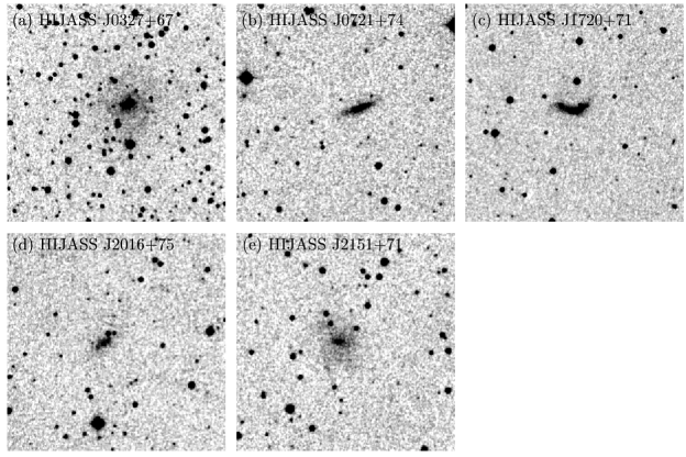
Figure 2: Digitial Sky Survey images of the 5 PUGs for which an obvious and umabiguious optical counterpart can be seen. Each image is 5 arcmin$\times$5 arcmin.

Table 2 presents the derived parameters for the sample of confirmed HIJASS sources. Column 1 gives the HIJASS Name. Columns 2 and 3 give the Right Ascension (J2000) and Declination (J2000) from the IMFIT task. Columns 4-6 list the zeroth order moment (Integrated flux S_Int=$\int S_{V}dV$), the peak flux ($S_{peak}$), and the noise (rms dispersion around the baseline, $\sigma$); all as measured by MBSPECT. Columns 7-9 give the first order moment (barycentric velocity V_⊙), the velocity width at 20 per cent of the peak flux ($\Delta$V₂₀), and the velocity width at 50 per cent of the peak flux ($\Delta$V₅₀), all measured by MBSPECT in the radio frame and converted to $cz$. The error in integrated flux is calculated from the rms noise on the spectrum and the velocity extent of the source.

Columns 10-13 contain the details of any counterpart to the HIJASS source, as listed in the NASA/IPAC Extragalactic Database (NED). Column 10 contains one of five possible classifications. If there is no object within NED which could be spatially coincident with the HIJASS source (defined as being within 6 arcmin), then Column 10 contains the classification ‘PUG’ (i.e. Previously Uncatalogued Galaxy). If there is an object in NED which matches the HIJASS source in both position and space (defined as being within 6 arcmin and 100 km s^-1) then this is listed as ‘ID’ (Identification). Those IDs which have been detected in HI for the first time by HIJASS are denoted by an asterix, i.e. ‘ID*’. If there is an object within NED which is spatially coincident with the HIJASS source (i.e. within 6 arcmin) but for which no redshift is listed in NED, then Column 10 contains the classification ‘ASS’ (i.e. Association). In several cases, there is more than one galaxy within 6 arcmin: in these cases the classification ‘ASS*’ is used. For the ID, ID* and ASS classifications, Column 11 lists the object within NED which appears to correspond to the HI detection. Column 12 lists the position offset (in arcmin) of the coordinates of the optical counterpart from the HI position. Column 12 lists (for the IDs and ID*s) the velocity offset of the barycentric velocity contained within NED from the barycentric velocity as measured by HIJASS.

4 Properties of the HIJASS galaxies

4.1 Composition of the sample

There are currently 222 sources included in the sample of confirmed HIJASS sources. Of these, 170 (77 per cent) are clearly associated with a previously catalogued galaxy (classification ID or ID*). However, 25 of these 170 objects have been detected in HI for the first time by HIJASS (classification ID*). For 4 of these 170 sources, HIJASS appears to be measuring HI from a pair or a small group of galaxies which lie at the redshift of the HI.

There are a further 23 HIJASS sources (10 per cent of the whole sample) which lie within 6 arcmin of a catalogued galaxy for which no redshift is reported in NED (classification ASS or ASS*). These HIJASS sources may or may not be associated with the catalogued galaxy. 15 of these sources have only one possible optical counterpart within 6 arcmin of the HI position (classification ASS). We may be relatively confident about the optical identification of these sources. However, even for these sources there remains the possibility that the HI has been detected from an associated HI cloud (cf. Ryder et al. 2001) or a LSB companion. The other 8 of the 23 sources have more than one galaxy within 6 arcmin of the HIJASS position (classification ASS*). We intend to obtain accurate positions for all 23 of these sources using HI aperture synthesis observations, so as to unambiguously determine the optical counterpart of each source.

There are then a further 29 sources (13 per cent of the whole sample) which do not lie within 6 arcmin of any previously catalogued galaxy (classification PUG). A study of the Digital Sky Survey (DSS) at the positions of these sources reveals an obvious and unambiguous optical counterpart in only 5 cases (J0327+67, J0721+74, J1720+71, J2016+75 and J2151+71). Fig. 2 presents the DSS images of these five PUGs. Three of these objects (J0327+67, J2016+75, J2151+71) have a compact but relatively high surface brightness core but a low surface brightness disk. They may have been excluded from optical catalogues because they were mistaken for stars. One object (J0721+74) is a highly inclined but relatively high surface brightness object, although very small ($\simeq$1 arcmin diameter). The fifth object (J1720+71) has a complex morphology and appears to be involved in some kind of interaction or merger.

A study of the DSS for the other 24 PUGs, reveals no unambiguous optical counterpart. In many cases there are several possible optical candidates within the positional uncertain of HIJASS. In several cases, however, no possible candidate can be seen. The optical counterparts of these sources must be of very low surface brightness. All of the PUGs will have accurate positions determined from aperture synthesis observations and will be the subject of deep optical follow-up work.

It is interesting to compare the number of PUGs found in the sample of confirmed HIJASS sources with those found in the Bright Galaxy Catalogue (BGC: Koribalski et al., in preparation). The BGC contains the 1000 brightest (in HI peak flux) sources in the whole of the HIPASS sample. 87 of these objects had not been previously catalogued, although 57 of these lie close (within 10$\,{}^{\circ}$) to the Galactic plane. Of the other 30 previously uncatalogued galaxies within the BGC, Ryan-Weber et al. (2002) found a single optical counterpart for 25 on the DSS. Whilst the relative number of previously uncatalogued galaxies within the BGC is much smaller than within the HIJASS sample (3 per cent compared to 13 per cent), most of the BGC objects can be unambiguously assigned to an optical counterpart on the DSS, whilst most of the HIJASS PUGs cannot be. These differences are probably primarily due to the different flux limits of the two samples. The faintest source in the BGC has a peak flux of 116 mJy. Only 6 of the 29 HIJASS PUGs have a peak flux larger than this. The much lower peak flux limit of HIJASS has produced a much larger fraction of PUGs compared to the BGC. Since these have generally lower HI flux, they are correspondingly harder to detect in optical data.

As it currently stands, the sample of confirmed HIJASS sources presents the first HI measurement of 77 galaxies (i.e. classes ID*, ASS, ASS*, PUG), 35 per cent of the whole sample. It presents the first redshift measurement of 52 galaxies (i.e. classes ASS, ASS*, PUG), 23 per cent of the whole sample. Between 29 and 52 (13 and 23 per cent) of the objects within it have not been previously catalogued. It must also be noted that the ‘possible’ detections from the 2002 observing run have not yet been followed up. Based on the results of previous narrow-band follow-up, this will probably lead to an additional 5-10 sources being added to the sample, many of them previously uncatalogued sources.

4.2 Peak and integrated flux distributions

Figure 3: Peak flux distribution of HIJASS sources. The curve shows the best-fit to the data of the function N_obj$\propto$S${}_{\rm Pk}^{-5/2}$, i.e. that expected for a peak flux limited sample of a homogeneous distribution of galaxies.

The main factor which determines the inclusion of a galaxy within the HIJASS sample ought to be its peak flux (rather than integrated flux). Eyeball searches are inevitably drawn to sources with larger peak fluxes. The POLYFIND automated finding algorithm also initially looks for peaks in individual pixels. Fig. 3 is a histogram of the peak flux of every source in the sample of confirmed HIJASS sources. For a peak flux limited survey of a homogeneous distribution of galaxies we expect N_obj$\propto$S${}_{\rm Pk}^{-5/2}$. The curve on Fig. 3 shows the best fit of this function to the observed distribution. This implies that our sample is complete to S${}_{\rm Pk}\simeq$80 mJy. We noted above that the rms noise in HIJASS data shows considerable variation between cubes. In particular, the cubes from the 2002 run have considerably lower noise. The completeness limit of 80 mJy corresponds to a 5$\sigma$ detection in the pre-upgrade data. The 3$\sigma$ detection limit for the post-upgrade data is at $\simeq$39 mJy. Only 2 sources have a peak flux less than this.

Fig. 4 is a plot of S_Pk against 20% velocity-width ($\Delta$V₂₀). Marked on this is the peak flux detection limit at S_Pk=39 mJy (3$\sigma$ for the post-upgrade data). This figure also shows another important selection effect in our sample: we detect few galaxies at $\Delta$V₂₀$<$50 km s^-1. This is because there is a minimum believable velocity-width which a galaxy must have in order to be selected as a real source from our data. Sources with a narrower velocity-width will be mistaken for narrow band radio frequency interference. From the data it appears that this minimum believable velocity-width is around 4 channels wide for $\Delta$V₂₀, i.e. $\Delta$V${}_{\rm 20}^{\rm lim}$=52.8 km s^-1. This makes intuitive sense as it allows 2 ‘high’ channels where the source is seen and believed and 2 ‘low’ channels where the flux is dropping off down to the 20 per cent level. The locus of this limit is drawn on Fig. 4 and constrains the data well. In Section 5 we consider the implications of this velocity-width limit for the completeness of HI-selected samples of galaxies.

Figure 4: Plot of S_Pk against $\Delta$V₂₀ for the sample of confirmed HIJASS sources. The short-dashed line shows the 3$\sigma$ peak flux detection limit for the post-upgrade data at 39 mJy. The long-dashed line shows the velocity-width limit equivalent to 4 channels, $\Delta$V${}_{\rm 20}^{\rm lim}$=52.8 km s^-1.

Because the HIJASS sample is approximately peak flux limited, the detection of a galaxy of a given integrated flux, S_Int, will (even in similar noise) be a function of its velocity-width: broader velocity-width galaxies of a given integrated flux have a lower peak flux and therefore are less likely to be detected than a narrower galaxy of the same integrated flux. This is clearly seen in Fig. 5, a plot of log(S_Int) against $\Delta$V₂₀. From this can be seen a clear trend for the minimum detected integrated flux to increase with increasing velocity-width.

Figure 5: Plot of log (S_Int) against $\Delta$V₂₀ for all the galaxies in the HIJASS sample. The long-dashed line is the locus of equation (3) for S${}_{\rm pk}^{\rm lim}$=48 mJy (i.e. a 3$\sigma$ detection from the pre-upgrade observing runs). The short-dashed line is the locus of equation (3) for S${}_{\rm Pk}^{\rm lim}$=39 mJy (i.e. a 3$\sigma$ detection from the post-upgrade observing run).

For a given profile shape we expect the integrated flux, S_Int, 20% velocity-width, $\Delta$V₂₀, and the peak flux, S_Pk, to be related via

$$S_{\rm Int}=k\,\Delta V_{20}\,S_{\rm Pk}$$ (1)

where k is a constant which depends on the profile shape. For a top-hat function k$\simeq$1, for a Gaussian k$\simeq$0.7. Fig. 6 is a plot of S_Int against $\Delta$V₂₀.S_Pk for all galaxies in the HIJASS sample. The linearity of this relationship is clear although there is some expected scatter in the value of k. A least-squares best-fit to this data produces a mean value of k$\simeq$0.6. Adopting this value we can say

$$S_{\rm Int}\simeq 0.6\,\Delta V_{\rm 20}\,S_{\rm Pk}$$ (2)

for the HIJASS sample. Hence, for a given peak flux limit, S${}_{\rm Pk}^{\rm lim}$, the integrated flux limit, S${}_{\rm Int}^{\rm lim}$ is a function of $\Delta$V₂₀ via:

$$S_{\rm Int}^{\rm lim}\simeq 0.6\,\Delta V_{\rm 20}\,S_{\rm Pk}^{\rm lim}$$ (3)

The loci of this relationship for S${}_{\rm Pk}^{\rm lim}$=48 mJy (i.e. a 3$\sigma$ detection from the pre-upgrade observing runs) and for S${}_{\rm Pk}^{\rm lim}$=39 mJy (i.e. a 3$\sigma$ detection from the post-upgrade observing run) are plotted on Fig. 5. These describe well the form of the observed cut-off in S_Int as a function of $\Delta$V₂₀.

Figure 6: Plot of S_Int against $\Delta$V₂₀.S_Pk for the galaxies in the sample of confirmed HIJASS sources.

It is worth noting that the fact that our sample is essentially peak flux limited has a dramatic effect on the proportion of broad velocity-width to narrow velocity-width galaxies included in the sample, compared to the proportion we would expect to find in an integrated flux limited sample. For the sake of illustration, we consider the fraction of galaxies with S${}_{\rm Int}>$3 Jy km s^-1 which will be included in the HIJASS sample as a function of velocity-width. The value of 3 Jy km s^-1 corresponds to a galaxy of velocity-width 100 km s^-1 with a peak flux of about 48 mJy (the 3$\sigma$ limit for the pre-upgrade data). At $\Delta$V₂₀=100 km s^-1, all galaxies with S${}_{\rm Int}>$3 Jy km s^-1 will be included in the HIJASS sample. However, at broader velocity-widths, the integrated flux limit will increase [equation (3)] and the sample will contain a progressively smaller fraction of galaxies with S${}_{\rm Int}>$3 Jy km s^-1.

In Table 3 we list (Column 2) the S${}_{\rm Int}^{\rm lim}$ values equivalent to a range of $\Delta$V₂₀ values (Column 1) using equation (3) and assuming S_Pk=48 mJy. For each pair of $\Delta$V₂₀, S${}_{\rm Int}^{\rm lim}$ values we list (Column 3) the fraction of galaxies with S${}_{Int}>$3 Jy km s^-1 which will be missing from the HIJASS sample. This has been calculated assuming a homogeneous distribution of sources with N_obj$\propto$S${}_{\rm Int}^{-5/2}$ at each $\Delta$V₂₀.

Table 3: The fraction of galaxies with S${}_{\rm Int}>$3 Jy km s^-1 which will be missed from the HIJASS sample as a function of $\Delta$V₂₀. This assumes S${}_{\rm Pk}^{\rm lim}$=48 mJy and that the distribution of galaxies in space at each $\Delta$V₂₀ is homogeneous.

$\Delta$V20	S${}_{\rm Int}^{\rm lim}$	frac of
km s-1	Jy km s-1	gals missed
150	4.32	0.42
200	5.76	0.62
250	7.20	0.73
300	8.64	0.80
350	10.08	0.84
400	11.52	0.87

Figure 7: Histogram showing the distribution of the offset between HIJASS source position and the position of the identified optical counterpart.

At $\Delta$V₂₀=150 km s^-1 only 68 per cent of galaxies with S_Int$>$3 Jy km s^-1 will be included in the HIJASS sample. At $\Delta$V${}_{\rm 20}>$300 km s^-1 less than 20 per cent of galaxies with S_Int$>$3 Jy km s^-1 will be included. This is a particularly important selection effect since we might reasonable expect that broader velocity-width galaxies will tend to have higher HI masses (see e.g. Rao & Briggs 1993). Hence, compared to an integrated flux limited sample, our selection techniques may be significantly biased against the inclusion of higher HI mass galaxies. This effect will not bias an HIMF derived from the data provided that the selection effect is properly accounted for. It does, however, mean that the morphological mix of galaxies revealed by a blind HI survey is going to be biased towards narrow velocity-width dwarf galaxies and away from broad velocity-width giant galaxies. This bias needs to be born in mind when considering the relative proportions of the different morphologies of galaxies in an HI-selected sample.

4.3 Positional accuracy of HIJASS

Figure 8: (a) M_HI distribution of the whole of the HIJASS sample; (b) M_HI distribution of the 77 galaxies which had not previously been detected in HI (classes ID*, ASS, ASS*, PUG); (c) M_HI distribution of the 52 galaxies with no previous redshift measurement (classes ASS, ASS*, PUG); (d) M_HI distribution for the 29 PUGs.

Figure 9: (a) The $cz$ distribution of the whole of the HIJASS sample; (b) the $cz$ distribution of the 77 galaxies which had not previously been detected in HI (classes ID*, ASS, ASS*, PUG); (c) the $cz$ distribution of the 52 galaxies with no previous redshift measurement (classes ASS, ASS*, PUG); (d) the $cz$ distribution for the 29 PUGs.

The positional accuracy of HIJASS sources can be judged by considering the offset between the HIJASS positions and the positions listed in NED for those galaxies identified as being associated with each HIJASS source (i.e. the IDs and ID*s). Fig. 7 shows a histogram of these offsets. The majority of HIJASS sources (71 per cent) lie within 2.5 arcmin of the NED position, with only a very small fraction (7 per cent) lying beyond 4 arcmin.

4.4 Mass distribution

Fig. 8(a) shows a histogram of the distribution of HI masses for the whole of the sample of confirmed HIJASS sources. Galaxies within the M81 group have been assumed to lie at 3.63 Mpc (Freedman et al. 1994). The distances of the other galaxies have been determined from their redshifts (assuming H_o=75 km s^-1 Mpc^-1). There is a peak in this distribution at $\sim$10^9.6 M_⊙. This is close to the value found for $M_{\rm HI}^{\star}$ of 10^9.75 M_⊙ by Zwaan et al. (1997).

Although the HIJASS bandpass stretches to 10000 km s^-1, the RFI problem beyond $cz$=4500 km s^-1 effectively places a bandpass limit at this point. A galaxy with an HI mass of 10^9.75 M_⊙ would have an integrated flux of about 6.6 Jy km s^-1 at this $cz$=4500 km s^-1. This is similar to the limiting integrated flux one would expect for a broad velocity-width ($\ga$200 km s^-1) galaxy. Hence, HIJASS is effectively bandpass-limited for galaxies with $M_{\rm HI}$$\ga$$M_{\rm HI}^{\star}$ (assuming Zwaan et al.’s value for $M_{\rm HI}^{\star}$). For galaxies with $M_{\rm HI}$$\la$$M_{\rm HI}$^⋆, HIJASS is flux limited.

Fig. 8(b) shows the HI mass distribution only for those 77 galaxies which had not previously been detected in HI (i.e. classes ID*, ASS, ASS* and PUG) . This distribution is very similar to that of the whole sample. In fact, most of those 25 previously catalogued galaxies which had not previously been detected in HI, have HI masses between 10^9.3–10^9.8 M_⊙. All but 2 have integrated fluxes above 10 Jy km s^-1. These would appear to mostly be ‘normal’ galaxies which had simply not been observed in HI prior to HIJASS.

Fig. 8(c) shows the HI mass distribution for the 52 HIJASS objects which had no previous redshift measurement (classes ASS, ASS*, PUG). The peak at 10^9.5 M_⊙ is much less pronounced in this plot. A weaker peak in this distribution can be seen at 10^8.9 M_⊙. A peak at this mass is clearly seen in Fig. 8(d) which plots the HI mass distribution for the 29 PUGs. The peak in this distribution is at about 10^8.9 M_⊙, an order of magnitude below the peak in the distribution for the whole sample. In fact 69 per cent of the PUGs lie at $M_{\rm HI}$$<$10⁹ M_⊙. In comparison only 39 per cent of the full sample lie in this mass range. A similar result was found by Ryan-Weber et al. (2002) for the 30 previously uncatalogued galaxies in the BGC at $|$b$|$$>$10°. They found the mass distribution of these 30 galaxies to peak at 10^8.7 M_⊙, compared to a peak at 10^9.5 M_⊙ for the whole of the BGC. This tendency for the newly discovered galaxies to have lower HI masses suggests a correlation between HI mass and optical detectability.

Figure 10: Distribution of R.A. vs $cz$ of HIJASS galaxies in the range Decl.=70°$\rightarrow$78°(filled triangles). Also shown (open circles) is the R.A. vs $cz$ distribution of all galaxies within NED within this declination range and with measured redshifts.

4.5 Velocity distribution

Fig. 9(a) shows the distribution of all the HIJASS galaxies as a function of $cz$. The peak close to 0 km s^-1 is due to galaxies in the Local Group and the M81 Group. Beyond that there are prominent peaks at $cz$$\sim$1200 km s^-1 and 2500 km s^-1. These are due to large-scale structure. Note that only a handful of galaxies have been identified beyond 4500 km s^-1. This is mainly due to the increasing problems of RFI beyond this point and the difficulty of distinguishing any galaxies from interference.

Fig. 9(b) shows the $cz$ distribution for all of those 77 galaxies which had not previously been detected in HI (Classes ID*, ASS, ASS*, PUG). This distribution is very similar to that of the whole sample. Fig. 9(c) shows the $cz$ distribution for the 52 objects which had no previous redshift measurement (classes ASS, ASS*, PUG). Fig. 9(d) plots the HI mass distribution just for the 29 PUGs. All of these distributions show the same peaks at $cz$=1200 km s^-1 and 2500 km s^-1 as that seen in Fig 8(a). Clearly, the distribution of new HI detections, new redshift measurements and newly catalogued galaxies follows that of the large-scale structure as revealed by the whole sample. This is particularly interesting in regard to the previously uncatalogued galaxies. These have a HI mass distribution with a peak an order of magnitude lower than that of the whole sample (see Fig. 8(d)) but the $cz$ distribution is not skewed to nearer distances.

The relationship of HIJASS galaxies to large-scale structure is further explored in Fig. 10. This is a diagram showing the relationship of HIJASS galaxies (filled triangles) and all objects with redshifts in NED (open circles) in the complete $R.A.$ strip between $Decl.$=70°$\rightarrow$78°. The general association of HIJASS sources with the large-scale structure as delineated by the NED objects is clear. Most of those previously uncatalogued objects found by HIJASS lie in regions already populated with galaxies. Some of the structures which can be seen in the data include the group of galaxies at R.A.$\sim$17^h, $V_{\odot}$$\sim$1200 km s^-1 (which includes NGC 6217, NGC 6236, NGC 6248 and NGC 6395); the NGC 4291 group at R.A.$\sim$13^h, $V_{\odot}$$\sim$1600 km s^-1; a group including UGC 03317, UGC 03343 and UGC 03403 at R.A.$\sim$6^h, $V_{\odot}$$\sim$1200 km s^-1; and two prominent ‘walls’, at R.A.$\sim$3^h$\rightarrow$5^h, $V_{\odot}$$\sim$2600 km s^-1 and at R.A.$\sim$7^h$\rightarrow$10^h, $V_{\odot}$$\sim$2300 km s^-1.

We have thus far failed to positively detect any galaxy beyond $cz$=4800 km s^-1. The presence of RFI between $cz$=4500–7500 km s^-1 makes the detection of galaxies in the region practically impossible. None the less, the band between 7500-9000 km s^-1 is generally free from RFI and we ought to be able to detect any galaxies in this region. However, to be detectable beyond $cz$=7500 km s^-1, a galaxy would need an HI mass of $\ga$10^10.9 M_⊙. Such objects must be very rare. For example, Kilborn et al.’s (2002) survey of 2400 deg² of HIPASS data did not detect any galaxy this massive. Minchin (2001) presented results from surveying a 32 deg² with the Parkes multibeam system to 12$\times$ the standard HIPASS exposure time. No galaxy with $M_{\rm HI}>$10^10.6 M_⊙ was detected.

4.6 Comparison to HIPASS

Following the first stage of the Lovell telescope upgrade, the rms noise in HIJASS data is around 12-14 mJy beam^-1. The typical noise in HIPASS data is $\sim$14 mJy beam^-1, although there is considerable variation between HIPASS cubes with rms spanning the range 9-17 mJy beam^-1.

The data at R.A.$\simeq$12^h08^m$\rightarrow$12^h34^m, Decl.=22°$\rightarrow$30°, observed during the 2002 run, was taken specifically because it provides a small overlap with the HIPASS survey between Decl.=22°$\rightarrow$25°. Fig. 11 shows the integrated fluxes from HIPASS and HIJASS cubes for those galaxies which lie in the overlap region. The calibration between the surveys appears robust.

As noted in Section 4.4, terrestrial-based RFI effectively limits the HIJASS bandpass to $cz$$<$4500 km s^-1 whereas HIPASS can survey out to 12700 km s^-1. However, only galaxies with $M_{\rm HI}\ga$M${}_{\rm HI}^{\star}$ can be seen beyond 4500 km s^-1 in HIPASS data. In fact less than 24 per cent of the HIPASS sample presented by Kilborn et al. (2002) lies beyond 4500 km s^-1. HIPASS therefore, has an advantage over HIJASS in that very massive sources can be detected over larger volumes. However, for galaxies with $M_{\rm HI}\la$$M_{\rm HI}^{\star}$, both HIJASS and HIPASS are flux limited and HIJASS is potentially more sensitive.

5 Inclination-Dependent Selection Effects in an HI-Selected Sample

The distribution function of neutral hydrogen masses among galaxies and intergalactic clouds (the HI mass function, HIMF) and, more generally, the neutral hydrogen density in the local Universe, $\Omega_{\rm HI}$, are important inputs into models of cosmology and galaxy evolution. Prior to the advent of blind HI surveys, astronomers were restricted to constructing an HIMF by making HI measurements of optically selected samples of galaxies (see, e.g. Rao & Briggs 1993; Solanes, Giovanelli & Haynes 1996).

Figure 11: Comparison of integrated fluxes from HIJASS and HIPASS for galaxies in the region 12^h08^m$\rightarrow$12^h34^m, Decl.=22°$\rightarrow$25°.

In recent years several authors have attempted to determine the HIMF of the local Universe using an HI-selected sample of galaxies, with conflicting results. For example, using the data from the the Arecibo HI Strip Survey (Sorar 1994), Zwaan et al. (1997) derived an HIMF with a shallow faint end slope ($\alpha$=1.2) consistent with earlier HIMFs derived from optically selected samples. In contrast the HIMF derived from the Arecibo Slice survey (Schneider, Spitzak & Rosenberg 1998; Spitzak & Schnedier 1998) has an up-turn in its lowest mass bin, although this is due to only 2 galaxies in this bin. Recently, Rosenberg & Schneider (2002) have also reported a steep faint end slope ($\alpha$$\simeq$1.5) to the HIMF they have derived from the Arecibo Dual-Beam Survey (Rosenberg & Schneider 2000). HIPASS and HIJASS will provide much larger samples of galaxies and greatly improve the statistics of such determinations of the HIMF. However, previous studies based upon HI-selected samples of galaxies have tended to overlook the important effect that the inclination of a galaxy to the line of sight could have on its inclusion in such a sample. There are two factors to be considered.

Firstly, highly inclined galaxies may suffer from significant self-absorption. Studies of the HI emission from galaxies have generally assumed that the HI line is optically thin in all circumstances. Relatively few authors (e.g. Epstein 1964a,b; Haynes & Giovanelli 1984) have addressed the issue of whether the HI emission from galaxies is actually optically thin in all galaxies. If this assumption is not valid for highly inclined galaxies, then the HI masses of such galaxies will have been underestimated. Some highly inclined galaxies will be missed altogether from an HI-selected sample of galaxies, despite less inclined galaxies of the same HI mass being included. Both of these effects will lead to errors in the derived HIMF.

Secondly, as noted in Section 4.2, there is a minimum believable velocity-width, $\Delta$V${}_{\rm 20}^{\rm lim}$, which an object in a blind HI survey must have in order to be distinguishable from narrow-band radio frequency interference. For any given type of galaxy, the measured velocity-width will be narrower the more face-on the galaxy is. Hence, some galaxies with inclinations close to the line of sight could be missed.

In this section, we use the sample of confirmed HIJASS sources to study the relative seriousness of these two selection effects on the composition of an HI-selected sample of galaxies and the implications this has for derivations of the HIMF and $\Omega_{\rm HI}$.

5.1 The expected distribution of galaxies in an HI-selected sample as a function of inclination angle

If the assumption that the 21-cm line of HI is always optically thin is correct, then the relationship between integrated HI flux from a galaxy, S_Int (in Jy km s^-1), and total HI mass, M_HI (in M_⊙), is given by

$$M_{\rm HI}=2.356\times 10^{5}S_{\rm Int}D^{2}$$ (4)

where D is the distance in Mpc (see e.g. Rohlfs 1986).

Now, if we assume that HI emission from any given type of galaxy is not necessarily optically thin, i.e. that there is an inclination-dependent opacity effect, then we can re-write equation (4) as

$$M_{\rm HI}=2.356\times 10^{5}S_{\rm Int}D^{2}f(i)$$ (5)

where f(i) is the correction factor needed to correct the HI mass derived from the optically thin assumption to the actual HI mass. Assuming this function is significant at all, then f(i) may vary for different morphological types and will increase as inclination angle increases.

From eqn (5), it follows that the integrated flux, S_Int, which a galaxy of HI mass, M_HI, and inclination angle, i, will have at a distance of D can be written as:

$$S_{\rm Int}=\frac{1}{2.356\times 10^{5}}.\frac{M_{\rm HI}}{D^{2}}.\frac{1}{f(i)}$$ (6)

Hence, if a survey has an integrated flux limit, S${}_{\rm Int}^{\rm lim}$, then the maximum distance, D_max in Mpc, at which one could detect a galaxy of HI mass, M_HI, and inclination angle, i, would be given by

$$D_{\rm max}=\left[\frac{1}{2.356\times 10^{5}}.\frac{M_{\rm HI}}{f(i)}.\frac{1}{S_{\rm Int}^{\rm lim}}\right]^{\frac{1}{2}}$$ (7)

However, as discussed in Section 4.2, the HIJASS sample does not have a single S${}_{\rm Int}^{\rm lim}$ value. The sample is approximately peak flux limited and the integrated flux limit varies with velocity-width such that:

$$S_{\rm Int}^{\rm lim}\simeq 0.6\Delta V_{20}S_{\rm pk}^{\rm lim}$$ (8)

So, for a given peak flux limit, the maximum distance at which a galaxy could lie and still be included in the HIJASS sample is related to its M_HI, $\Delta$V₂₀ and i, by:

$$D_{\rm max}\propto\left[\frac{M_{\rm HI}}{f(i)}.\frac{1}{\Delta V_{\rm 20}}\right]^{\frac{1}{2}}$$ (9)

and the volume, V(i) (in Mpc³), within which such a galaxy could lie and still be included within HIJASS is related to M_HI, $\Delta$V₂₀ and i by:

$$V(i)\propto\left[\frac{M_{\rm HI}}{f(i)}.\frac{1}{\Delta V_{\rm 20}}\right]^{\frac{3}{2}}$$ (10)

Now, we expect galaxies to be randomly oriented in space. If so then the intrinsic distribution of galaxies as a function of inclination angle, N(i), is described by

$$N(i)\propto{\rm sin}\,i$$ (11)

To find the expected observed distribution of galaxies as a function of inclination angle, $\phi$(i), we have to multiply the intrinsic distribution of galaxies as a function of i, N(i), by the volume within which a galaxy at a given i can be observed, V(i), i.e.

$$\phi(i)\propto\left[\frac{M_{\rm HI}}{f(i)}.\frac{1}{\Delta V_{\rm 20}}\right]^{\frac{3}{2}}.\,sin\,i$$ (12)

The expected observed distribution of the HIJASS sample as a function of inclination angle therefore depends on several other relationships: the distribution of galaxies as a function of M_HI; the relationship (if any) between M_HI and $\Delta$V_o; the relationship between $\Delta$V_o and $\Delta$V₂₀ and inclination angle, i. In Section 5.3 we show that at large i (i.e. $>$50°) this relationship can be simplified and used to study the effect of HI self-absorption within the HIJASS sample. Firstly, in Section 5.2, we consider the effect of the velocity-width limit on the HIJASS sample at small inclination angles.

5.2 Effect of the velocity-width limit on the HIJASS sample

For a given galaxy, $\Delta$V₂₀ is an observed property which depends on a combination of its rotational velocity, V_rot, its inclination to the line of sight, i, its internal velocity dispersion, $\Delta$V_t (i.e. that due to turbulence and non-planar motions within the galaxy) and the contribution of instrumental broadening to the velocity width, $\Delta$V_inst. For low M_HI galaxies, Tully & Fouque (1985) showed that these properties can be related via the equation:

$$\Delta V_{\rm 20}=\left[\Delta V_{o}^{2}\,({\rm sin}\,i)^{2}+\Delta V_{t}^{2}\right]^{1/2}+\Delta V_{inst}$$ (13)

where $\Delta$V_o=2V_rot is the linewidth the galaxy would have if edge-on (i.e. ignoring the internal velocity-dispersion). For higher M_HI galaxies, the $\Delta$V_t term adds linearly to the measured velocity-width (see also Verheijen & Sancisi 2001) since these galaxies generally show ‘boxy’ HI profiles rather than the typical Gaussian profiles of dwarf galaxies. However, since the velocity-width limit is more important for dwarf than giant galaxies, we conservatively adopt the quadratic summation of eqn(13).

If we assume that a galaxy cannot be seen by the survey if $\Delta$V₂₀$<$$\Delta$V${}_{\rm 20}^{\rm lim}$ then we can express the minimum inclination angle that a galaxy must have in order to be included in the sample as

$$i_{\rm min}={\rm arcsin}\left[\frac{(\Delta V_{20}^{lim}-\Delta V_{inst})^{2}-\Delta V_{t}^{2}}{\Delta V_{o}^{2}}\right]^{1/2}$$ (14)

To illustrate the effect of the velocity-width limit, we adopt the value $\Delta$V_t=20$\pm$2 km ^-1 found by Rhee (1996) from a study of 28 galaxies with well defined HI velocity fields. This value is in close agreement with those found by similar studies by Broeils (1992) and Verheijen & Sancisi (2001). We use the Bottinelli et al. (1990) estimate of $\Delta$V_inst = 0.55 $\times$ R, where R is the velocity resolution of the survey. This gives $\Delta$V_inst=10 km s^-1 for HIJASS. We assume $\Delta$V${}_{20}^{lim}$=52.8 km s^-1 (see Section 4.2).

Table 4 illustrates the effect of the velocity-width cut-off on the number of galaxies included in the HIJASS sample for a range of $\Delta$V_o values (Column 1). Column 2 lists the i_min for each $\Delta$V_o, found using eqn(14) and our assumed values above. As expected this effect gets progressively more serious for inherent narrow velocity-width objects: galaxies with $\Delta$V_o$<$100 km s^-1 cannot be seen with i$<$22°; galaxies with $\Delta$V_o$<$50 km s^-1 are missed if i$<$49°.

Table 4: Illustration of the effect of the velocity-limit selection effect on the inclusion of galaxies within the HIJASS sample. Column 1 is a set of $\Delta$V_o values. Column 2 lists the minimum inclination angle, i_min, which a galaxy of each $\Delta$V_o must have in order to be included in the sample (using eqn 14). Column 3 lists $\zeta$, the fraction of galaxies which will be missed from the sample at each $\Delta$V_o.

$\Delta$Vo	imin	$\zeta$
km s-1	deg	per cent
40	63.5°	55.4
50	49.2°	34.6
75	30.3°	13.7
100	22.2°	7.4
150	14.6°	3.2
200	10.9°	1.8
250	8.7°	1.2
300	7.3°	0.8
350	6.2°	0.6
400	5.4°	0.5

The actual fraction of galaxies missed at each $\Delta$V_o can be found by integrating from i=0 to i=i_min over a randomly oriented sample (see Zwaan et al., in preparation):

$$\zeta=\int_{o}^{i_{min}}sin\,i\,\,di=1-cos\,i_{min}$$ (15)

The derived values of $\zeta$ are listed in Column 3 of Table 4. Clearly, within HIJASS data, this selection effect becomes progressively more important at smaller $\Delta$V_o. Whilst only 7% of galaxies have been missed at $\Delta$V_o=100 km s^-1, this number has risen to 35% at $\Delta$V_o=50 km s^-1.

As noted above, we cannot properly consider the effect that the velocity-width cut-off may have on a derived HIMF without knowing whether there is a relationship between $\Delta$V_o and M_HI and, if so, what form that relationship takes. Whilst one could argue about the precise relationship between M_HI and $\Delta$V_o, previous studies suggest that the two are related such that more massive galaxies appear to have broader velocity-widths. For example, from HI measurements of an optically-selected sample of galaxies, Rao & Briggs (1993) derived $\Delta$V₂₀=0.15M${}_{\rm HI}^{1/3}$. From their HIDEEP sample, Minchin et al.(in preparation) have found that $\Delta$V₂₀=0.42M${}_{\rm HI}^{0.28}$. However, such relations may be partly due to selection effects (see e.g. Minchin 2001).

Fig. 12 is a plot of $\Delta$V_o against M_HI for 186 HIJASS galaxies for which we have derived inclination angles. This sample includes all of the previously catalogued galaxies (expect those listed as ‘pair’ or ‘group’), the 15 ASSs for which the optical identification was relatively unambiguous (i.e. not the ASS*s) and the 5 PUGs for which an obvious optical counterpart could be seen on the DSS. The inclination for each galaxy was determined from the ratio of the semi-major to the semi-minor axis using the equation:

$${\rm cos}^{2}i=\frac{(b/a)^{2}-r_{o}^{2}}{1-r^{2}_{o}}$$ (16)

(Holmberg 1958), where r_o is the intrinsic axis ratio of an edge-on disk. Estimates for r_o vary between 0.11 and 0.2 for this property. We have assumed a value of 0.16 for every galaxy. Note that this may be significantly inaccurate for low-mass dwarf galaxies, for which Staveley-Smith, Davies & Kinmann (1992) found that values up to about 0.5 may be appropriate. However, relatively few of the galaxies in the HIJASS sample are dwarfs (see Fig. 8a). The values of b/a were taken from the Third Reference Catalogue of Bright Galaxies (de Vaucouleurs et al. 1991) where available. Otherwise they were determined from DSS images of each galaxy using the SExtractor package (Bertin & Arnouts 1996).

Included on Fig. 12 is the locus of a line showing the relationship

$$\Delta V_{\rm o}=0.42\,M_{\rm HI}^{0.3}$$ (17)

which gives the best fit to our data. Note, however, that there is a wide scatter about this locus. There are very few data points at M_HI$<$10⁸ M_⊙ and many of these lie a long way from the locus of eqn 17. Hence, the conclusions we draw using this relationship, especially at low M_HI, should be treated as only illustrative of the possible effect of ignoring the velocity-width limit selection effect.

Figure 12: Plot of log($\Delta$V_o) against log(M_HI) for those 186 HIJASS galaxies for which we have inclination angles. The solid line is the locus of the relationship $\Delta$V_o=0.42M${}_{\rm HI}^{0.3}$ (equation 20).

Table 5 lists the $\Delta$V_o (Column 2) equivalent to a range of M_HI values (Column 1), assuming the $\Delta$V_o-M_HI relationship of eqn(17). Also listed (Column 3) is the minimum inclination angle i_min which a galaxy of each $\Delta$V_o could have and still be included in the HIJASS sample (assuming $\Delta$V${}_{\rm 20}^{lim}$=52.8 km s^-1) (from eqn.14). Column 4 lists the fractional error, $\zeta$, which would be introduced into the HIMF at each mass as a result of the exclusion from the HI-selected sample of galaxies at i$<$i_min (from eqn.15). .

Table 5: Illustration of the effect of the velocity-limit selection effect on the HIMF derived from HIJASS data ($\Delta$V${}_{\rm 20}^{\rm lim}$=52.8 km s^-1). Column 2 shows the $\Delta$V_o value for a range of M_HI values (Column 1), derived assuming eqn (17) (note the caveats about this in the main body of the text). Column 3 shows the minimum inclination angle, i_min, at which a galaxy of this $\Delta$V_o would be included in the sample (from eqn 14). Column 4 shows the percentage error in the HIMF at each mass resulting from excluding galaxies with i$<$i_min (from eqn 15) from the sample.

MHI	$\Delta$Vo	imin	$\zeta$
M⊙	km s-1	deg	per cent
2$\times$107	65	35.6	18.7
5$\times$107	86	26.1	10.2
1$\times$108	105	21.1	6.7
5$\times$108	171	12.8	2.5
1$\times$109	210	10.4	1.6
5$\times$109	341	6.4	0.6
1$\times$1010	420	5.2	0.4

As is clear from Column 4 of Table 5, under these assumptions, for the HIJASS sample, we would be significantly underestimating the HIMF at M${}_{\rm HI}<$10⁸ M_⊙ if we did not compensate for the velocity-width limit selection effect. What is most striking is that the extent of our underestimate of the HIMF would increase at the low M_HI/small $\Delta$V_o end. This implies that HIMFs derived from HI-selected samples without correcting for this effect may have significantly underestimated the steepness of the faint-end slope. There are, however, other complicating factors which may affect the low mass end, e.g. the relationship of $V_{\rm rot}$ to velocity dispersion in dwarfs (e.g. Lo, Sargent & Young 1993, Staveley-Smith et al. 1992). At best, Table 5 is a warning that a consideration of the effect of the velocity-width cut-off on sample completeness should be an essential part of any derivation of the HIMF.

5.3 Effect of HI self-absoprtion

To study the possible impact of HI self-absorption on the HIJASS sample, we ideally wish to study the actual observed distribution of inclination angles of the sample against that predicted for a sample with no HI self-absorption. Eqn (12) describes the expected observed distribution of galaxies as a function of inclination angle, $\phi$(i). As noted above, this is a complex function which depends on the relationship betwwen $\Delta$V_o and M_HI and that between $\Delta$V_o and $\Delta$V₂₀. However, if we restrict our analysis to large inclination angles then we can reasonably make two simplifying assumptions. The first is that we are not missing a significant number of galaxies due to the velocity-width limit selection effect. As noted in Table 4, only a galaxy with $\Delta$V_o$<$50 km s^-1 will be missed due to this effect at i$<$50°. The second is that at i$>$50°the thermal velocity dispersion, V_t, no longer makes a significant contribution to V₂₀ and, hence, we can assume that

$$\Delta V_{\rm 20}\simeq\Delta V_{\rm o}\,sin\,i$$ (18)

In this case, the expected observed distribution of galaxies as a function of i can be written as

$$\phi(i)\propto\left[\frac{M_{\rm HI}}{\Delta V_{\rm o}}\right]^{\frac{3}{2}}.\left[\frac{1}{f(i)}\right]^{\frac{3}{2}}.\left[\frac{1}{sin\,i}\right]^{\frac{1}{2}}$$ (19)

Since M_HI and $\Delta$V_o are constant for a given galaxy, the expected observed distribution of all galaxies in the HIJASS sample as a function of inclination angle can then be described by

$$\phi(i)\propto f(i)^{-1.5}({\rm sin}\,i)^{-0.5}$$ (20)

The implication of this equation is that, in the absence of significant self-absorption, we expect to see a relatively flat distribution at i$>$50^o.

Fig. 13 presents a histogram of the derived inclination angles for those of the 186 HIJASS galaxies for which we have derived inclination angles where i$>$50°(105 galaxies). In the optically thin scenario, we expect a very shallow fall-off in the observed distribution at high inclination angles. We actually observe a sharp fall in the observed number of galaxies at i$>$74°. This could be because self-absorption becomes significant in at least some galaxies at these high inclinations.

Figure 13: Histogram showing observed distribution of HIJASS galaxies as a function of inclination angle, i, for galaxies with i$>$50°. Each bin has width 8°. The short-dashed line shows a $\phi$(i) function, fitted to the observed distribution in the range i=50°$\rightarrow$74°  (assumes no self-absorption). The long-dashed line shows the best fitting $\phi$(i) function to galaxies in the range i$>$50°  (assumes self-absorption with a best fit value of $\beta$=0.2).

We can quantify the effect of self-absorption if we assume that the sample of galaxies in the range i=50°$\rightarrow$74°is free from the effects of both the velocity-width cut-off and HI self-absorption. Note that the velocity-width limit will tend to flatten the observed distribution as a function of i, so this assumption may lead to us underestimating the effects of self-absorption rather than over-estimating it. We have fitted a $\phi$(i) function to the observed distribution in the range i=50°$\rightarrow$74°. The best fit was determined by normalising $\phi$(i) such that the theoretical number of galaxies in the range i=50°$\rightarrow$74°  is equal to the observed number of galaxies in this range. The best fitting $\phi(i)$ function is plotted on Fig. 13 (short-dashed line).

This best fitting $\phi$(i) distribution predicts that there should be 51$\pm$7 galaxies at i$>$74°. This compares to the observed number of 25 galaxies, i.e. a 3.5$\sigma$ shortfall of galaxies. An alternative fit can be made by normalising the theoretical $\phi$(i) function in the range i=50°$\rightarrow$74°  to 1$\sigma$ below the total observed counts in this range. Such a best fit predicts that there should be a total of 44$\pm$7 galaxies at i$>$74°, still 2.5$\sigma$ above the number observed.

The largest previous study of this issue was that of Haynes & Giovanelli (1984) who obtained HI measurements of 288 isolated galaxies using the Arecibo 305-m telescope. They compared the HI surface density (defined as the ratio of integrated HI flux to optical surface area of the galaxy) with the axial ratio for the galaxies as a function of morphological type. They found that for Sa, Sab, Sb, Sbc and Sc galaxies there was a clear trend for the measured surface density to fall as inclination to the line of sight increases. The implication of this is that the measured column depth of a highly inclined galaxy is less than it would be for more face-on objects because a fraction of the HI is being self-absorbed. Haynes & Giovanelli found a general tend for f(i) [the inclination-dependent HI mass correction factor - see eqn (5)] to vary as

$$f(i)=(cosi)^{-\beta}$$ (21)

where $\beta$ is a constant dependent on morphological type. They found values of $\beta$ of 0.04 for Sa and Sab, 0.16 for Sb, and 0.14 for Sbc and Sc galaxies. They found no corrections to be necessary for galaxies earlier than Sa or later than Sc, indicating self-absorption to be negligible in these types.

We adopt a similar form for f(i) and used a $\chi^{2}$ minimisation technique to derive the value of $\beta$ which gives a best fit to our observed distribution at i$>$50°. This best fitting value is $\beta$=0.2. This ignores the possible dependence of $\beta$ on morphological type. The $\phi$(i) function derived using $\beta$=0.2 is shown on Fig. 13 (long-dashed line). This value is significantly larger than the largest value derived by Haynes & Giovanelli (1984). Note, however, that our model does not provide a particularly good fit to the data above i=74°, especially in the bin centered at i=78°. This may be a consequence of the relatively small total number of galaxies in our sample or of the assumed functional form of f(i) not being appropriate.

Using the argument of Zwaan et al. (1997), the average effect of self-absorption on measured M_HI can be obtained by averaging f(i) over a random distribution of inclinations.

$$<f(i)>=\frac{\int_{o}^{\pi/2}(cos\,i)^{-\beta}sin\,i\,di}{\int_{o}^{\pi/2}sin\,i\,di}=\frac{1}{1-\beta}$$ (22)

giving a mean correction over all inclinations of $<$f(i)$>$=1.25 for $\beta$=0.2. We have no knowledge of how f(i) varies with M_HI or morphological type. If it is uncorrelated with M_HI then the effect of this on the HIMF would be to shift galaxies of each mass to higher masses by an average factor of 1.25. This would lead to a corresponding increase in M${}_{\rm HI}^{\star}$. The shape of the HIMF would be unaltered.

This correction factor of 1.25 to M${}_{\rm HI}^{\star}$ is a lower limit for two reasons. Firstly, we found a best fitting $\beta$-corrected $\phi$(i) function by assuming that the velocity-width limit effect was not significant at i$>$50°. As is clear from Table 4, some intrinsically narrow velocity-width galaxies will be lost even at i$>$50°. Hence, our value of $\beta$ is a lower limit. Secondly, in deriving $<$f(i)$>$ we have averaged over all i. We should actually integrate over i=i${}_{min}\rightarrow$90°  for any given $\Delta$V_o (since galaxies at i$<$i_min will not have been included in the sample). This would have the effect of increasing $<$f(i)$>$ for those galaxies actually included in the sample.

We also have to account for the fact that self-absorption is not only causing us to underestimate the mass of some galaxies, but is also causing some galaxies to be excluded from the sample altogether. In a randomly oriented sample of galaxies, 28 per cent of the contribution to the HIMF should come from galaxies with i$>$74°. However, at i$>$74°  we are missing at least 40 per cent of those galaxies which we would expect to see in the absence of self-absorption. If we assume that self-absorption is not correlated with $\Delta$V_o or M_HI then this effect will cause us to underestimate the HIMF by a factor of 1.14 at each M_HI, i.e. to derive the correct HIMF we would need to correct the normalisation $\theta$* by a factor of at least 1.14. The combined effect of the correction factors of 1.25 in M${}_{\rm HI}^{\star}$ and 1.14 in $\theta$* would be to increase the derived value of $\Omega_{\rm HI}$ by at least 25 per cent.

Experience in the optical suggests that correcting for the number of self-absorbed discs in a survey, using only those you can see, is extremely model-dependent (Disney, Davies & Phillipps 1989; Witt, Thronson & Capuano 1992). For instance, in the present case the optical depth could vary by an order of magnitude as between flat and solid rotation curves. All we can truly say for now is that an HI-select survey like ours would, of all surveys, be most likely to run into HI self-absorption, and that the affect is plainly significant. How significant remains a question for the future.

6 Concluding Remarks

This paper has described the properties of the present sample of confirmed sources derived from the HIJASS data. This sample will be added to as further sources are confirmed. This will obviously follow further observing runs on the Lovell telescope. However, there is scope within existing HIJASS data for adding to the present sample. As noted in Section 3.1, the ‘possible’ detections from the 2002 run have not yet been followed up by single-beam narrow-band observations. Those confirmed in this way will then be added to the sample. We noted in Section 4.2 the important selection effect that, because our sample is effectively peak flux limited, the integrated flux limit is a function of $\Delta$V₂₀. This leads to a major bias against galaxies with broad velocity-widths (and presumably higher HI masses). We are developing alternative detection techniques with the aim of detecting broader velocity-width sources to similar integrated flux levels as we can presently detect narrow-line sources. There is a further possibility that nearby spatially extended objects may be removed from the data by the conventional bandpass correction algorithm used by LIVEDATA. Alternative algorithms are being tested to determine if any sources have been lost in this way. We are also considering ways of detecting massive galaxies in the data between $cz$=7500–9000 km s^-1. It is possible that any galaxies massive enough to be detectable at this distance will have very broad velocity-widths and hence, be hard to actually detect despite their mass.

We have embarked upon a detailed follow-up program in order to fully study the astrophysical nature of the objects within the HIJASS sample: in particular the previously uncatalogued objects. As discussed in Section 1, the addition of these previously uncatalogued objects to the extragalactic census of the local Universe could have a significant impact not only on determinations of the luminosity density and mass density of the local universe but also on our understanding of the processes of galaxy formation and evolution. They could be systems which have undergone a very different formation process and/or evolutionary path than optically selected galaxies. Are they old galaxies which have evolved slowly and have yet to transmute most of their gas into stars ? Or are they young objects which are still at an early stage of their star formation histories ? Are they objects which have recently accreted large amounts of HI ? To determine this we require information on their morphological and structural properties; on their stellar populations; and on their star formation rates, star formation histories and metalicities. All of the potential new detections will be observed using the Westerbork Synthesis Radio Telescope (WSRT) in order to get accurate positions for these objects and to map the distribution of HI within them. This will also enable us to decide which of the 23 objects lying close to a catalogued galaxy with no measured redshift (ASSs) are actually associated with that previously catalogued galaxy and which are new objects. Broad band imaging is being undertaken with the Isaac Newton Telescope of the most interesting objects. We are attempting to detect H$\alpha$ emission from the nearer of the objects using the Jakobus Kapteyn Telescope. We have also been awarded time on the William Herschel Telescope to obtain IR imaging of several of the objects. Future publications will present the results of this follow-up program.

We have shown, using the HIJASS sample, that self-absorption is a significant, but often overlooked, effect in galaxies at high inclinations. Properly accounting for it could increase the derived HI mass density by at least 25 per cent and possibly a lot more. The effect this will have on the shape of the HIMF will depend on how self-absorption affects galaxies of different $\Delta$V_o.

We have also shown that the velocity-width limit will always act so as to exclude low inclination angle galaxies from HI-selected samples. This affect will become progressively more serious at lower $\Delta$V_o values. If, as we might expect, galaxies with smaller intrinsic velocity-widths have smaller HI masses, then compensating for this effect could significantly steepen the faint end of the HIMF.

References

- [1] Banks G.D., et al., 1999, ApJ, 524, 612
- [2] Barnes D.G. et al., 2001, MNRAS, 322, 486
- [3] Baugh C., Cole S., Frenk C.S., 1996, MNRAS, 283, 1361
- [4] Bertin E., Arnouts S., 1996, A&AS, 117, 393
- [5] Bell E.F., Bower R.G., 2000, MNRAS, 319, 235
- [6] Bell E.F., de Jong R.S., 2000, MNRAS, 312, 497
- [7] Bird T.S., 1994, in IEEE Antennas & Propagation Symposium. Seattle, p.966
- [8] Bird T.S., 1997, in IEEE Antenna & Propagation Society Symposium, Montreal, p. 1618
- [9] Bottinelli L., Gouquenheim L., Fouque P., Paturel G., 1990, A&AS, 82, 391
- [10] Boyce P.J. et al., 2001, ApJ, 560, L127
- [11] Broeils, A.H., 1992, PhD Thesis, Univ Groningen
- [12] Canaris J., 1993, in Workshop on New Generation Digital Correlators. Publisher, Tuscon, p.117
- [13] Cross N.J.G., et al., 2001, MNRAS, 324, 825
- [14] Disney M.J., 1976, Nature, 263, 573
- [15] Disney M.J., 1999, in Davies J.I., Impey C., Phillipps S., eds, Low Surface Brightness Universe, ASP, San Francisco
- [16] Disney M.J., Phillipps S., 1987, Nature, 329, 203
- [17] Disney M.J., Davies J.I., Phillipps S., 1989, MNRAS, 239, 939
- [18] Epstein E.E., 1964a, AJ, 69, 490
- [19] Epstein E.E., 1964a, AJ, 69, 512
- [20] Freedman W.L. et al., 1994, ApJ, 427, 628
- [21] Gooch, R, 1995, in ASP Conf. Ser. 77: ADASS IV, Volume 4
- [22] Haynes M.P., Giovanelli R., 1984, 89, 758
- [23] Holmberg E., 1958, Medd.Lunds.Astr.Obs., Ser.II, No.136
- [24] Impey C.D., Bothun G.D., 1997, ARA&A, 35, 267
- [25] Impey C.D., Bothun G.D, Malin D.F., 1988, ApJ, 330, 634
- [26] Kauffmann G., Nusser A., Steinmetz M., 1997, MNRAS, 286, 795
- [27] Kilborn V.A., 2000, PhD thesis, Univ Melbourne
- [28] Kilborn V.A. et al., 2000, AJ, 120, 1342
- [29] Kilborn V.A. et al., 2002, AJ, 124, 690
- [30] Lo K.Y., Sargent W.L.W., Young K., 1993, AJ, 106, 507
- [31] McGaugh S.S., 1996, MNRAS, 280, 337
- [32] Minchin R.F., 2001, PhD thesis, Univ. Wales, Cardiff
- [33] Phillipps S., Disney M.J., Kibblewhite, E., Cawson M.G.M., 1987, MNRAS, 229, 505
- [34] Rao S., Briggs F.H., 1993, ApJ, 36, 267
- [35] Rhee, M.-H., 1996, A&AS, 115, 407
- [36] Rohlfs K., 1996, Tools of Radio Astronomy, Springer-Verlag
- [37] Rosenberg J.L., Schneider S.E., 2002, ApJ, 567, 247
- [38] Rosenberg J.L., Schneider S.E., 2000, ApJS, 130, 177
- [39] Ryan-Weber E. et al., 2002, AJ, 124, 1954
- [40] Ryder S.D. et al., 2001, ApJ, 555, 232
- [41] Sault R.J., Teuben P.J., Wright M.C.H., 1995, ADASS, p.433, ASP San Francisco
- [42] Schneider S.E., Spitzak J.G., Rosenberg J.L., 1998, ApJ, 507, L9
- [43] Solanes J.M., Giovanelli R., Haynes M.P., 1996, ApJ, 461, 609
- [44] Sorar E., 1994, PhD Thesis, Univ Pittsburgh
- [45] Spitzak J.G., Schneider S.E., 1998, ApJS, 119, 159
- [46] Staveley-Smith L., Davies R.D., Kinmann T.D., 1992, 258, 334
- [47] Staveley-Smith L. et al., 1996, Proc. Astron. Soc. Australia, 13, 243
- [48] Tully R.B., Fouque., 1985, ApJS, 58, 67
- [49] de Vaucouleurs G., de Vaucouleurs A., Corwin H.G., Buta R.J., Paturel G., Fouque P., 1991, Third Reference Catalogue of Bright Galaxies, Springer-Verlag, New York
- [50] Verheijen M.A.W., Sancisi R., 2001, A&A, 370, 765
- [51] Witt A., Thronson H.A., Capuano J.M., 1992, ApJ, 393, 611
- [52] Zwaan M.A., Briggs F.H., Sprayberry D., Soror, E., 1997, ApJ, 490, 173