Reconstructing the primordial power spectrum

Abstract

We reconstruct the shape of the primordial power spectrum from the latest cosmic microwave background data, including the new results from the Wilkinson Microwave Anisotropy Probe (WMAP), and large scale structure data from the two degree field galaxy redshift survey (2dFGRS). We tested four parameterizations taking into account the uncertainties in four cosmological parameters. First we parameterize the initial spectrum by a tilt and a running spectral index, finding marginal evidence for a running spectral index only if the first three WMAP multipoles ($\ell=2,3,4$) are included in the analysis. Secondly, to investigate further the low CMB large scale power, we modify the conventional power-law spectrum by introducing a scale above which there is no power. We find a preferred position of the cut at $k_{c}\sim 3\times 10^{-4}{\rm Mpc}^{-1}$ although $k_{c}=0$ (no cut) is not ruled out. Thirdly we use a model independent parameterization, with 16 bands in wavenumber, and find no obvious sign of deviation from a power law spectrum on the scales investigated. Furthermore the values of the other cosmological parameters defining the model remain relatively well constrained despite the freedom in the shape of the initial power spectrum. Finally we investigate a model motivated by double inflation, in which the power spectrum has a break between two characteristic wavenumbers. We find that if a break is required to be in the range $0.01<k/{\rm Mpc^{-1}}<0.1$ then the ratio of amplitudes across the break is constrained to be $1.23\pm 0.14$. Our results are consistent with a power law spectrum that is featureless and close to scale invariant over the wavenumber range $0.005\lower 2.15277pt\hbox{$\;\buildrel<\over{\sim}\;$}k/{\rm Mpc^{-1}}\lower 2.15277pt\hbox{$\;\buildrel<\over{\sim}\;$}0.15$, with a hint of a decrease in power on the largest scales.

1 Introduction

Measurements of the Cosmic Microwave Background (CMB) radiation have taken a leap forward with the recent announcement of the findings of the Wilkinson Microwave Anisotropy Probe (WMAP). With these new data it is possible to set important constraints on the shape of the primordial power spectrum and hence to begin to differentiate between the plethora of models for the early universe. One of the most intriguing results comes from a a combined analysis of the WMAP data with the two degree field galaxy redshift survey (2dFGRS) data (Spergel et al., 2003; Peiris et al., 2003), which indicates that the primordial power spectrum might have curvature. The addition of Lyman-$\alpha$ forest data on smaller scales to strengthen this conclusion is however contentious (Seljak et al., 2003). The low quadrupole and octopole observed in the CMB temperature power spectrum (Spergel et al., 2003) has a low probability in standard models, and may be an indication of some feature in the initial power spectrum on very large scales.

Both inflationary Big-Bang (Guth, 1981; Linde, 1982; Albrecht and Steinhardt, 1982) and more speculative cyclic ekpyrotic (Steinhardt and Turok, 2002) models of the early universe predict very nearly Gaussian scalar perturbations in the primordial radiation dominated era. The shape of the perturbation power spectrum depends on the exact model, which typically involves various unknown parameters. The objective of this paper is to constrain the shape of the initial power spectrum directly from observational data with as few assumptions as possible.

A wealth of cosmological information can be obtained from analysing the shape of the cosmic microwave background (CMB) radiation temperature fluctuation power spectrum. However it has been shown that the effect of changing the cosmological parameters can be exactly mimicked by changes in the shape of the primordial power spectrum (Souradeep et al., 1998; Kinney, 2001). By including measurements of the CMB polarization and the late time matter power spectrum, as measured for example by galaxy redshift surveys, the degeneracy can be broken because the cosmological parameters affect these data in different ways. In this paper we combine temperature and polarization data from the WMAP observations and other CMB observations on smaller scales with constraints on the matter power spectrum from the 2dFGRS (Percival et al., 2002).

Since the initial power spectrum is an unknown function one is forced to parameterize it. There are numerous possibilities. Wang et al. (1999), Wang and Mathews (2002) and Mukherjee and Wang (2003a) use a number of bands in wavenumber. Mukherjee and Wang (2003b, c, a) also use a model independent approach but using wavelets. Barriga et al. (2001) test a particular inflationary model, in which a phase transition briefly halts the slow roll of the inflaton.

Inflationary models generically predict a monotonically slowly varying power spectrum, determined by the shape of the inflationary potential. More complicated inflationary models can give more interesting spectra at the expense of introducing parameters that are fine tuned to give effects in the small range of observable wavenumbers. In this paper we consider various different power spectrum parameterizations, motivated by theoretical models or features of the observed data. We also adopt a model independent approach which allows general trends or unexpected features to be detected.

In Section 2 we specify the framework used in the rest of the paper. We summarize the results of the conventional power spectrum parameterization (ie. a power law slope and running spectral index) in Section 3, and discuss the possible implications of the small large scale power detected by WMAP in Section 4. Section 5 describes a reconstruction of the primordial power spectrum in wavenumber bands on sub-horizon scales. We test a double inflation model over a particular range of wavenumbers in Section 6. In each section we discuss the implications for estimates of the other cosmological parameters.

2 Framework

The primordial scalar power spectrum $P_{\chi}$ is defined by $\langle|\chi|^{2}\rangle=\int{{\rm d}\ln k}\,{{\cal P}_{\chi}(k)}$, where $\chi$ is the super-horizon comoving curvature perturbation in the early radiation dominated era. The commonly assumed power-law power spectrum parameterization is then

$${{\cal P}_{\chi}(k)}=A_{s}\left(\frac{k}{k_{s0}}\right)^{n_{s}-1}.$$ (1)

Here $n_{s}(k)=d\ln{{\cal P}_{\chi}(k)}/d\ln k\,+1$ is the conventional definition of the scalar spectral index, where $n_{s}=1$ corresponds to a scale invariant power spectrum (we use $k_{s0}=0.05{\rm Mpc}^{-1}$ throughout). The power spectrum amplitude $A_{s}$ determines the variance of the fluctuations, with $A_{s}^{1/2}\sim 5\times 10^{-5}$ to give the observed CMB anisotropy amplitude.

In slow roll inflationary models, it is expected that the spectrum varies only very slowly and that $|n_{s}-1|$ is much smaller than unity (Lyth and Riotto, 1999). In general there is a direct relation between the potential of the inflaton field and the spectral index. As the potential evolves during inflation the spectral index can vary slightly as different modes leave the horizon. This can be characterized by including a second order term in the logarithmic expansion of the power spectrum $n_{\rm run}$, defined by

$$\ln{{\cal P}_{\chi}(k)}=\ln A_{s}+(n_{s}-1)\ln\left(\frac{k}{k_{s0}}\right)+\frac{n_{\rm run}}{2}\left(\ln\left(\frac{k}{k_{s0}}\right)\right)^{2}.$$ (2)

The value of $n_{s}$ therefore depends on the pivot scale used, for example to convert to a new pivot scale the relation is $n_{\rm s}(k_{s0}^{\prime})=n_{\rm s}(k_{s0})+n_{\rm run}\log(k_{s0}^{\prime}/k_{s0})$. More generally double inflation models or multiple field inflation can lead to breaks and spikes in the primordial power spectrum, see eg. Linde (1990). This motivates a more general parameterization of the primordial power spectrum in terms of amplitudes over discrete bands in wavenumber.

The primordial power spectrum is related to the linear CMB anisotropy power spectrum $C^{XY}_{\ell}$ by a transfer function $T_{\ell}^{X}(k)$ via

$$C^{XY}_{\ell}\propto\int{\rm d}\ln k{{\cal P}_{\chi}(k)}T_{\ell}^{X}(k)T_{\ell}^{Y}(k).$$ (3)

where $X$ and $Y$ denote the various temperature and polarization power spectra. The transfer function for a mode of wavenumber $k$ peaks at a multipole of about $\ell\simeq kd_{\rm A}$ where $d_{\rm A}$ is the angular diameter distance. For the concordance model the relation is roughly $\ell\sim(1e4{\rm Mpc})k$. However the detailed shape of the transfer function is complicated and a range of wavenumbers contribute to each multipole (see eg. (Tegmark and Zaldarriaga, 2002)).

In this paper we vary four cosmological parameters, using flat priors on the baryon density $\Omega_{\rm b}h^{2}$, the cold dark matter density $\Omega_{\rm c}h^{2}$, the Hubble constant $h=H_{0}/(100{\rm km~{}s}^{-1}{\rm Mpc}^{-1})$, and the redshift of reionization $z_{\rm eff}$ (we assume $6<z_{\rm eff}<30$). The true ionization history may be complicated, so we assume there exists an effective redshift $z_{\rm eff}$ at which a single rapid reionization gives a good approximation to the true CMB anisotropy. The temperature CMB anisotropy is fairly insensitive to the details of reionization, and the effect on the polarization is only on large scales where it is largely hidden by cosmic variance and the current observational noise, so this assumption should not affect our results significantly. Throughout we assume that the universe is flat with a cosmological constant. We assume purely Gaussian adiabatic scalar perturbations and ignore tensor modes in this paper. Since tensor mode perturbations decay on sub-horizon scales they only affect the large scale CMB anisotropy. Given our assumptions, if we find excess power on large scales this could, equivalently, be due to a tensor contribution rather than the shape of the scalar initial power spectrum.

We use the latest WMAP (Verde et al., 2003; Hinshaw et al., 2003; Kogut et al., 2003) temperature and temperature-polarization cross-correlation anisotropy data. We also include almost independent bandpowers on smaller linear scales ($800<\ell<2000$) from ACBAR (Kuo et al., 2003), CBI (Pearson et al., 2002) and the VSA (Grainge et al., 2002).

We constrain the matter power spectrum at low redshift by using the galaxy power spectrum measurements of the 2dFGRS (Percival et al., 2002) over the range $0.02<k/(h{\rm Mpc}^{-1})<0.15$. We assume that the galaxy power spectrum measured by the 2dFGRS is a simple unknown multiple of the underlying matter power spectrum (linear bias), so in our analysis the 2dFGRS data serves to constrain the shape but not (directly) the amplitude of the matter power spectrum. In principle the matter power spectrum is directly proportional to the primordial power spectrum however in practice, due to the finite volume observed, the data constrain a smeared version of the underlying matter power spectrum. This makes it harder to detect any sharp features in the primordial power spectrum, as investigated by Elgaroy et al. (2002).

To evaluate the posterior distributions of parameters given the data we use the Markov-Chain Monte Carlo method to generate a list of samples (coordinates in parameter space) such that the number density of samples is proportional to the probability density. We use a modified version of the CosmoMC code, using CAMB (Lewis et al., 2000) (based on CMBFAST (Seljak and Zaldarriaga, 1996)) to generate the CMB and matter power spectrum transfer functions. CosmoMC uses the Metropolis-Hasting algorithm to explore the posterior probability distribution in a piece-wise manner, allowing us to exploit the fact that for each transfer function computed many different values of the initial power spectra parameters can be changed at almost no additional computational cost. For further details see Lewis and Bridle (2002); Christensen et al. (2001); Verde et al. (2003) and references therein. Most of the chains for the analysis here were computed in around a day using spare nodes of the CITA beowulf cluster, with each node running one chain parallelized over the two processors. Between 4 and 20 converged chains were generated for each set of parameters, burn in samples were removed, leaving of the order of $10^{5}$–$10^{6}$ accepted positions in parameter space from which the results in this paper were computed.

3 Power law spectra with and without a running spectral index

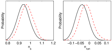
Figure 1: Marginalized distributions of the running spectral index slope parameters including (solid) and without (dashed) the WMAP temperature data at $\ell<5$.

In most parameter studies the scalar initial power spectrum is parameterized by a constant spectral index $n_{s}$ and an amplitude. Even with only two parameters defining the primordial power spectrum there are large degeneracies between these and the other cosmological parameters. For example larger baryon densities decrease the height of the CMB second acoustic peak thereby mimicking the effect of a red spectral tilt.

Using the WMAP (Hinshaw et al., 2003; Kogut et al., 2003) power spectrum results alone we find a tight marginalized constraint $n_{s}-30.4(\Omega_{b}h^{2}-0.025)=1.04\pm 0.02$ (68% confidence). However the orthogonal direction is very poorly constrained with $n_{s}+30.4(\Omega_{b}h^{2}-0.025)=1\pm 0.14$. The best fit model to the WMAP data (Spergel et al., 2003) with $n_{s}=0.97$ can be closely approximated by completely different models with $n_{s}>1.1$, higher reionization redshifts, rapid Hubble expansion and high power spectrum amplitude. On integrating out the value of $\Omega_{b}h^{2}$ the constraint on the spectral index weakens to $n_{s}=1.05\pm 0.08$. Similarly the amplitude of the primordial curvature fluctuations on $0.05{\rm Mpc}^{-1}$ scales is constrained by WMAP to be $A_{s}^{1/2}=(5.5\pm 0.8)\times 10^{-5}$, whereas the parameter combination $A_{s}^{1/2}e^{-\tau}=(4.3\pm 0.1)\times 10^{-5}$ is much more tightly constrained since it comes directly from the observed temperature anisotropy amplitude. To partially break these degeneracies the WMAP team adopt a prior on the reionization optical depth of $\tau<0.3$. By adding the 2dFGRS and additional CMB data at $\ell>800$ we find the parameter constraints which broadly agree with the analysis reported by the WMAP team (Spergel et al., 2003), see Fig. 5 below.

By adding a running spectral index we find the marginalized 1-sigma result $n_{\rm run}=-0.04\pm 0.03$ shown by the solid line in the right hand panel of Fig. 1, in rough agreement with the WMAP team. For the pivot scale used ($k_{s0}=0.05{\rm Mpc}^{-1}$) a red tilt is preferred (left hand panel of Fig. 1). As expected, the effect of adding $n_{\rm run}$ as a free parameter is to increase the uncertainties on the cosmological parameters but only within the original uncertainties.

We find that the evidence for running comes predominantly from the very largest scale multipoles. When we exclude $\ell<5$ multipoles from the WMAP temperature (TT) likelihood the running spectral index distribution shifts to becomes highly consistent with $n_{\rm run}=0$, as shown in Fig. 1 . The constraints on all cosmological parameters except for $n_{\rm s}$ and $n_{\rm run}$ are changed very little on removing the lowest multipoles. The running parameterization is therefore not ideally suited to the data: WMAP provides some evidence for low power on the very largest scales, but this is only crudely fit by using a running spectral index. The WMAP analysis relies on Lyman-$\alpha$ forest at wavenumbers greater than $k\sim 0.1{\rm Mpc}^{-1}$ to give evidence for more red tilt on small scales consistent with a running index, but the validity of this analysis is in serious doubt Seljak et al. (2003). We conclude that the marginal preference for a running spectral index from our CMB + 2dFGRS analysis is primarily driven by the first three CMB multipoles.

4 Power spectrum on the largest observable scales

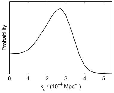
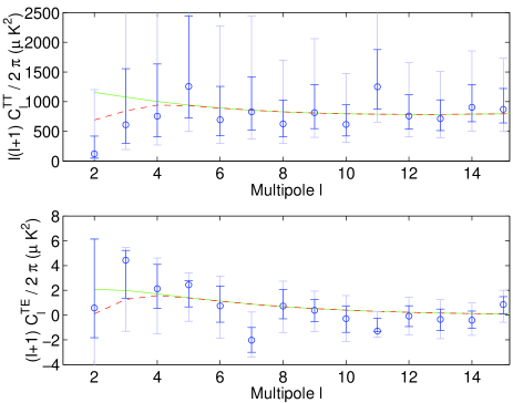
Figure 2: Top: Marginalized probability distribution of a large scale power cut-off parameter $k_{c}$ for which ${\cal P}_{\chi}(k<k_{c})=0$. Lower panels: a concordance model with $k_{c}=0$ (solid lines) and with $k_{c}=2.7\times 10^{-4}$ (dashed lines) compared to the WMAP data. Dark and light error bars show the 68 and 95 confidence limits on the theoretical value at each multipole (for the TE error bars we use the Gaussian contribution to the likelihood given the observed TT estimator, taking into account the correlation between the TT and TE estimators, assuming the WMAP best fit model for $C_{\ell}^{\rm TT}$ and $C_{\ell}^{\rm EE}$, where $(C_{\ell}^{\rm TE})^{2}<C_{\ell}^{\rm TT}C_{\ell}^{\rm EE}$).

The quadrupole and octopole estimators observed by WMAP are low compared to the other large scale multipoles. In a given model the low multipole estimators have a wide $\chi^{2}$-like distribution (which has the peak below the ensemble mean), so the low values could just be chance. However any model that predicts small values for the low multipoles would be favoured by the data, by a factor of up to about fourty, so this could be a hint that there is a sharp fall in power on the largest scales. Tegmark et al. (2003) find that the quadrupole and octopole appear to be aligned, perhaps indicative of some anisotropic effect on on very large spatial scales which would not be well modeled by a statistically isotropic power spectrum model. Here we assume that the alignment is a coincidence, and proceed to consider whether the shape of the initial power spectrum could help to explain the low large scale signal.

There is only a limited amount of information on the largest scales due to cosmic variance, so we cannot hope to fit many extra parameters. We choose to assume there is a sharp total cut-off in the primordial power on scales larger than $k=k_{c}$ (for a discussion of an exponential cut-off in closed models see Efstathiou (2003); see Contaldi et al. (2003) for possible motivation for a cut-off). As discussed in the previous section a constant spectral index is a good fit on smaller scales, so we parameterize the primordial spectrum as

$${\cal P}_{\chi}(k)=\left\{\begin{array}[]{c@{\qquad}l}0&k<k_{c}\\ A_{s}\left(\frac{k}{k_{s0}}\right)^{n_{s}-1}&k\geq k_{c}\,\,\,.\end{array}\right.$$ (4)

Marginalizing over the other parameters we find the constraint on $k_{c}$ shown in the upper panel of Fig. 2. We find a preference for a cut-off at $k_{c}=(2.7^{+0.5}_{-1.6})\times 10^{-4}{\rm Mpc}^{-1}$, a scale which can give a significantly lower quadrupole and octopole without significantly affecting the higher multipoles (lower panels of Fig. 2). However, according to this model a spectrum with no cut-off is not strongly excluded by the data. Our parameterization cannot achieve values for the quadrupole as low as observed because there is a significant Integrated-Sachs Wolfe contribution to the quadrupole from scales smaller than the cut. The best-fit cut-off model has a very similar probability to the best-fit running model, although the cut-off model is marginally preferred. The constraints on the cosmological parameters are virtually unaffected by adding this free cut-off scale.

A comparison with Spergel et al. (2003)’s assessment of the significance of the low CMB power at small multipoles is not straightforward because the statistical tests differ. A more detailed analysis of this important issue is required, but given the results of Fig. 2 it would seem premature to discard simple continuous power law models.

5 Power spectrum reconstruction in wavenumber bands

On smaller scales there is now a wealth of data available to constrain the primordial power spectrum in considerable generality. Here we choose to parameterize the spectrum in a number of bands, which has the advantage that it is free from any assumptions about the underlying model. This generality can in principle reveal unexpected features in the primordial power spectrum on scales comparable to (or larger than) the band width. The disadvantage is that there are a large number of free parameters so care is needed to obtain meaningful results.

The initial power spectrum is only indirectly constrained by the observational data. Since we do not model the biasing in the 2dFGRS galaxy power spectrum, the only direct constraint on the amplitude (as opposed to the shape) comes from the CMB anisotropy power spectra. On scales smaller than the horizon size at reionization ($\ell\sim 40$) the observed power in the CMB anisotropy scales as $e^{-2\tau}{\cal P}_{\chi}(k)$, depending on the optical depth to reionization $\tau$. We therefore parameterize the shape of the initial power spectrum by the value of $e^{-2\tau}{\cal P}_{\chi}(k)$ at a set of points, and linearly interpolate (in $k$) between the points. We then refer to the power at each point as the power in a ‘band’ at that wavenumber. Our parameters $b_{i}$ are defined by

$$e^{-2\tau}{\cal P}_{\chi}(k)=\left\{\begin{array}[]{c@{\qquad}l}\frac{(k_{i+1}-k)b_{i}+(k-k_{i})b_{i+1}}{k_{i+1}-k_{i}}&k_{i}<k<k_{i+1}\\ b_{n}&k>k_{n}\end{array}\right.$$ (5)

where the first line applies for $1\leq i\leq n-1$. We set the position of the first band to $k_{1}=0$ and that of the second band to $k_{2}=0.005{\rm Mpc}^{-1}$, so we only have two bands over the region where the data are effected by the modes which are super-horizon at reionization and hence do not scale simply with $e^{-2\tau}$. Subsequent band positions on smaller scales are logarithmically spaced with $k_{i+1}=1.275\,k_{i}$, where the constant is chosen such that $k_{16}=0.15{\rm Mpc}^{-1}$. We assume a flat prior on each of the $b_{i}$. This prior is equivalent to a flat prior on the underlying power spectrum $e^{2\tau}b_{i}$, together with a prior on the optical depth $P(\tau)\propto e^{-2n\tau}$. Constraints on quantities sensitive to $\tau$ depend strongly on the choice prior for large numbers of bands. This is one reason we reconstruct $b_{i}$, which are more directly constrained by the data and have the main dependence on $\tau$ taken out, rather than ${\cal P}_{\chi}(k)$ directly. Our choice of prior gives a posterior constraint on the optical depth similar to (but somewhat broader than) that with the simple spectral index parameterization.

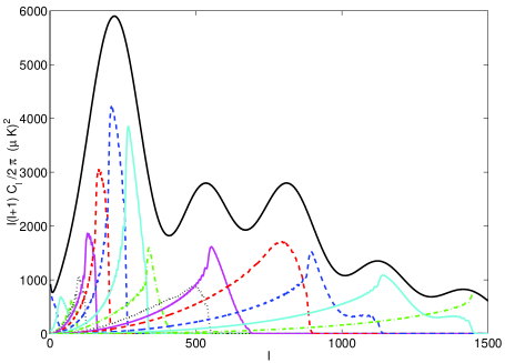
Figure 3: CMB power spectra for top hat primordial power spectra at the positions of the bins used for Fig. 4. The top line is the sum of all the lower lines, ie. the usual CMB power spectrum.

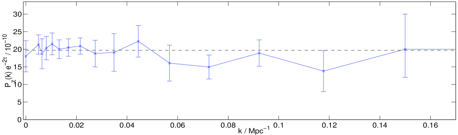
Figure 4: Reconstruction of the shape of the primordial power spectrum in 16 bands after marginalising over the Hubble constant, baryon and dark matter densities, and the redshift of reionization.

Fig. 3 shows the CMB temperature power spectra for top hat primordial power spectra which are zero except for the range $(k_{i-1}+k_{i})/2<k<(k_{i}+k_{i+1})/2$ (except for $i=1$ where $0<k<k_{2}/2$) for a concordance model. All the primordial power spectrum top hats have the same absolute height. The result illustrates the rough correspondence between the position of the bands we use and the CMB power spectrum peaks, showing that there is one band covering much of the large scales, and several bands over the first acoustic peak, with only one or two bands for each of the subsequent few peaks.

Our reconstruction of the shape of the initial power spectrum is shown in Fig. 4. The crosses and error bars show the peak and 68% upper and lower limits of the marginalized distributions. The probability distribution of all but the last band is close to Gaussian, although some bands are correlated at around the fifty per cent level. The maximum correlation is 80 per cent, which is a positive correlation between bands around the first acoustic peak of the CMB. We have checked that our constraints on the sub-horizon $b_{i}$ agree well with those obtained by fixing the optical depth to $\tau=0.17$ rather than marginalizing over it. The overall shape is consistent with a featureless scale invariant power spectrum, though perhaps an overall red tilt is discernible, bearing in mind the large error bar on the small scale point. We do not see the feature at $k\sim 0.015{\rm Mpc}^{-1}$ suggested by Mukherjee and Wang (2003b). Our reconstruction is complementary to that in Mukherjee and Wang (2003a) since our inter-band separation is one third of theirs. Also, we use linear interpolation instead of wavelets or top-hat bins, which makes the primordial power spectrum relatively smooth.

In Fig. 5 we investigate how robust the cosmological parameter estimates are to this general primordial power spectrum. Dashed lines show the cosmological parameter constraints assuming a power law primordial power spectrum, marginalising over $n_{s}$. Overlaid, the solid lines show the result after allowing freedom in the amplitudes of the 16 bands. The error contours are broader but remarkably show that it is still possible to recover interesting constraints on the cosmological parameters even if one allows the large amount of freedom in the primordial power spectrum shape.

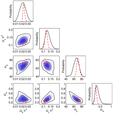
Figure 5: Constraints on cosmological parameter estimates after marginalising over the power spectrum amplitudes in 16 bands (solid lines), and for comparison equivalent results in the constant spectral index model (dashed lines). Contours enclose $68\%$ and $95\%$ of the probability.

It is important to emphasize that this method of power spectrum differs from earlier work such as that by Gawiser and Silk (1998) because the MCMC reconstruction properly accounts for the allowed ranges of all of the parameters defining the model.

6 Broken power spectrum

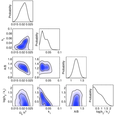
Figure 6: Marginalized constraints on the parameters of the broken power spectrum model and the correlations with the baryon density. The constraint on $\tau$ is changed relatively little on allowing the 16 bands, becoming $\tau=0.13\pm 0.07$

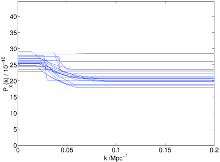
Figure 7: Primordial power spectra of random samples from the broken power spectra chains.

In this section we use a parameterization motivated by double inflation, previously explored by  Barriga et al. (2001). In this model

$${\cal P}_{\chi}(k)=\left\{\begin{array}[]{c@{\qquad}l}A&k<k_{1}\\ Ck^{\alpha-1}&k_{1}<k<k_{2}\\ B&k>k_{2}\,\,.\end{array}\right.$$ (6)

where $C$ and $\alpha$ are chosen such that the power spectrum is continuous. As in Barriga et al. (2001) we take flat priors on $k_{1}$, $A/B$ and $\log(k_{2}/k_{1})$ and we limit the parameter space to $0.01<k_{1}/{\rm Mpc^{-1}}<0.1$, $0.3<A/B<7.2$ and $0.01<\log(k_{2}/k_{1})<4$. In addition we impose a prior $k_{2}<0.1{\rm Mpc^{-1}}$ so that we explore a transition only in the region probed by the observational data.

In Fig. 6 we show the constraints on the model parameters after marginalising over four cosmological parameters. A conventional scale-invariant spectrum corresponds to $A/B=1$ and we can see that this possibility is very close to the 1$\sigma$ contours. Values of $A/B$ higher than unity are preferred, corresponding to a drop in the initial power spectrum on going from large to small scales. This is not surprising since the data favour red tilts, and in this parameterization a tilt is obtained by having a long transition between a higher flat spectrum on large scales and a lower flat spectrum on small scales. The distribution is slightly bimodal, with the first mode roughly corresponding to a wide transition straddling the first CMB acoustic peak and the second corresponding to a drop in power in the dip between the first and second peaks. The expected strong correlation between $A/B$ and the baryon density is clear. We find that removing the first three multipoles has no effect on the parameter constraints on this model.

We show in Fig. 7 the power spectra corresponding to 20 samples in the MCMC chain. There is considerable spread, but the transition, if any, occurs at around $k\sim 0.04{\rm Mpc^{-1}}$. This corresponds roughly to the scale at which the 2dFGRS data becomes statistically significant. Since the 2dFGRS data may disfavour a transition at higher wavenumber and the WMAP data would disfavour a transition at lower wavenumber then neither the amplitude or the scale of the break is likely to be of any physical significance.

The effect of adding these additional parameters on the estimates of cosmological parameters is small; the biggest effect is to widen the allowed range of $\Omega_{\rm b}h^{2}$ to include smaller values. This is due to the fact that a preferred position for any transition is between the first two acoustic CMB peaks, and it is also this ratio that determines the baryon density.

7 Conclusions

We have explored various parameterizations of the primordial power spectrum and found that in each case a simple scale invariant spectrum is an acceptable fit to the data. Some deviation towards a red tilt is preferred and there is a marginal indication of a cut-off in power on the largest observable scales. Significantly, even if the power spectrum is allowed to vary over a large number of wavenumber bands on sub-horizon scales the reconstructed spectrum is found to be featureless and close to scale invariant. In addition we have shown how the constraints on the other cosmological parameters are affected by the addition of this extra freedom in the primordial power spectrum shape: the error bars on cosmological parameters are significantly amplified but the resulting constraints are still strong and roughly similar to those before the recent WMAP results. The unexpectedly small power on superhorizon scales observed by WMAP, if real, provides marginal evidence for a drop in the primordial power spectrum on the largest observable scales.

References

- Albrecht and Steinhardt (1982) Albrecht A. and Steinhardt P. J., Phys. Rev. Lett. 48, 1220 (1982).
- Barriga et al. (2001) Barriga J., Gaztañaga E., Santos M. G., and Sarkar S., MNRAS 324, 977 (2001).
- Christensen et al. (2001) Christensen N., Meyer R., Knox L., and Luey B., Classical and Quantum Gravity 18, 2677 (2001).
- Contaldi et al. (2003) Contaldi C., Peloso M., Kofman L., and Linde A., (2003), astro-ph/0303636.
- Efstathiou (2003) Efstathiou G. (2003), astro-ph/0303127.
- Elgaroy et al. (2002) Elgaroy O., Gramann M., and Lahav O., MNRAS 333, 93 (2002).
- Gawiser and Silk (1998) Gawiser E. and Silk J., Science 280, 1405 (1998).
- Grainge et al. (2002) Grainge K. et al. (2002), astro-ph/0212495.
- Guth (1981) Guth A. H., PRD 23, 347 (1981).
- Hinshaw et al. (2003) Hinshaw M. et al. (2003), astro-ph/0302217.
- Kinney (2001) Kinney W. H., PRD 63, 43001 (2001).
- Kogut et al. (2003) Kogut et al. (2003), astro-ph/030221.
- Kuo et al. (2003) Kuo et al. (2003), astro-ph/0212289.
- Lewis and Bridle (2002) Lewis A. and Bridle S., PRD 66, 103511 (2002), astro-ph/0205436.
- Lewis et al. (2000) Lewis A., Challinor A., and Lasenby A., ApJ 538, 473 (2000).
- Linde (1982) Linde A. D., Phys. Lett. B108, 389 (1982).
- Linde (1990) Linde A. D., Particle physics and inflationary cosmology (Harwood Academic Publishers, Chur, Switzerland 1990, 1990).
- Lyth and Riotto (1999) Lyth D. H. and Riotto A. A., Physics Reports 314, 1 (1999).
- Mukherjee and Wang (2003a) Mukherjee P. and Wang Y. (2003a), astro-ph/0303211.
- Mukherjee and Wang (2003b) Mukherjee P. and Wang Y. (2003b), astro-ph/0301058.
- Mukherjee and Wang (2003c) Mukherjee P. and Wang Y. (2003c), astro-ph/0301562.
- Pearson et al. (2002) Pearson T. et al. (2002), astro-ph/0205388.
- Peiris et al. (2003) Peiris H. et al. (2003), astro-ph/0302225.
- Percival et al. (2002) Percival W. J. et al., MNRAS 337, 1068 (2002).
- Seljak et al. (2003) Seljak U., McDonald P., and Makarov A. (2003), astro-ph/0302571.
- Seljak and Zaldarriaga (1996) Seljak U. and Zaldarriaga M., ApJ 469, 437 (1996).
- Souradeep et al. (1998) Souradeep T., Bond J. R. , Knox L., Efstathiou G., and Turner M. S., in COSMO-97, Ambleside, England, September 1997, edited by L. Roszkowski (World Scientific, 1998), astro-ph/9802262.
- Spergel et al. (2003) Spergel D. et al. (2003), astro-ph/0302209.
- Steinhardt and Turok (2002) Steinhardt P. J. and Turok N., Science 296, 1436 (2002).
- Tegmark et al. (2003) Tegmark M., de Oliveira-Costa A., and Hamilton A. (2003), astro-ph/0302496.
- Tegmark and Zaldarriaga (2002) Tegmark M. and Zaldarriaga M., PRD 66, 103508 (2002).
- Verde et al. (2003) Verde L., et al. (2003), astro-ph/0302218.
- Wang and Mathews (2002) Wang Y. and Mathews G. J., ApJ 573, 1 (2002).
- Wang et al. (1999) Wang Y., Spergel D. N., and Strauss M. A., ApJ 510, 20 (1999).