A Quadruple Phase Strong Mgii Absorber at $z\sim 0.9902$ Toward PG $1634+706$

Abstract

The $z=0.9902$ system along the quasar PG $1634+706$ line of sight is a strong Mgii absorber ($W_{r}(2796)>0.3$ Å) with only weak Civ absorption (it is “Civ–deficient”). To study this system, we used high–resolution spectra from both the Hubble Space Telescope (HST)/Space Telescope Imaging Spectrograph (STIS) and the Keck I telescope/High Resolution Echelle Spectrometer (HIRES). The STIS spectrum has a resolution of $R=30,000$ and covers key transitions, such as Siii, Cii, Siiii, Ciii, Siiv, and Civ. The HIRES spectrum, with a resolution of $R=45,000$, covers the Mgi, Mgii and Feii transitions. Assuming a Haardt and Madau extragalactic background spectrum, we modeled the system with a combination of photoionization and collisional ionization. Based on a comparison of synthetic spectra to the data profiles, we infer the existence of the following four phases of gas:

i) Seven Mgii clouds have sizes of $1$–$1000$ pc and densities of $0.002$–$0.1$ cm^-3, with a gradual decrease in density from blue to red. The Mgii phase gives rise to most of the Civ absorption and resembles the warm, ionized inter-cloud medium of the Milky Way;

ii) Instead of arising in the same phase as Mgii, Mgi is produced in separate, narrow components with $b\sim 0.75$ km s^-1. These small Mgi pockets ($\sim 100$ AU) could represent a denser phase ($\sim 200$ cm^-3) of the interstellar medium (ISM), analogous to the small–scale structure observed in the Milky Way ISM;

iii) A “broad phase” with a Doppler parameter, $b\sim 60$ km s^-1, is required to consistently fit Ly$\alpha$, Ly$\beta$, and the higher–order Lyman–series lines. A low metallicity ($\log Z\lesssim-2$) for this phase could explain why the system is “Civ–deficient”, and also why Nv and Ovi are not detected. This phase may be a galactic halo or it could represent a diffuse medium in an early–type galaxy;

iv) The strong absorption in Siiv relative to Civ could be produced in an extra, collisionally ionized phase with a temperature of $T\sim 60,000$ K. The collisional phase could exist in cooling layers that are shock–heated by supernovae–related processes.

1 Introduction

Quasar absorption lines provide a unique and intriguing way to determine the kinematics, chemical composition, and ionization state of gas in intervening galaxies. For most galaxies, a multi–phase interstellar medium (ISM) (i.e. a medium with different densities and temperatures) is likely to exist (McKee & Ostriker, 1977; Giroux, Sutherland, & Shull, 1994). Thus, it follows that any random line of sight passing through a galaxy is likely to encounter several phases of gas.

Strong Mgii absorbers ($W_{r}(2796)>0.3$ Å) are almost always found within an impact parameter of $35h^{-1}$ kpc of a luminous galaxy ($>0.05L^{*}$), where $L^{*}$ is the Schechter luminosity (Bergeron & Boissé, 1991; Bergeron et al., 1992; Le Brun et al., 1993; Steidel, Dickinson, & Persson, 1994; Steidel, 1995; Steidel et al., 1997). In addition, the strong Civ absorption that is characteristic of most such absorbers is thought (Churchill et al., 1999, 2000) to arise in a corona similar to that surrounding the Milky Way disk (Savage et al., 1997).

We study the $z=0.9902$ system along the line of sight to the quasar PG $1634+706$ ($z_{em}=1.335$). This system is a strong Mgii absorber with at least five blended components and with a deficiency of Civ relative to other systems with similar $W_{r}({\hbox{{\rm Mg}\kern 1.00006pt{\sc ii}}})$ (Churchill et al., 2000). In a previous study, Charlton et al. (2000) derived constraints on the physical properties of the system, based upon the combination of low–resolution data from the Faint Object Spectrograph (FOS) on–board the Hubble Space Telescope (HST) and high–resolution data from the High Resolution Echelle Spectrometer (HIRES) on the Keck I telescope. At that time, only low–resolution data were available for many key transitions, including low–ionization tracers (Siii and Cii), high–ionization tracers (Siiv and Civ), and the Lyman–series lines. However, the HIRES profiles of Mgi, Mgii, and Feii were used to form a template that was applied to model the low–resolution data.

Based on the FOS and HIRES data, Charlton et al. (2000) came to the following conclusions: (1) The metallicity (expressed in the solar units) of the Mgii phase would be low ($-1.5\lesssim\log Z\lesssim-1$) if it was to produce a full Lyman limit break; (2) A broad component ($40\lesssim b({\rm H})\lesssim 80$ km s^-1) was needed to fit the Ly$\alpha$ profile; (3) An additional broad component also appeared to be needed to produce Civ; (4) Siiv could not fully arise in the inferred low– or high–ionization phases, which suggested the existence of a blend or an additional component.

However, some important issues still remained unresolved: (1) whether the Mgi could be produced in the same clouds as Mgii; (2) whether the ionization conditions vary across the profiles; (3) whether Civ is produced by a single, broad phase or by several separate, narrower clouds; and (4) whether Siiv is affected by a blend and, if not, how is it produced?

The first issue is important because Mgi is under–produced by the Mgii phase in many strong Mgii absorption systems (Churchill, 1997; Churchill, Vogt, & Charlton, 2002). In addition, Mgi absorption is often very strong in the environment where damped Ly$\alpha$ absorbers (DLAs) arise and therefore could be used to trace the origin of the strongest Hi absorption. A resolution to the Mgi/Mgii issue in the case of the $z=0.9902$ Mgii system could serve as a basis for solving these more general problems.

The third issue is of particular interest because this system is Civ–deficient (Churchill et al., 2000). Most strong Mgii absorbers have comparable strong Civ absorption, which is likely to arise in a corona similar to that surrounding the Milky Way. Although Civ is detected in the low–resolution FOS spectrum, it is relatively weak. Therefore, the additional component suggested by Charlton et al. (2000) may not be analogous to a corona. The Civ profiles could be resolved to determine whether the “corona phase” is absent, or just weak in Civ. Either low metallicity or high–ionization conditions could lead to weak Civ absorption from a corona.

With the release of grating E230M spectra from the Space Telescope Imaging Spectrograph (STIS) on–board the HST, we now have high–resolution coverage of the Lyman series, Siii, Cii, Siiii, Ciii, Siiv, and Civ transitions. In this paper, we present the results from photo–/collisional ionization modeling of the $z\simeq 0.9902$ Mgii system. Combining the newer data with those on the Mgi, Mgii, and Feii from Keck/HIRES, we determine the minimum number of phases required to produce the observed absorption in the many detected chemical transitions. For each phase, we place constraints on physical properties such as densities, temperatures, and sizes of the various environments that give rise to the absorption features displayed in the observed spectral profiles.

In § 2, we briefly describe the data that we use to constrain our models. A summary of our modeling techniques is presented in § 3 and our major results are outlined in § 4. Finally, in § 5, we summarize and give a physical interpretation of the system.

2 Data and Analysis

2.1 Keck/HIRES

The optical part of the spectrum (with Mgi 2853, Mgii 2796, Mgii 2803 and Feii 2600 covered between 3723 Å and 6186  Å) was obtained from the HIRES on the Keck I telescope on July 4 and 5, 1995 (Vogt et al., 1995). This spectrum has a resolution of $R=45,000$ (FWHM $\sim 6.6$ km s^-1) and a signal–to–noise ratio of $\sim 50$ per three–pixel resolution element (Charlton et al., 2000).

The HIRES spectrum was reduced with the IRAF APEXTRACT package for echelle data and was extracted using the optimal extraction routine of Horne (1986) and Marsh (1989). The wavelengths were calibrated to vacuum using the IRAF task ECIDENTIFY, and shifted to heliocentric velocities. Continuum fitting was based on the formalism of Sembach & Savage (1992).

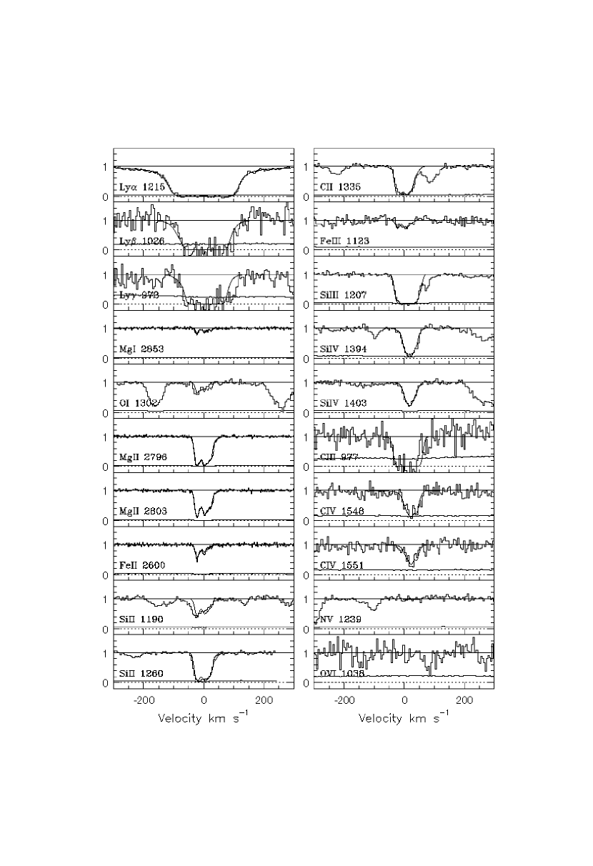
Figure 1: The normalized STIS and HIRES profiles of various key transitions are displayed in velocity space. The velocity zero–point is at $z=0.9902$. The solid curve just above zero represents the $1{\sigma}$ error bar. The curve superimposed on the data is a synthetic spectrum for one of the best models we have considered (summarized in Table 1). The Mgi, Mgii, and Feii profiles were observed with Keck/HIRES, and all the others with HST/STIS.

Voigt profiles were used to simultaneously fit Mgi, Mgii, and Feii, with free parameters redshift, column density and Doppler parameter, $b$, for each component. The program MINFIT (Churchill, 1997), using a $\chi^{2}$ formalism, found the minimum number of components required to fit the system. The Mgi 2853, Mgii $\lambda\lambda 2796,2803$ and Feii 2600 transitions, covered by HIRES, are shown in velocity space in Figure 1. Other Feii transitions were also covered, but Feii 2600 has the highest signal–to–noise.

The fitting procedure was summarized in Churchill & Vogt (2001), and described in detail in Churchill (1997). Components are dropped from the fit unless retaining them produces a $\chi^{2}$ value that is significantly better ($97$ % by the F–test). Errors in redshifts, column densities, and Doppler parameters were determined, using the diagonal elements of the covariance matrix, determined from the curvature matrix. Components were rejected if their total fractional errors exceeded $1.5$.

2.2 HST/FOS

Before the release of the STIS data, low–resolution UV spectra were obtained using the G190H and G270H gratings of HST/FOS. These spectra were presented in Impey et al. (1996) and Bahcall et al. (1996). Since the higher–resolution STIS spectrum covers most of the key transitions for the $z=0.9902$ system, we only used the FOS spectra to study the Lyman limit break at $1830$ Å, which implies the neutral hydrogen column density $\log N({\hbox{{\rm H}\kern 1.00006pt{\sc i}}})\gtrsim 18$. The data reduction, wavelength calibration, fluxing, and continuum fitting of the FOS spectra were performed as part of the QSO Absorption Line Key Project (Bahcall et al., 1996).

2.3 HST/STIS

Two high–resolution ($R=30,000$) datasets, with different wavelength coverage, were obtained with HST/STIS and retrieved from the HST data archive. The E230M spectrum, obtained by S. Burles (May and June 2000), has a wavelength coverage of $1865$ Å to $2673$ Å, and a total exposure time of $29,000$ seconds. The E230M spectrum, provided by B. T. Jannuzi (June 2000), has a wavelength coverage of $2303$ Å to $3111$ Å, and a total exposure time of $26,435$ seconds. The Lyman series, Siii, Cii, Siiii, Ciii, Siiv, and Civ are all covered by the E230M STIS spectra. A G230M spectrum, covering 1830 Å to 1870 Å, was also obtained by S. Burles (May 2000), but it did not cover any key transitions for our analysis of the system.

The STIS spectra were reduced using the standard pipeline (Brown et al., 2002). The extracted spectra were averaged between different exposures and the continuum fitting was performed with standard IRAF tasks (Churchill & Vogt, 2001).

The spectra of various transitions are shown in Figure 1. Ly$\gamma$ is apparently blended with another feature, based on its asymmetry relative to the other Lyman–series transitions. Ly$\delta$ is not shown due to its noisy spectrum and its contamination by a blend. Siii 1190 is blended with Nv 1243 from the $z=0.9056$ system. Cii 1335 is contaminated by Siiv 1394 from the $z=0.9056$ system, but based on Siiv 1403, the contribution from Siiv 1394 would be negligible. A relatively strong, unidentified feature is apparent to the red of the Cii 1335 profile. Siiii 1207 is blended with Siii 1260 from the $z=0.9056$ system. Only Nv 1239 is shown because no absorption is detected in either of the Nv $\lambda\lambda 1238,1242$ profiles and Nv 1239 is the stronger of the two. Ovi 1032 is not shown. It is clearly inconsistent with the undetected Ovi 1038.

3 Methods for Modeling

The goal of the present study was to determine the physical conditions under which the spectra shown in Figure 1 were produced. To begin, we applied a Voigt profile fit to the Mgii transitions to determine the locations, column densities, and Doppler parameters of the components required to reproduce the observed absorption. We assumed that each one of these components was produced by an individual “cloud” and we modeled each one of these clouds with the photoionization code Cloudy, version 90.4 (Ferland 1996).

The clouds were assumed to be constant–density, plane–parallel slabs in photoionization equilibrium. They were ionized by a $z=1$ Haardt and Madau (1996) extragalactic background spectrum normalizing with an ionizing photon density of $\log n_{\gamma}=-5.2$. Alternative input spectra were also briefly explored, as discussed in § 4.5. To simulate these clouds, the required input parameters were: i) the column density of Mgii, $N({\hbox{{\rm Mg}\kern 1.00006pt{\sc ii}}})$, ii) the metallicity, $Z$ (expressed in the units of the solar value), iii) the ionization parameter, $U$ (defined as the ratio of the number density of photons capable of ionizing hydrogen, $n_{\gamma}$, to the number density of hydrogen, $n_{H}$), and iv) the abundance pattern. The column density of Mgii was obtained from the Voigt profile fit. Both the metallicity and the ionization parameter were chosen from a range reasonable for interstellar and intergalactic clouds (i.e. $-3\lesssim\log Z\lesssim 0$ and $-5\lesssim\log U\lesssim 0$), with the initial assumption of a solar abundance pattern. If a simultaneous fit to all transitions was not possible with solar abundances, alternatives were explored.

Once the input parameters were specified, we ran Cloudy to optimize on the column density of a selected species, such as Mgii. During the run, Cloudy used an initial guess of $N({\hbox{{\rm H}\kern 1.00006pt{\sc i}}})$ and calculated the corresponding $N({\hbox{{\rm Mg}\kern 1.00006pt{\sc ii}}})$. The output $N({\hbox{{\rm Mg}\kern 1.00006pt{\sc ii}}})$ was compared to the value measured from the Voigt profile fit, and the value of $N({\hbox{{\rm H}\kern 1.00006pt{\sc i}}})$ was adjusted accordingly for the next iteration. This process was repeated until the difference between the output $N({\hbox{{\rm Mg}\kern 1.00006pt{\sc ii}}})$ and the designated one was negligible.

Upon the completion of the final iteration, the following parameters were retrieved for the resulting cloud: the column density of every species with spectral coverage, the size of the cloud, and the temperature. The temperature was used to calculate the thermal component of the Doppler parameter of each ion, according to $b_{therm}^{2}=2kT/m$, where $m$ is the atomic weight of the ion. The turbulent component of $b$, which is due to the bulk motion of the gas and is the same for all the ions, was calculated from the measured $b({\rm Mg})$ using $b_{turb}^{2}=b^{2}({\rm Mg})-b_{therm}^{2}({\rm Mg})$. Combining the turbulent and thermal components, we obtained the Doppler parameter of all other individual ions.

Cloudy was run for all five Mgii clouds, each time calculating $N$ and $b$ for each species. A “pure” spectrum was then produced for each transition from the $N$ and $b$ of all five components. Then, we generated a synthetic spectrum by convolving the “pure” spectrum with the instrumental spread function. Finally, the synthetic spectrum was superimposed on the observed one for comparison.

We experimented with various metallicities and ionization parameters and attempted to obtain a synthetic spectrum that displayed minimal discrepancy with the observed one. A visual comparison of goodness of fit was used to reject models, as illustrated in Charlton et al. (2000) and Rigby et al. (2002). This was adequate to confidently constrain parameters to a relatively narrow range within the very large parameter space. The $\log U$ and $\log Z$ values given below are accurate to about $0.1$ dex. We considered using a quantitative $\chi^{2}$ approach, but found it to be impractical because a single pixel or group of pixels for a particular transition often dominated the assessment.

We encountered several issues that were unresolvable using a single phase of gas: Mgi was under–produced for any choice of $U$; the shape of the Ly$\alpha$ profile could not be fit; the velocity centroids of Siiv and Civ were offset from that of Mgii; and the Siiv and Civ transitions could not be fit simultaneously. Additional clouds were included in the Mgii phase to account for the offset Siiv and Civ absorption. The resolution of the other three issues requires the inclusion of independent phases: A colder, denser phase is needed to produce the observed absorption in Mgi. A broad, low–metallicity component is needed to account for the shape of the Ly$\alpha$ profile. Finally, a collisionally ionized phase is needed to fit Siiv without over–producing Civ. Each of these phases will be explained in detail in § 4.

4 Results

Here we present constraints on each of the four phases required to fit the $z=0.9902$ system, beginning with the lowest–ionization phase. Table 1 provides a summary of the cloud properties for all four phases in a plausible model that satisfies all constraints.

4.1 Mgi Phase

The five Mgii clouds from the original Voigt profile fit could not produce the observed equivalent width of Mgi, regardless of the choice of ionization parameter. The ratio $N({\hbox{{\rm Mg}\kern 1.00006pt{\sc i}}})$/$N({\hbox{{\rm Mg}\kern 1.00006pt{\sc ii}}})$ is nearly constant at $\simeq 0.01$ over a large range of ionization parameters, $U$, and for the range of metallicity appropriate for this system.

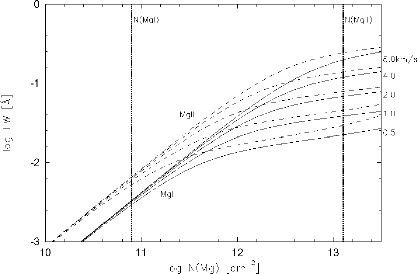
Figure 2: Equivalent width is plotted vs. column density, both on logarithmic scales. The dashed lines represent curves of growth for Mgii 2796, while the solid ones represent Mgi 2853 curves of growth. For both transitions, a set of Doppler parameters, $b=8.0,4.0,2.0,1.0$ and $0.5$ km s^-1, are indicated. Dotted lines represent typical $N({\hbox{{\rm Mg}\kern 1.00006pt{\sc ii}}})$ and $N({\hbox{{\rm Mg}\kern 1.00006pt{\sc i}}})$ values, i.e. those for the cloud at $-22$ km s^-1. From the curve it is shown that for our system Mgi is typically on the linear part of the curve of growth, while Mgii is on the flat part.

In order to obtain the observed equivalent width ratio $W_{r}(2853)/W_{r}(2796)$, a difference in the curve of growth between the two transitions was used, as shown in Figure 2. In general, when an absorption profile is unsaturated, its equivalent width, $W_{r}$, increases linearly with its column density, $N$ (i.e. on the linear part of curve of growth). However, when the absorption becomes saturated, $W_{r}$ stays almost constant with $N$, at a value that depends only on Doppler parameter, $b$ (i.e. on the flat part of curve of growth). In Figure 2, our typical $N({\hbox{{\rm Mg}\kern 1.00006pt{\sc ii}}})$ is on the flat part of the curve of growth, while $N({\hbox{{\rm Mg}\kern 1.00006pt{\sc i}}})$ is on the linear part. Thus, we could produce a larger $W_{r}(2853)/W_{r}(2796)$ using a smaller $b$, in a “Mgi phase”.

A unique Voigt profile fit to Mgi could not be obtained. We assumed five clouds at the same velocities as the broader Mgii cloud components, with a constant Doppler parameter and a constant ionization parameter. The Doppler parameter is constrained to be $b\lesssim 1$ km s^-1, in order that Mgii is not over–produced by the combination of this Mgi phase and the Mgii cloud phase (see § 4.2). However, the ionization parameter has to be $\log U\lesssim-8$ for $b=1$ km s^-1, in order that Oi is not over–produced. Alternatively, $\log U\lesssim-7.5$ if $b=0.75$ km s^-1 (Oi is on the flat part of the curve of growth). Column densities for a sample model with $b({\rm Mg})=0.75$ km s^-1 and $\log U=-7.5$ are listed in Table 1. With $b({\rm Mg})=0.75$ km s^-1, the temperature is constrained to be lower than $800$ K. Cloudy yields an effective temperature close to this value for the clouds in our sample model. An ionization parameter of $\log U=-7.5$ corresponds to a cloud density of $n(H)\simeq 200$ cm^-3. The cloud sizes are quite small, ranging from $60$–$160$ AU.

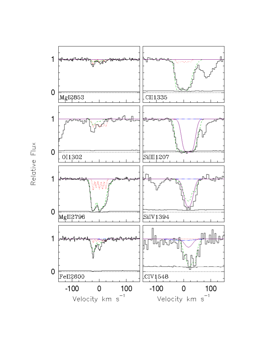
Figure 3: Various key metal transitions are plotted in velocity space. The STIS and HIRES data are histograms, with model curves superimposed. The dotted curves represent the Mgi clouds. The dashed curves show the contribution from the Mgii phase. The dashed–dotted curves represent the broad Hi phase. The solid curves show the contribution from the collisional component.

If the $b$ parameter is small, the Mgi phase will have trivial contribution to the overall equivalent width of any high–ionization metal transition. In Figure 3, the dotted lines represent the contribution from the Mgi phase for the model listed in Table 1. The contribution to Mgii is negligible, therefore Mgii has to be entirely produced by the Mgii cloud phase (see § 4.2).

Assuming the five Mgi clouds have the same metallicity, the metallicity of this phase is constrained to be $\log Z\gtrsim-0.8$, by the Ly$\alpha$ profile. At $\log Z=-0.8$, the Hi column densities of the five Mgi clouds are in the range of $17.3\lesssim\log N({\hbox{{\rm H}\kern 1.00006pt{\sc i}}})\lesssim 17.7$, as listed in Table 1, yielding an effective total of $\log N({\hbox{{\rm H}\kern 1.00006pt{\sc i}}})\simeq 18.1$. Thus, at this metallicity, the Mgi phase will give rise to the full Lyman limit break detected in the FOS spectrum, which requires $\log N({\hbox{{\rm H}\kern 1.00006pt{\sc i}}})\gtrsim 18$.

4.2 Mgii Phase

The column densities and $b$ parameters of the five Mgii clouds were obtained from a Voigt profile fit to the residuals in Mgii unaccounted for by the Mgi phase. The five clouds in this phase have considerably larger $b$ parameters ($6\lesssim b({\rm Mg})\lesssim 15$ km s^-1) than the Mgi clouds, as listed in Table 1.

With the detection of strong Feii in clouds ${\hbox{{\rm Mg}\kern 1.00006pt{\sc ii}}}_{1}$, ${\hbox{{\rm Mg}\kern 1.00006pt{\sc ii}}}_{2}$, and ${\hbox{{\rm Mg}\kern 1.00006pt{\sc ii}}}_{3}$, the ionization parameters of these clouds are constrained by $N({\hbox{{\rm Fe}\kern 1.00006pt{\sc ii}}})$/$N({\hbox{{\rm Mg}\kern 1.00006pt{\sc ii}}})$. The remaining two clouds (${\hbox{{\rm Mg}\kern 1.00006pt{\sc ii}}}_{4}$ and ${\hbox{{\rm Mg}\kern 1.00006pt{\sc ii}}}_{5}$) must have higher ionization parameters, since Feii is very weak. Siiv was used to determine their ionization states, with the assumption that the Siiv transitions arise in the same phase as Mgii. Thus, the five clouds have ionization parameters of $\log U\simeq-3.7$, $-4.0$, $-3.5$, $-3.0$, and $-2.5$, respectively, as listed in Table 1.

The Siiv and Civ profiles are not aligned with the bulk of the absorption seen in Mgi, Mgii, and the other low–ionization transitions. Thus, additional offset clouds with higher ionization parameters are needed. A Voigt profile fit to Siiv yielded two additional clouds (${\hbox{{\rm Mg}\kern 1.00006pt{\sc ii}}}_{6}$ and ${\hbox{{\rm Mg}\kern 1.00006pt{\sc ii}}}_{7}$) at $v\sim 42~{}$ and $v\sim 55~{}$km s^-1, respectively. Again, column densities and $b$ parameters of these two clouds are listed in Table 1. Ionization parameters are constrained to be $\log U\simeq-2.5$ and $-2.7$, by $N({\hbox{{\rm Si}\kern 1.00006pt{\sc iv}}})$/$N({\hbox{{\rm C}\kern 1.00006pt{\sc iv}}})$. This is also consistent with the weak absorption displayed in the red wings of the Mgii and Siii profiles.

A wide range of ionization states ($-4.0\lesssim\log U\lesssim-2.5$) is displayed in this Mgii phase, with a tendency for increase in ionization stage from blue to red in the spectrum. Therefore, most of the absorption in both low–ionization transitions, such as Mgii, Feii, Siii, and Cii, and high–ionization transitions, such as Siiii, Ciii, and Civ, is produced in this phase, as shown in Figure 3. However, the substantial under–production of Siiv suggests the existence of an extra component, as discussed in § 4.4.

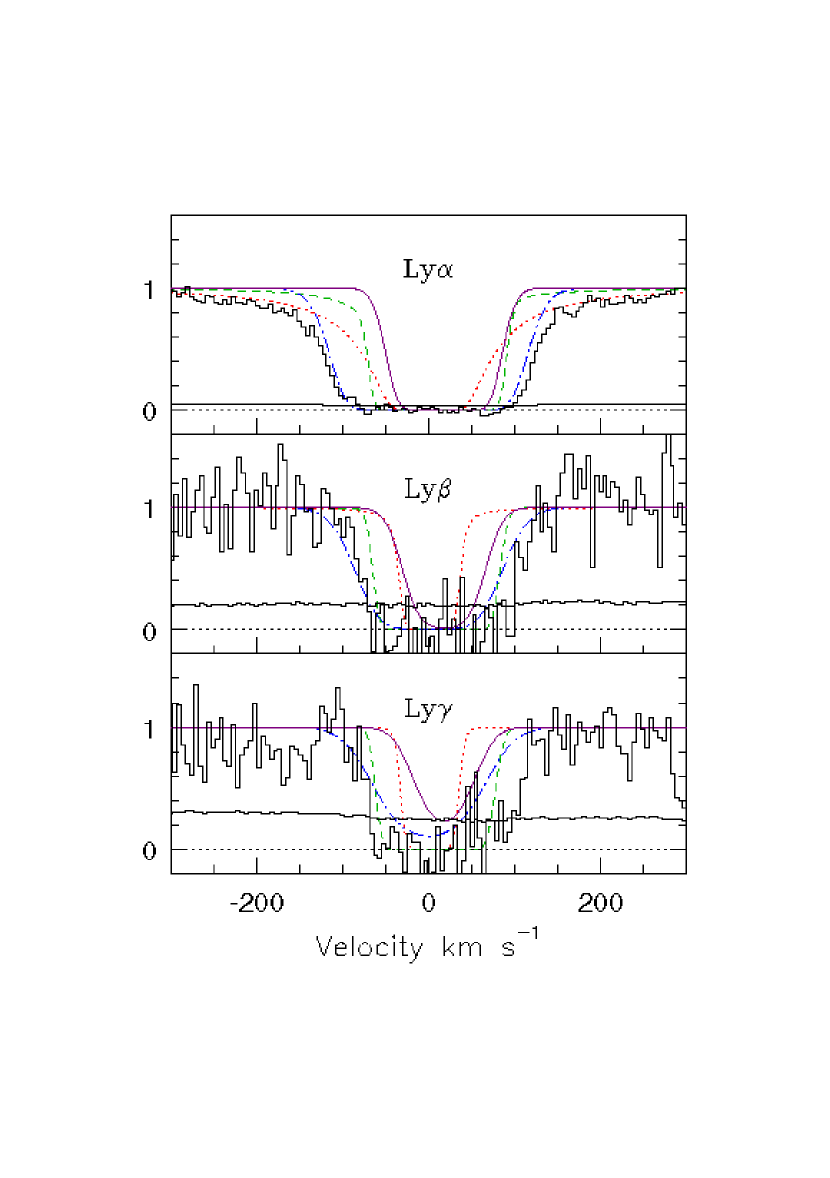
Figure 4: The Ly$\alpha$, Ly$\beta$, and Ly$\gamma$ profiles are displayed in velocity space. The solid histograms represent the STIS data. Other curves show the results for our “best model” (listed in Table 1). The model curves represent different phases as indicated in the caption of Figure 3.

Assuming that all seven clouds in the Mgii phase have the same metallicity, the metallicity is constrained to be $\log Z\gtrsim-0.65$ by the Lyman series. However, even at the lower limit of $\log Z=-0.65$, with $14.9\lesssim\log N({\hbox{{\rm H}\kern 1.00006pt{\sc i}}})\lesssim 17.1$, the Mgii phase contributes insignificantly to the observed full Lyman limit break. Alternatively, if the Mgi and Mgii phases are assumed to have the same metallicities, a metallicity of $\log Z\simeq-0.8$ is required by the Ly$\alpha$ profile (Figure 4). As mentioned in § 4.1, at this metallicity the five Mgi clouds will give rise to the observed full Lyman limit break (see Table 1).

4.3 Broad Hi Phase

The Ly$\alpha$ profile is too broad to be fully produced by the Mgi and Mgii clouds, as is shown in Figure 4. However, if the metallicity was decreased to give rise to more Ly$\alpha$, the narrower Ly$\gamma$ would be over–produced. The curve of growth of the Lyman–series lines (Churchill & Charlton, 1999) allows for a centered, broad component that can resolve this dilemma (i.e. it accounts for the broader, deeper Ly$\alpha$ profile, as well as the wing structure in Ly$\beta$, without over–producing the narrower Ly$\gamma$ profile.)

A Voigt profile fit to Ly$\alpha$ yielded the column density and $b$ parameter of the broad phase. If $b({\rm H})\gtrsim 70$ km s^-1 and $N({\hbox{{\rm H}\kern 1.00006pt{\sc i}}})\lesssim 10^{15}~{}$cm^-2, we can produce the saturated absorption from $-100$ to $+120$ km s^-1, but the wings will be over–produced; if $b({\rm H})\lesssim 50$ km s^-1 and $N({\hbox{{\rm H}\kern 1.00006pt{\sc i}}})\gtrsim 10^{16}~{}$cm^-2, we can produce the range of the saturated absorption, but the wings will be under–produced. The best fit was found to be with $N({\hbox{{\rm H}\kern 1.00006pt{\sc i}}})\sim 10^{15.5}~{}$cm^-2 and $b({\rm H})\sim 58$ km s^-1.

In principle, the broad component could be either photoionized or collisionally ionized. In both cases, the metallicity is constrained so as not to over–produce any of the high–ionization transitions (i.e. Civ, Nv and Ovi). The Nv and Ovi are not detected, and Civ is fully produced in the Mgii phase (as required by the structure appearing in the Civ profiles.).

For photoionization, an upper limit of $\log Z\lesssim-2$ is placed on the metallicity, regardless of the choice of ionization parameter. Otherwise, either low– or high–ionization transitions would be over–produced. If the metallicity is $\log Z\lesssim-2.5$, there will be no constraint on the ionization parameter from the metal transitions. None of them is significantly produced at such a low metallicity. However, a rough upper limit of $\log U\lesssim-1$ can be estimated by the requirement of a reasonable cloud size (less than several hundred kpcs). A good fit for this phase was obtained for a model with a metallicity of $\log Z\simeq-2.5$ and an ionization parameter of $\log U\simeq-1.5$, as listed in Table 1. This model gives a cloud $\sim 60$ kpc in size. The fit to the Lyman series is shown by the dashed–dotted curve in Figure 4.

For collisional ionization with pure thermal broadening (i.e. no bulk motion), the temperature would be $T\sim 10^{5.3}$ K, using $b^{2}=2kT$/$m$ for Hi. At this temperature, the metallicity has to be exceptionally low, $\log Z\lesssim-3.5$, in order not to over–produce the high–ionization transitions. If, instead, bulk motion contributes, the $b$ parameter will be larger for each metal species than the one given by pure thermal scaling of $b({\rm H})$. For example, as the temperature decreases from $T\sim 10^{5.3}$ K, $N({\hbox{{\rm C}\kern 1.00006pt{\sc iv}}})$ increases towards a peak at $T\sim 10^{5.0}$ K. This, together with a larger $b({\rm C})$, gives a larger Civ equivalent width when bulk motion is involved. In order not to over–produce Civ, the metallicity has to be even lower than the pure thermal case. A metallicity as low as $\log Z\sim-3.5$ is unlikely. Therefore, collisional ionization is ruled out for this phase. The broad Hi absorption is more likely to arise in a photoionized cloud, but even then the metallicity is constrained to be quite low ($\log Z\lesssim-2$).

4.4 Collisional Ionization Phase

The broad, smooth absorption profiles in the Siiv transitions are not consistent with the structure apparent in the Civ profiles. Because Siiv is offset relative to Ly$\alpha$, it also cannot be produced by the centered, broad Hi phase. The need to produce Siiv without contributing a substantial amount of absorption to other transitions suggests the existence of a collisionally ionized phase. A Voigt profile fit to the residuals in Siiv yielded a component at $v\sim 17~{}$km s^-1, with $N({\hbox{{\rm Si}\kern 1.00006pt{\sc iv}}})\sim 10^{13.5}~{}$cm^-2 and $b({\rm Si})\sim 17$ km s^-1. However, for collisional ionization, Siiv peaks at $\log T\sim 4.8$ (Sutherland & Dopita, 1993), which corresponds to $b_{therm}\sim 6$ km s^-1. Therefore, bulk motion must also contribute to the overall velocity dispersion. The temperature range was found to be $10^{4.7}\lesssim T\lesssim 10^{4.9}$ K, in order not to over–produce the transitions of higher– and lower–ionization stages. The metallicity of this phase could be set to the same value as the Mgi and Mgii phases, $\log Z\simeq-0.8$, but it is not well constrained. A lower limit of $\log Z\gtrsim-3$ is placed by the the Lyman–series lines.

4.5 Effects of Assumed Input Spectrum

For all the previous results, we have used the $z=1$ Haardt and Madau extragalactic background radiation (EBR) spectrum (Haardt & Madau, 1996) as the only source of ionizing photons. Here we consider the likelihood of additional stellar contributions and consider the effect of such alternative spectra in a couple of extreme examples.

At redshift $z\sim 1$ the extragalactic background radiation is more likely to dominate stellar contributions than it is at other redshifts. At lower redshifts, the amplitude of the Haardt and Madau extragalactic background is lower (by a factor of seven at $z=0$ (Haardt & Madau, 1996)). At much higher redshifts, starbursts are common and the amplitude of the EBR from quasars has levelled off.

Unfortunately, in the case of the PG $1634+459$ line of sight, we have no information about the colors or morphologies of the host galaxies. Therefore, we cannot rule out a starburst host for the $z=0.9902$ absorber. Only an extreme starburst would affect the results, and only within $\sim 6$ kpc of the center of such a galaxy would the stellar contribution strongly dominate the EBR ($1$% of the photon flux of $10^{54}~{}{\rm s}^{-1}$ would escape the burst region (Hurwitz, Jelinsky, & Dixon, 1997)). We would expect the absorption from the central region of a starburst to be stronger than it is for this $z=0.9902$ system (Bond et al., 2001). Furthermore, we would expect to pass through some layers of highly ionized gas, and this absorber is weak in Civ and undetected in Nv and Ovi. Therefore, a strong starburst host galaxy is unlikely, but we still consider here the effect of a couple of modified spectra.

Many different spectral shapes would be possible once we allow a stellar contribution and it is unrealistic to consider them all, so we choose two extreme cases: 1) a $0.01$ Gyr instantaneous burst, which is characterized by the edges of Hi, Hei, and Heii; and 2) a $0.1$ Gyr instantaneous burst with an extreme Hi edge, but with a relatively flat spectrum above that edge, similar to the Haardt and Madau shape. Both stellar spectra, assuming solar metallicity and a Salpeter IMF, were taken from Bruzual & Charlot (1993). We have run models with the burst contribution set to ten times that of the EBR, at $1$ Rydberg. We begin with the model in Table 1 and consider how the addition of the burst would affect our conclusions. In a more realistic model, however, the spectral shape would be a function of position, with the EBR likely to be dominant at some locations, but the solution to that case would be in between the extreme starburst models and a pure Haardt and Madau model.

Stellar contributions from a non-burst model are more likely to dominate the EBR at energies less than $1$ Rydberg. This could affect the ionization balance between the neutral and singly ionized transitions. Because of its extreme Lyman limit break (almost a factor of $1000$), the $0.1$ Gyr instantaneous burst model can also be used to represent the rough effects in this case.

For the $0.01$ Gyr model, due to the softer spectrum (because of the edges of helium), the Civ is under–produced compared to the pure Haardt and Madau case. For the same reason, for the clouds optimized on Siiv, the lower–ionization transitions are found to be over–produced compared to Siiv. With this spectral shape, we cannot produce even the weak, observed Civ. In principle, this could relate to why this system is Civ–deficient, but in practice it is difficult to understand how such a strong stellar flux could affect a large enough region to reduce the high–ionization absorption at all velocities. The metallicity that we would infer for the $0.01$ Gyr model would be quite similar (within $0.1$ dex) to that for the pure Haardt and Madau case.

For the $0.1$ Gyr model, there are relatively fewer ionizing photons just above the Hi edge, and so more hydrogen remains neutral. This gives rise to a stronger Ly$\alpha$ line. To match the observed Ly$\alpha$ profile, the metallicity would have to be increased, but only by $\sim 0.3$ dex. Due to the similar shape to the Haardt and Madau spectrum above the edge, the ionization conditions are not very different for metal–line transitions. Slightly more Civ is produced in the $0.1$ Gyr model, but this would require an ionization parameter adjustment of only $\sim 0.1$ dex. It is also important to note that for neither burst model is our conclusion altered about the need for an additional Mgi phase. However, the $0.1$ Gyr burst model does give rise to a larger amount of Oi in the Mgi clouds, which would somewhat change constraints on the cloud densities and sizes.

5 Summary and Discussion

Based upon modeling of high–resolution HST/STIS and Keck/HIRES absorption profiles of the $z=0.9902$ strong Mgii absorber toward PG $1634+706$, we derived the physical conditions of the phases of gas encountered along the line of sight. Here, we summarize the physical conditions (densities, temperatures, size of structures) that characterize each of the phases. These properties indicate relationships between the gas phases and various structures in the Milky Way, as well as in other galaxies in the local universe.

5.1 Mgii Clouds

Seven blended components with $b$ parameters ranging from $4$–$15$ km s^-1 provide a consistent fit to the Mgii $\lambda\lambda 2796,2803$ profiles, which extend over $\sim 75$ km s^-1 in velocity. Under the assumption of a Haardt and Madau ionizing spectrum, these photoionized clouds have densities of $0.002$–$0.1$ cm^-3 (corresponding to $-4.0\lesssim\log U\lesssim-2.5$), with a gradual decrease from blue to red, and temperatures of $\sim 10,000$ K. Civ was also fully produced in this phase. We infer a metallicity of $\log Z\simeq-0.8$, assuming that these clouds have the same metallicity as those of a separate Mgi phase. The cloud sizes/thicknesses range from parsecs to hundreds of parsecs, as listed in Table 1.

The physical conditions in this phase are similar to those in the warm, ionized inter-cloud medium of the Milky Way (McKee & Ostriker, 1977). They are also similar to most other Mgii clouds in strong Mgii absorbers (Churchill et al., 2000). The similarity with the Milky Way disk ISM and the connection between strong Mgii absorbers and the majority of $L^{*}$ galaxies suggests that the Mgii absorption comes from the warm ISM of a spiral disk. However, strong Mgii absorption can also come from early–type galaxies (Churchill, Steidel, & Vogt, 1996). In fact, Churchill et al. (2000) found that the three Civ–deficient Mgii absorbers in their sample had among the reddest $B-K$ colors and the highest luminosities. The similarity of the low–ionization gas properties between “classic” strong Mgii absorbers and Civ–deficient Mgii absorbers would then suggest that early–type galaxies house regions with an ISM similar to that in spirals.

5.2 Pockets of Mgi

Perhaps the most interesting and surprising result of our modeling was our inference of the existence of a cold phase ($T<1000$ K). It consists of dense ($n({\rm{H}})\sim 200$ cm^-3) pockets that give rise to the bulk of the Mgi absorption in the form of very narrow ($b<1$ km s^-1) components. This phase also gives rise to the observed full Lyman limit break if $\log Z=-0.8$ for all the clouds. These “Mgi pockets” are quite small, only $\sim 100$ AU.

From many different techniques, there is conclusive evidence for the existence of small–scale structure in the Milky Way ISM down to scales of $100$ AU and lower. The techniques include high–resolution absorption studies toward globular clusters and binary stars (eg. Andrews, Meyer, & Lauroesch (2001), Meyer & Lauroesch (1999), Watson & Meyer (1996), and Meyer & Blades (1996)) and Hi 21-cm absorption studies toward extragalactic sources and high–velocity pulsars (eg. Faison et al. (1998) and Frail et al. (1994)). The highest–resolution absorption studies yielded small $b$ parameters, $1$–$2$ km s^-1, for some of the features (Andrews, Meyer, & Lauroesch, 2001), consistent with our proposed Mgi pockets.

The observed small, high–density structures have been difficult to reconcile with the idea that the ISM is in pressure balance. Their pressures are two orders of magnitude larger than the pressure of the warm, ionized inter-cloud medium. In the context of this $z=0.9902$ system, the pressure of these Mgi pockets would be inconsistent with pressure confinement by the Mgii clouds.

There have been several efforts to reconcile the issue of pressure balance in the interstellar medium. Elmegreen (1997) has investigated a fractal structure model, driven by turbulence, that leads to significant clumping on small scales. Heiles (1997) has considered modifications of the standard cooling paradigms as well as alternative geometries. Walker & Wardle (1998) investigated the idea that the small clouds are self–gravitating. Regardless of the mechanism of formation and stability of these small structures, it is clear that they are pervasive in the disk of the Milky Way. Therefore, it is not surprising that we would see them in absorption through other galaxies such as this one probed by the PG $1634+706$ line of sight. We should note, however, that since there is no definite theory for their existence, our assumption that these clouds are in equilibrium may only be an approximation to a more complex physical situation.

A clue about the spatial arrangement of the cold and warm absorbing gas in the $z=0.9902$ system comes from the relative sizes we have derived from the photoionization models. The sizes of the Mgi pockets are $10^{3}$–$10^{5}$ times smaller than those of the Mgii clouds, yet we find several of them along this line of sight. This suggests a sheet–like structure such that the covering factor is large, or perhaps a fractal structure as proposed by Elmegreen (1997). In addition, depending on the geometry, such small Mgi clouds could only partially cover the quasar beam, a phenomenon generally associated with absorbing clouds intrinsic to the quasar (e.g. Barlow & Sargent (1997), Hamann et al. (1997), Ganguly et al. (1999), and de Kool, Korista, & Arav (2002)). The quasar continuum source beam size would be $\sim 10$–$100$ Schwarszchild radii at the distance of the quasar, $\sim 20$–$200$ AU for a $10^{8}$ $M_{\odot}$ black hole.

In fact, the large $W({\hbox{{\rm Mg}\kern 1.00006pt{\sc i}}})/W({\hbox{{\rm Mg}\kern 1.00006pt{\sc ii}}})$ ratio that led to our proposal of the existence of the Mgi cloud phase is common in strong Mgii systems. In about half the strong Mgii clouds, a simultaneous Voigt profile fit to the Mgi and Mgii profiles yielded $N({\hbox{{\rm Mg}\kern 1.00006pt{\sc i}}})/N({\hbox{{\rm Mg}\kern 1.00006pt{\sc ii}}})$ larger than could be reconciled with a single–phase photoionization model (Churchill, 1997; Churchill, Vogt, & Charlton, 2002). Also, Rauch et al. (2002) found a large Mgi column density for the strong Mgii system at $z=0.5656$ toward Q $2237+0305$, and found that it implied either an extremely large density, or a large $N({\hbox{{\rm H}\kern 1.00006pt{\sc i}}})$. They favored the latter, suggesting that this is a strong Lyman limit or damped Ly$\alpha$ system. Our results here imply that the former solution, of high–density pockets, is also reasonable.

The existence of these tiny “Mgi pockets” may also provide a hint about the nature of damped Ly$\alpha$ absorbers, especially those at relatively low redshifts. Unlike strong Mgii absorbers, which almost always have a $L>0.05L^{*}$ galaxy within $40h^{-1}$ kpc (Bergeron & Boissé, 1991; Bergeron et al., 1992; Le Brun et al., 1993; Steidel, Dickinson, & Persson, 1994; Steidel, 1995; Steidel et al., 1997), DLAs have a variety of types of galaxy hosts (Rao & Turnshek, 2000), including dwarfs and low- surface-brightness galaxies (LSBGs) (Steidel et al., 1997; Turnshek et al., 2001; Kulkarni et al., 2001; Bowen et al., 2001; Bouché et al., 2001). If the strongest Hi absorption (the DLAs) occurs in a continuous medium in the central region of a galaxy, it seems difficult to explain why Lyman limit absorption ($17.2<\log N({\hbox{{\rm H}\kern 1.00006pt{\sc i}}})<20.3$) would not occur in a relatively large annulus surrounding the central regions of dwarfs and LSBGs. However, if the DLA is produced in small, high–density pockets of material, it is plausible that the surrounding regions could be evacuated of gas in galaxies with small potential wells. Thus, dwarfs and LSBGs could give rise to DLA absorption but not to a significant fraction of ordinary Lyman limit systems.

The idea that DLAs come from small pockets is supported by other observations. Lane (2000) have resolved narrow components ($2$–$3$ km s^-1) in an Hi 21-cm absorption profile of the DLA at $z=0.0912$ toward B 0738+313. With some thermal scaling, it would be expected that the associated Mgi components would be even narrower, consistent with what we have found in our $z=0.9902$ absorber. Furthermore, the DLAs with larger Mgi equivalent widths tend to be the ones with many components in their 21-cm absorption profiles (Rao 2002; private communication), and many of these components are also quite narrow (Lane, 2000). Finally, the high–ionization absorption associated with DLAs is similar to that of classic strong Mgii absorbers, as if it is due to parts of the galaxy that are unrelated to the DLA region (Churchill et al., 2000). DLAs could simply be small concentrations of gas that exist in large numbers in many kinds of environments. Our strong Mgii absorber at $z=0.9902$ could be a less extreme (in its $N({\hbox{{\rm H}\kern 1.00006pt{\sc i}}})$) and more common version of the same sort of structure.

5.3 Alternatives to Separate Mgi and Mgii Phases

In our favored model, the Mgii phase (with $6<b({\rm Mg})<15$ km s^-1) severely underproduces Mgi, while the Mgi phase (with $b\sim 0.75$ km s^-1) produces only negligible Mgii. This might suggest that there would be an alternative model with intermediate $b$ values so that Mgi and Mgii can be produced in the same clouds. However, we find that this is not the case. Although, with a smaller value of $b$ the observed equivalent width ratio of Mgi to Mgii can be matched, the fit to Mgii is unsatisfactory (too deep and too narrow).

Alternatively, we could relax our assumption that the Mgii profile is fit with the minimum number of component clouds that produce an adequate fit to the data. A larger number of clouds could be used, with smaller $b$ values (perhaps $2$–$3$ km s^-1). It would seem that we could increase the number of clouds (thus decreasing the maximum $N({\hbox{{\rm Mg}\kern 1.00006pt{\sc ii}}})$ for a cloud) so that Mgii is no longer on the flat part of its curve of growth. With Mgii on the linear part of its curve of growth, $W({\hbox{{\rm Mg}\kern 1.00006pt{\sc i}}})/W({\hbox{{\rm Mg}\kern 1.00006pt{\sc ii}}})$ would be increased. In fact, this is not an acceptable solution for this system. As the number of clouds is increased, there is a competing effect that reduces $W({\hbox{{\rm Mg}\kern 1.00006pt{\sc i}}})/W({\hbox{{\rm Mg}\kern 1.00006pt{\sc ii}}})$. Increased blending of the superimposed clouds affects the Mgi more significantly than the Mgii. This effect dominates so that we are unable to find a model with many moderate $b$ clouds to fit the data.

We conclude that a two–phase model, with separate phases producing the Mgi and Mgii absorption, is the simplest suitable model that can fit both the Mgi and Mgii profiles and those of other intermediate ionization transitions.

5.4 Broad Hi phase

A broad Hi component, with $b\sim 60$ km s^-1 was proposed to produce a self–consistent fit to the Ly$\alpha$, Ly$\beta$, and Ly$\gamma$ profiles. In order that this component does not over–produce any of the high–ionization metal–line transitions, it must have a low metallicity, $\log Z\lesssim-2$. It is consistent with a photoionization model, but the ionization parameter is poorly constrained (since this phase does not give rise to metals). The size of this cloud is therefore also poorly constrained. If $\log U=-2.5$ the size would be $\sim 60$ kpc.

In most other strong Mgii absorbers, the Civ absorption is too strong, and the components too broad, for it to arise in the same phase as the Mgii (Churchill et al., 2000). These absorbers also typically require an additional phase to self–consistently fit the Lyman series, and it is possible to produce both the high–ionization absorption and the additional Hi absorption with the same phase. The need for a broad, high–ionization phase is especially evident in cases like the “double” strong Mgii absorber at $z=0.9276$ toward PG $1206+459$, in which Civ, Nv, and Ovi absorption are all very strong (Churchill & Charlton, 1999; Ding et al., 2002). Such strong, broad, high–ionization absorption also characterizes the corona that surrounds the disk of the Milky Way (Savage et al., 1997, 2000).

The broad Hi phase of the $z=0.9902$ absorber resembles the Hi component of the broad phases proposed for those other strong Mgii absorbers. However, in this case no high–ionization metal–line absorption is produced by the broad phase, which led us to the conclusion that it has very low metallicity. With such a low metallicity $\log Z\lesssim-2$ as compared to its Mgii clouds ($\log Z\sim-0.8$), it seems unlikely that this system is analogous to the Milky Way corona. In fact, the low metallicity is more suggestive to a halo structure. The $b$ parameter of $\sim 60$ km s^-1 could also be consistent with such an interpretation.

This leads back to why the system is “Civ–deficient” (and Nv and Ovi–deficient as well). It is more likely that this absorber is produced by a galaxy without a significant corona. The alternative, a low–metallicity corona, is less likely since a relatively high metallicity ($Z\simeq-0.8$ for the Mgi and Mgii phases) would be indicated for the disk that would produce the corona. An early–type galaxy would be consistent with this interpretation, but is certainly not a unique solution. It may be only a coincidence that the broad Hi component in this Civ–deficient absorber resembles those needed to fit the Lyman series in most other strong Mgii absorbers.

5.5 Collisionally Ionized Phase

Another unusual feature of the $z=0.9902$ system is the relatively strong, smooth Siiv profile, fit with $b\sim 17$ km s^-1. Since the cloud structure apparent in the Civ profile matches the Mgii clouds, we infer collisional ionization with a temperature close to the peak for Siiv production, $T\sim 60,000$ K.

It is interesting to note that a similar situation was found in the case of the $z=1.04$ multi–cloud weak Mgii absorber along this same quasar line of sight (Zonak et al., 2002). In that case, the Siiii profile was smooth and featureless, and also much stronger than expected from photoionization models of the other phases inferred for that system. In that case, a somewhat smaller temperature of $40,000$ K provided an adequate fit.

The temperatures of these additional, collisionally ionized phases place them on an efficient part of the cooling curve, so they would have to be quite common to be detected during a relatively brief interval. However, it is reasonable to think that cooling layers heated by supernovae shocks could provide an appropriate environment. More complex models than pure collisional ionization have been considered to explain the ratios of high–ionization metal–line transitions in the Milky Way disk (Savage et al., 1997). Certainly, more complex processes than pure collisional ionization could be involved in this case as well. If strong, smooth profiles for one particular transition are commonly found in strong Mgii absorbers, they could be compared in more detail to supernova models and used to track the evolution of the ensemble of supernovae remnants in the universe.

Table 1: Cloud Properties

	$v$	$Z$	$\log U$	$n_{H}$	size	$T$	$N_{\rm tot}({\rm H})$	$N({\hbox{{\rm H}\kern 1.00006pt{\sc i}}})$	$N({\hbox{{\rm Mg}\kern 1.00006pt{\sc i}}})$	$N({\hbox{{\rm Mg}\kern 1.00006pt{\sc ii}}})$	$N({\hbox{{\rm Fe}\kern 1.00006pt{\sc ii}}})$	$N({\hbox{{\rm Si}\kern 1.00006pt{\sc iv}}})$	$N({\hbox{{\rm C}\kern 1.00006pt{\sc iv}}})$	$b({\rm H})$	$b({\rm Mg})$	$b({\rm Fe})$
	[km s-1]	[$Z_{\odot}$]		[cm-3]	[pc]	[K]	[cm-2]	[cm-2]	[cm-2]	[cm-2]	[cm-2]	[cm-2]	[cm-2]	[km s-1]	[km s-1]	[km s-1]
Mgi Phase
Mgi1	$-22$	$0.16$	$-7.5$	$200$	$0.0008$	$500$	$17.7$	$17.7$	$11.1$	$12.4$	$11.9$	$0$	$0$	$3.7$	$0.75$	$0.5$
Mgi2	$-10$	$0.16$	$-7.5$	$200$	$0.0003$	$700$	$17.3$	$17.3$	$10.4$	$12.1$	$11.7$	$0$	$0$	$3.7$	$0.75$	$0.5$
Mgi3	$1$	$0.16$	$-7.5$	$200$	$0.0005$	$600$	$17.5$	$17.5$	$10.8$	$12.2$	$11.7$	$0$	$0$	$3.7$	$0.75$	$0.5$
Mgi4	$12$	$0.16$	$-7.5$	$200$	$0.0005$	$600$	$17.5$	$17.5$	$10.8$	$12.2$	$11.7$	$0$	$0$	$3.7$	$0.75$	$0.5$
Mgi1	$24$	$0.16$	$-7.5$	$200$	$0.0005$	$600$	$17.5$	$17.5$	$10.8$	$12.2$	$11.7$	$0$	$0$	$3.7$	$0.75$	$0.5$
Mgii Phase
Mgii1	$-22$	$0.16$	$-3.7$	$0.03$	$60$	$12000$	$18.8$	$17.3$	$10.9$	$13.1$	$12.7$	$11.8$	$11.7$	$16$	$7.3$	$7.0$
Mgii2	$-10$	$0.16$	$-4.0$	$0.06$	$3$	$11000$	$17.8$	$16.6$	$10.5$	$12.3$	$12.0$	$10.4$	$10.1$	$17$	$10.4$	$10.2$
Mgii3	$1$	$0.16$	$-3.5$	$0.02$	$60$	$13000$	$18.6$	$16.8$	$10.7$	$12.8$	$12.1$	$11.9$	$12.0$	$16$	$6.5$	$6.1$
Mgii4	$12$	$0.16$	$-3.0$	$0.006$	$1000$	$14000$	$19.3$	$17.0$	$10.6$	$13.0$	$11.6$	$13.1$	$13.6$	$21$	$14.7$	$14.5$
Mgii5	$24$	$0.16$	$-2.5$	$0.002$	$500$	$18000$	$18.5$	$15.7$	$9.3$	$11.5$	$8.9$	$12.6$	$13.4$	$18$	$6.3$	$5.7$
Mgii6	$42$	$0.16$	$-2.5$	$0.002$	$500$	$18000$	$18.5$	$15.7$	$9.3$	$11.5$	$8.9$	$12.6$	$13.4$	$17$	$4.4$	$3.6$
Mgii7	$55$	$0.16$	$-2.7$	$0.003$	$50$	$16000$	$17.7$	$15.1$	$8.9$	$11.0$	$9.0$	$11.7$	$12.4$	$17$	$4.4$	$3.6$
Broad Hi Phase
Hi1	$0$	$0.003$	$-1.5$	$0.0002$	$60000$	$38000$	$19.6$	$15.5$	$0$	$7.3$	$0$	$9.5$	$12.8$	$58$	$52.6$	$52.5$
Collisional Ionization Phase
Siiv1	$17$	$0.16$	$\cdots$	$\cdots$	$\cdots$	$63000$	$19.2$	$15.1$	$0$	$10.3$	$12.0$	$13.5$	$13.1$	$36$	$17.2$	$16.4$

Note. — Column densities are listed in logarithmic units.

References

- Andrews, Meyer, & Lauroesch (2001) Andrews, S. M., Meyer, D. M., & Lauroesch, J. T. 2001, ApJ, 552, L73
- Bahcall et al. (1996) Bahcall, J. N., et al. 1996, ApJ, 457, 19
- Barlow & Sargent (1997) Barlow, T. A., & Sargent, W. L. W. 1997, AJ, 113, 136
- Bergeron & Boissé (1991) Bergeron, J., & Boissé, P. 1991, A&A, 243, 344
- Bergeron et al. (1992) Bergeron, J., Cristiani, S., & Shaver, P. A. 1992, A&A, 257, 417
- Bond et al. (2001) Bond, N. A., Churchill, C. W., Charlton, J. C., & Vogt, S. S. 2001, ApJ, 562, 641
- Bouché et al. (2001) Bouché, N., Lowenthal, J. D., Charlton, J. C., Bershady, M. A., Churchill, C. W., & Steidel, C. C. 2001, ApJ, 550, 585
- Bowen et al. (2001) Bowen, D. V., Tripp, T. M., & Jenkins, E. B. 2001, AJ, 121, 1456
- Brown et al. (2002) Brown, T. et al. HST STIS Data Handbook, version 4.0, ed.. Mobasher, Baltimore, STScI
- Bruzual & Charlot (1993) Bruzual, A. G., & Charlot, S. 1993, ApJ, 405, 538
- Charlton et al. (2000) Charlton, J. C., Mellon, R. R., Rigby, J. R., & Churchill, C. W. 2000, ApJ, 545, 635
- Churchill (1997) Churchill, C. W. 1997, Ph.D. Thesis, University of California, Santa Cruz
- Churchill & Charlton (1999) Churchill, C. W., & Charlton, J. C. 1999, AJ, 118, 59
- Churchill et al. (1999) Churchill, C. W., Mellon, R. R., Charlton, J. C., Jannuzi, B. T., Kirhakos, S., Steidel, C. C., & Schneider, D. P. 1999, ApJ, 519, L43
- Churchill et al. (2000) Churchill, C. W., Mellon, R. R., Charlton, J. C., Jannuzi, B. T., Kirhakos, S., Steidel, C. C., & Schneider, D. 2000, ApJ, 543, 577
- Churchill, Steidel, & Vogt (1996) Churchill, C. W., Steidel, C. S., & Vogt, S. S. 1996, ApJ, 471, 164
- Churchill & Vogt (2001) Churchill, C. W., & Vogt, S. S. 2001, AJ, 122, 679
- Churchill, Vogt, & Charlton (2002) Churchill, C. W., Vogt, S. S., & Charlton, J. C. 2003, AJ, 125, 98
- Ding et al. (2002) Ding, J., Charlton, J. C., Churchill, C. W., & Palma, C. 2003, ApJ, submitted
- Elmegreen (1997) Elmegreen, B. G. 1997, ApJ, 477, 196
- Faison et al. (1998) Faison, M. D., Goss, W. M., Diamond, P. J., & Taylor, G. B. 1998, AJ, 116, 2916
- Ferland (1996) Ferland, G. J., Korista, K. T., Verner, D. A., Ferguson, J. W., Kingdon, J. B., & Verner, E. M. 1998, PASP, 110, 761
- Frail et al. (1994) Frail, D. A., Weisberg, J. M., Cordes, J. M., & Mathers, C. 1994, ApJ, 436, 144
- Ganguly et al. (1999) Ganguly, R., Eracleous, M., Charlton, J. C., & Churchill, C. W. 1999, AJ, 117, 2594
- Giroux, Sutherland, & Shull (1994) Giroux, M. L., Sutherland, R. S., & Shull, J. M. 1994, ApJ, 435, L97
- Haardt & Madau (1996) Haardt, F., & Madau, P. 1996, ApJ, 461, 20
- Hamann et al. (1997) Hamann, F., Barlow, T. A., Junkkarinen, V., & Burbidge, E. M. 1997, ApJ, 478, 80
- Heiles (1997) Heiles, C. 1997, ApJ, 481, 193
- Horne (1986) Horne, K. 1986, PASP, 98, 609
- Hurwitz, Jelinsky, & Dixon (1997) Hurwitz, M. Jelinsky, P., & Dixon, W. V. D. 1997, ApJ, 481, L31
- Impey et al. (1996) Impey, C., Petry, C. E., Malkan, M. A., & Webb, W. 1996, ApJ, 463, 473
- de Kool, Korista, & Arav (2002) de Kool, M., Korista, K. T., & Arav, N. 2002, ApJ, 580, 54
- Kulkarni et al. (2001) Kulkarni, V. P., Hill, J. M., Schneider, G., Weymann, R. J., Storrie–Lombardi, L. J., Rieke, M. J., Thompson, R. I., & Jannuzi, B. T. 2001, ApJ, 551, 37
- Lane (2000) Lane, W. M. 2000, Ph.D. thesis, Univ. of Groningen
- Le Brun et al. (1993) Le Brun, V., Bergeron, J., Boissé, P., & Christian, C. 1993, A&A, 279, 33
- Marsh (1989) Marsh, T. 1989, PASP, 101, 1032
- McKee & Ostriker (1977) McKee, C. F., & Ostriker, J. P. 1977, ApJ, 218, 148
- Meyer & Blades (1996) Meyer, D. M., & Blades, J. C. 1996, ApJ, 464, L179
- Meyer & Lauroesch (1999) Meyer, D. M., & Lauroesch, J. P 1999, ApJ, 520, L103
- Rao & Turnshek (2000) Rao, S. M., & Turnshek, D. A. 2000, ApJS, 130, 1
- Rauch et al. (2002) Rauch, M., Sargent, W. L. W., Barlow, T. A., & Simcoe, R. A. 2002, ApJ, 576, 45
- Rigby et al. (2002) Rigby, J. R., Charlton, J. C., & Churchill, C. W. 2002, ApJ, 565, 743
- Savage et al. (1997) Savage, B. D., Sembach, K. R., & Lu, L. 1997, AJ, 113, 2158
- Savage et al. (2000) Savage, B. D., et al. 2000, ApJ, 538, L27
- Sembach & Savage (1992) Sembach, K. R., & Savage, B. D. 1992, ApJS, 83, 147
- Steidel et al. (1997) Steidel. C. C., Dickinson, M., Meyer, D. M., Adelberger, K. L., & Sembach, K. R. 1997, ApJ, 480, 568
- Steidel, Dickinson, & Persson (1994) Steidel, C. C., Dickinson, M. & Persson, E. 1994, ApJ, 437, L75
- Steidel (1995) Steidel, C. C. 1995, in QSO Absorption Lines, ed. G. Meylan (Garching: Springer–Verlag), 139
- Sutherland & Dopita (1993) Sutherland, R. S. & Dopita, M. A. 1993, ApJS, 88, 253
- Turnshek et al. (2001) Turnshek, D. A., Rao, S., Nestor, D., Lane, W., Monier, E., Bergeron, J., & Smette, A. 2001, ApJ, 553, 288
- Vogt et al. (1995) Vogt, S. S., Mateo, M., Olszewski, E. W., & Keane, M. J. 1995, AJ, 109, 151
- Walker & Wardle (1998) Walker, M., & Wardle, M. 1998, ApJ, 498, L125
- Watson & Meyer (1996) Watson, J. K., & Meyer, D. M. 1996, ApJ, 473, L127
- Zonak et al. (2002) Zonak, S. G., Charlton, J. C., Ding, J., & Churchill, C. W. 2002, ApJ, submitted