FIRST YEAR WILKINSON MICROWAVE ANISOTROPY PROBE (WMAP ) OBSERVATIONS: IMPLICATIONS FOR INFLATION

Abstract

We confront predictions of inflationary scenarios with the WMAP data, in combination with complementary small-scale CMB measurements and large-scale structure data. The WMAP detection of a large-angle anti-correlation in the temperature–polarization cross-power spectrum is the signature of adiabatic superhorizon fluctuations at the time of decoupling. The WMAP data are described by pure adiabatic fluctuations: we place an upper limit on a correlated CDM isocurvature component. Using WMAP constraints on the shape of the scalar power spectrum and the amplitude of gravity waves, we explore the parameter space of inflationary models that is consistent with the data. We place limits on inflationary models; for example, a minimally-coupled $\lambda\phi^{4}$ is disfavored at more than 3-$\sigma$ using WMAP data in combination with smaller scale CMB and large scale structure survey data. The limits on the primordial parameters using WMAP data alone are: $n_{s}(k_{0}=0.002\ {\rm Mpc}^{-1})=1.20_{-0.11}^{+0.12}$, $dn_{s}/d\ln k$$=-0.077^{+0.050}_{-0.052}$, $A(k_{0}=0.002\ {\rm Mpc}^{-1})=0.71^{+0.10}_{-0.11}$ (68% CL), and $r(k_{0}=0.002\ {\rm Mpc}^{-1})<1.28$ (95% CL).

1 INTRODUCTION

An epoch of accelerated expansion in the early universe, inflation, dynamically resolves cosmological puzzles such as homogeneity, isotropy, and flatness of the universe (Guth, 1981; Linde, 1982; Albrecht & Steinhardt, 1982; Sato, 1981), and generates superhorizon fluctuations without appealing to fine-tuned initial setups (Mukhanov & Chibisov, 1981; Hawking, 1982; Guth & Pi, 1982; Starobinsky, 1982; Bardeen et al., 1983; Mukhanov et al., 1992). During the accelerated expansion phase, generation and amplification of quantum fluctuations in scalar fields are unavoidable (Parker, 1969; Birrell & Davies, 1982). These fluctuations become classical after crossing the event horizon. Later during the deceleration phase they re-enter the horizon, and seed the matter and the radiation fluctuations observed in the universe.

The majority of inflation models predict Gaussian, adiabatic, nearly scale-invariant primordial fluctuations. These properties are generic predictions of inflationary models. The cosmic microwave background (CMB) radiation anisotropy is a promising tool for testing these properties, as the linearity of the CMB anisotropy preserves basic properties of the primordial fluctuations. In companion papers, Spergel et al. (2003) find that adiabatic scale-invariant primordial fluctuations fit the WMAP CMB data as well as a host of other astronomical data sets including the galaxy and the Lyman-$\alpha$ power spectra; Komatsu et al. (2003) find that the WMAP CMB data is consistent with Gaussian primordial fluctuations. These results indicate that predictions of the most basic inflationary models are in good agreement with the data.

While the inflation paradigm has been very successful, radically different inflationary models yield similar predictions for the properties of fluctuations: Gaussianity, adiabaticity, and near-scale-invariance. To break the degeneracy among the models, we need to measure the primordial fluctuations precisely. Even a slight deviation from Gaussian, adiabatic, near-scale-invariant fluctuations can place strong constraints on the models (Liddle & Lyth, 2000). The CMB anisotropy arising from primordial gravitational waves can also be a powerful method for model testing. In this paper, we confront predictions of various inflationary models with the CMB data from the WMAP, CBI (Pearson et al., 2002), and ACBAR (Kuo et al., 2002) experiments, as well as the 2dFGRS (Percival et al., 2001) and Lyman-$\alpha$ power spectra (Croft et al., 2002; Gnedin & Hamilton, 2002).

This paper is organized as follows. In § 2, we show that the WMAP detection of an anti-correlation between the temperature and the polarization fluctuations at $l\sim 150$ is the distinctive signature of adiabatic superhorizon fluctuations. We compare the data with specific predictions of inflationary models: single-field models in § 3, and double-field models in § 4. We examine the evidence for features in the inflaton potential in § 5. Finally, we summarize our results and draw conclusions in § 6.

2 IMPLICATIONS OF WMAP “TE” DETECTION FOR THE INFLATIONARY PARADIGM

A fundamental feature of inflationary models is a period of accelerated expansion in the very early universe. During this time, quantum fluctuations are highly amplified, and their wavelengths are stretched to outside the Hubble horizon. Thus, the generation of large-scale fluctuations is an inevitable feature of inflation. These fluctuations are coherent on what appear to be superhorizon scales at decoupling. Without accelerated expansion, the causal horizon at decoupling is $\sim 2$ degrees. Causality implies that the correlation length scale for fluctuations can be no larger than this scale. Thus, the detection of superhorizon fluctuations is a distinctive signature of this early epoch of acceleration.

The COBE DMR detection of large scale fluctuations has been sometimes described as a detection of superhorizon scale fluctuations. While this is the most likely interpretation of the COBE results, it is not unique. There are several possible mechanisms for generating large-scale temperature fluctuations. For example, texture models predict a nearly scale-invariant spectrum of temperature fluctuations on large angular scales (Pen et al., 1994). The COBE detection sounded the death knell for these particular models not through its detection of fluctuations, but due to the low amplitude of the observed fluctuations. The detection of acoustic temperature fluctuations is also sometimes evoked as the definitive signature of superhorizon scale fluctuations (Hu & White, 1997). String and defect models do not produce sharp acoustic peaks (Albrecht et al., 1996; Turok et al., 1998). However, the detection of acoustic peaks in the temperature angular power spectrum does not prove that the fluctuations are superhorizon, as causal sources acting purely through gravity can exactly mimic the observed peak pattern (Turok, 1996a, b). The recent study of causal seed models by Durrer et al. (2002) shows that they can reproduce much of the observed peak structure and provide a plausible fit to the pre-WMAP CMB data.

The large-angle $(50\lesssim l\lesssim 150)$ temperature-polarization anti-correlation detected by WMAP (Kogut et al., 2003) is a distinctive signature of superhorizon adiabatic fluctuations (Spergel & Zaldarriaga, 1997). The reason for this conclusion is explained as follows. Throughout this section, we consider only scales larger than the sound horizon at the decoupling epoch. Zaldarriaga & Harari (1995) show that, in the tight coupling approximation, the polarization signal arises from the gradient of the peculiar velocity of the photon fluid, $\Theta_{1}$,

$$\Delta_{E}\simeq-0.17(1-\mu^{2})\Delta\eta_{dec}k\Theta_{1}(\eta_{dec}),$$ (1)

where $\Delta_{E}$ is the $E$-mode (parity-even) polarization fluctuation, $\eta_{dec}$ is the conformal time at decoupling, $\Delta\eta_{dec}$ is the thickness of the surface of last scattering in conformal time, and $\mu=\cos(\hat{k}\cdot\hat{n})$. The velocity gradient generates a quadrupole temperature anisotropy pattern around electrons which, in turn, produces the $E$-mode polarization. Note that while reionization violates the assumptions of tight coupling, the existence of clear acoustic oscillations in the temperature-polarization (TE) and temperature-temperature (TT) angular power spectra imply that most ($\sim 85\%$) CMB photons detected by WMAP did indeed come from $z=1089$ where the tight coupling approximation is valid. The velocity $\Theta_{1}$ is related to the photon density fluctuations, $\Theta_{0}$, through the continuity equation, $k\Theta_{1}=-3\left(\dot{\Theta}_{0}+\dot{\Phi}\right)$, where $\Phi$ is Bardeen’s curvature perturbation. The observable temperature fluctuations on large scales are approximately given by $\Delta_{T}=\Theta_{0}(\eta_{dec})+\Psi(\eta_{dec})$, where $\Psi$ is the Newtonian potential, which equals $-\Phi$ in the absence of anisotropic stress. Therefore, roughly speaking, the photon density fluctuations generate temperature fluctuations, while the velocity gradient generates polarization fluctuations.

The tight coupling approximation implies that the baryon photon fluid is governed by a single second-order differential equation which yields a series of acoustic peaks (Peebles & Yu, 1970; Hu & Sugiyama, 1995):

$${(\ddot{\Theta}_{0}+\ddot{\Phi})}+\frac{\dot{a}}{a}\frac{R}{1+R}(\dot{\Theta}_{0}+\dot{\Phi})+k^{2}c_{s}^{2}(\Theta_{0}+\Phi)=k^{2}\left(c_{s}^{2}\Phi-\frac{\Psi}{3}\right),$$ (2)

where the sound speed $c_{s}$ is given by $c_{s}^{2}=\left[3(1+R)\right]^{-1}$. The large-scale solution to this equation is (Hu & Sugiyama, 1995)

$$\Theta_{0}(\eta)+\Phi(\eta)=\left[\Theta_{0}(0)+\Phi(0)\right]\cos(kc_{s}\eta)+kc_{s}\int_{0}^{\eta}d\eta^{\prime}\left[\Phi(\eta^{\prime})-\Psi(\eta^{\prime})\right]\sin[kc_{s}(\eta-\eta^{\prime})],$$ (3)

and the continuity equation gives the solution for the peculiar velocity,

$$\frac{1}{3c_{s}}\Theta_{1}(\eta)=\left[\Theta_{0}(0)+\Phi(0)\right]\sin(kc_{s}\eta)-kc_{s}\int_{0}^{\eta}d\eta^{\prime}\left[\Phi(\eta^{\prime})-\Psi(\eta^{\prime})\right]\cos[kc_{s}(\eta-\eta^{\prime})].$$ (4)

These solutions (equations (1), (3), and (4)) are valid regardless of the nature of the source of fluctuations.

In inflationary models, a period of accelerated expansion generates superhorizon adiabatic fluctuations, so that the first term in equation (3) and (4) is non-zero. Since $\Psi\simeq-\Phi$ and $\Theta_{0}(0)+\Phi(0)=\frac{3}{2}\Phi(0)=\frac{5}{3}\Phi(\eta_{dec})$ on superhorizon scales, one obtains $\Delta_{T}\simeq-\frac{1}{3}\Phi(\eta_{dec})\cos(kc_{s}\eta_{dec})$, and $\Delta_{E}\simeq 0.17(1-\mu^{2})kc_{s}\Delta\eta_{dec}\Phi(\eta_{dec})\sin(kc_{s}\eta_{dec})$ (see Hu & Sugiyama (1995) and Zaldarriaga & Harari (1995) for derivation). Therefore, the cross correlation is found to be

$$\langle\Delta_{T}\Delta_{E}\rangle\simeq-0.03(1-\mu^{2})(kc_{s}\Delta\eta_{dec})P_{\Phi}(k)\sin(2kc_{s}\eta_{dec}),$$ (5)

where $P_{\Phi}(k)$ is the power spectrum of $\Phi(\eta_{dec})$. The observable correlation function is estimated as $k^{3}\langle\Delta_{T}\Delta_{E}\rangle$. Clearly, there is an anti-correlation peak near $kc_{s}\eta_{dec}\sim 3\pi/4$, which corresponds to $l\sim 150$: this is the distinctive signature of primordial adiabatic fluctuations. In other words, the anti-correlation appears on superhorizon scales at decoupling, because of the modulation between the density mode, $\cos(kc_{s}\eta_{dec})$, and the velocity mode, $\sin(kc_{s}\eta_{dec})$, yielding $\sin(2kc_{s}\eta_{dec})$, which has a peak on scales larger than the horizon size, $c\eta_{dec}\simeq\sqrt{3}c_{s}\eta_{dec}$.

Cosmic strings and textures are examples of active models. In these models, causal field dynamics continuously generate spatial variations in the energy density of a field. Magueijo et al. (1996) describe the general dynamics of active models. These models do not have the first term in equation (3) and (4), but the fluctuations are produced by the second term, the growth of $\Phi$ and $\Psi$. The same applies to primordial isocurvature fluctuations, where the non-adiabatic pressure causes $\Phi$ and $\Psi$ to grow. While the problem is more complicated, these models give a positive correlation between temperature and polarization fluctuations on large scales. This positive correlation is predicted not just for texture (Seljak et al., 1997) and scaling seed models (Durrer et al., 2002), but is the generic signature of any causal models (Hu & White, 1997) that lack a period of accelerated expansion.

Figure 1 shows the predictions of the TE large angle correlation predicted in typical primordial adiabatic, isocurvature, and causal scaling seed models compared with the WMAP data. The causal scaling seed model shown is a flat Family I model in the classification of Durrer et al. (2002) that provided a good fit to the pre-WMAP temperature data.

The WMAP detection of a TE anti-correlation at $l\sim 50-150$, scales that correspond to superhorizon scales at the epoch of decoupling, rules out a broad class of active models. It implies the existence of superhorizon, adiabatic fluctuations at decoupling. If these fluctuations were generated dynamically rather than by setting special initial conditions then the TE detection requires that the universe had a period of accelerated expansion. In addition to inflation, the pre-Big-Bang scenario (Gasperini & Veneziano, 1993) and the Ekpyrotic scenario (Khoury et al., 2001, 2002) predict the existence of superhorizon fluctuations.

3 SINGLE FIELD INFLATION MODELS

In this section we explore how predictions of specific models that implement inflation (see Lyth & Riotto (1999) for a survey) compare with current observations.

3.1 Introduction

The definition of “single-field inflation” encompasses the class of models in which the inflationary epoch is described by a single scalar field, the inflaton field. We also include a class of models called “hybrid” inflation models as single-field models. While hybrid inflation requires a second field to end inflation (Linde, 1994), the second field does not contribute to the dynamics of inflation or the observed fluctuations. Thus, the predictions of hybrid inflation models can be studied in the context of single-field models.

During inflation the potential energy of the inflaton field $V$ dominates over the kinetic energy. The Friedmann equation then tells us that the expansion rate, $H$, is nearly constant in time: $H\equiv\dot{a}/a\simeq M_{\rm pl}^{-1}(V/3)^{1/2}$, where $M_{\rm pl}\equiv(8\pi G)^{-1/2}=m_{\rm pl}/\sqrt{8\pi}=2.4\times 10^{18}~{}{\rm GeV}$ is the reduced Planck energy. The universe thus undergoes an accelerated expansion phase, expanding exponentially as $a(t)\propto\exp(\int Hdt)\simeq\exp(Ht)$. One usually uses the $e$-folds remaining at a given time, $N(t)$, as a measure of how much the universe expands from $t$ to the end of inflation, $t_{\rm end}$: $N(t)\equiv\ln[a(t_{\rm end})]-\ln[a(t)]=\int_{t}^{t_{\rm end}}H(t)dt$. It is known that flatness and homogeneity of the universe require $N(t_{\rm start})>50$, where $t_{\rm start}$ is the time at the onset of inflation (i.e., the universe needs to be expanded to at least $e^{50}\simeq 5\times 10^{21}$ times larger by $t_{\rm end}$). The accelerated expansion of this amount dilutes any initial inhomogeneity and spatial curvature until they become negligible in the observable universe today.

3.2 Framework for data analysis

3.2.1 Parameterizing the primordial power spectra

The power spectrum of the CMB anisotropy is determined by the power spectra of the curvature and tensor perturbations. Most inflationary models predict scalar and tensor power spectra that approximately follow power laws: $\Delta^{2}_{\cal R}(k)\equiv k^{3}/(2\pi^{2})\langle\left|{\cal R}_{\mathbf{k}}\right|^{2}\rangle\propto k^{n_{s}-1}$ and $\Delta^{2}_{h}(k)\equiv 2k^{3}/(2\pi^{2})\langle\left|h_{+{\mathbf{k}}}\right|^{2}+\left|h_{\times{\mathbf{k}}}\right|^{2}\rangle\propto k^{n_{t}}$. Here, ${\cal R}$ is the curvature perturbation in the comoving gauge, and $h_{+}$ and $h_{\times}$ are the two polarization states of the primordial tensor perturbation. The spectral indices $n_{s}$ and $n_{t}$ vary slowly with scale, or not at all. As spectral indices deviate more and more from scale invariance (i.e., $n_{s}=1$ and $n_{t}=0$), the power-law approximation usually becomes less and less accurate. Thus, in general, one must consider the scale dependent “running” of the spectral indices, $dn_{s}/d\ln k$ and $dn_{t}/d\ln k$. We parameterize these power spectra by

$$\Delta^{2}_{\cal R}(k) = \Delta^{2}_{\cal R}(k_{0})\left(\frac{k}{k_{0}}\right)^{n_{s}(k_{0})-1+\frac{1}{2}(dn_{s}/d\ln k)\ln(k/k_{0})},$$ (6)

$$\Delta^{2}_{h}(k) = \Delta^{2}_{h}(k_{0})\left(\frac{k}{k_{0}}\right)^{n_{t}(k_{0})+\frac{1}{2}(dn_{t}/d\ln k)\ln(k/k_{0})},$$ (7)

where $\Delta^{2}(k_{0})$ is a normalization constant, and $k_{0}$ is some pivot wavenumber. The running, $dn/d\ln k$, is defined by the second derivative of the power spectrum, $dn/d\ln k\equiv d^{2}\Delta^{2}/d\ln k^{2}$, for both the scalar and the tensor modes, and is independent of $k$. This parameterization gives the definition of the spectral index,

$$n_{s}(k)-1\equiv\frac{d\ln\Delta^{2}_{\cal R}}{d\ln k}=n_{s}(k_{0})-1+\frac{dn_{s}}{d\ln k}\ln\left(\frac{k}{k_{0}}\right),$$ (8)

for the scalar modes, and

$$n_{t}(k)\equiv\frac{d\ln\Delta^{2}_{h}}{d\ln k}=n_{t}(k_{0})+\frac{dn_{t}}{d\ln k}\ln\left(\frac{k}{k_{0}}\right),$$ (9)

for the tensor modes. In addition, we re-parameterize the tensor power spectrum amplitude, $\Delta^{2}_{h}(k_{0})$, by the “tensor/scalar ratio $r$”, the relative amplitude of the tensor to scalar modes, given by

$$r\equiv\frac{\Delta^{2}_{h}(k_{0})}{\Delta^{2}_{\cal R}(k_{0})}.$$ (10)

The ratio of the tensor quadrupole to the scalar quadrupole, $r_{2}$, is often quoted when referring to the tensor/scalar ratio. The relation between $r_{2}$ and the definition of the tensor/scalar ratio above is somewhat cosmology-dependent. For an SCDM universe with no reionization, it is:

$$r_{2}=0.8625\ r.$$ (11)

For comparison, for the maximum likelihood single field inflation model for the WMAPext+2dFGRS data sets presented in the table notes of Table 1 in §3.3, this relation is $r_{2}=0.6332\ r$.

Following notational conventions in Spergel et al. (2003), we use $A(k_{0})$ for the scalar power spectrum amplitude, where $A(k_{0})$ and $\Delta^{2}_{\cal R}(k_{0})$ are related through

$$\Delta^{2}_{\cal R}(k_{0}) = 800\pi^{2}\left(\frac{5}{3}\right)^{2}\frac{1}{T_{CMB}^{2}}A(k_{0})$$ (12)

$$\simeq 2.95\times 10^{-9}A(k_{0}).$$ (13)

Here, $T_{CMB}=2.725\times 10^{6}\ (\mu K)$. This relation is derived in Verde et al. (2003). One can use equations (6), (8), and (9) to evaluate $A$, $n_{s}$, and $n_{t}$ at a different wavenumber from $k_{0}$, respectively. Hence,

$$A(k_{1})=A(k_{0})\left(\frac{k_{1}}{k_{0}}\right)^{n_{s}(k_{0})-1+\frac{1}{2}(dn_{s}/d\ln k)\ln(k_{1}/k_{0})}.$$ (14)

We have 6 observables ($A$, $r$, $n_{s}$, $n_{t}$, $dn_{s}/d\ln k$, $dn_{t}/d\ln k$), each of which can be compared to predictions of an inflationary model.

The complementary approach (which we do not investigate in this work) is to parameterize the primordial power spectrum in a model-independent way (see, for example, Wang et al. (1999)). These authors anticipated that WMAP has the potential ability to reveal deviations from scale-invariance when combined with large scale structure data. Mukherjee & Wang (2003a, b) extend this approach and use it to put model-independent constraints on the primordial power spectrum using the pre-WMAP CMB data.

3.2.2 Slow roll parameters

In the context of slow roll inflationary models, only three “slow-roll parameters”, plus the amplitude of the potential, determine the six observables ($A$, $r$, $n_{s}$, $n_{t}$, $dn_{s}/d\ln k$, $dn_{t}/d\ln k$). Thus, one can use the relations among the observables to either reduce the number of parameters to four, or cross-check if the slow roll inflation paradigm is consistent with the data. The slow-roll parameters are defined by (Liddle & Lyth, 1992, 1993):

$$\epsilon_{\scriptscriptstyle V} \equiv \frac{M_{\rm pl}^{2}}{2}\left(\frac{V^{\prime}}{V}\right)^{2},$$ (15)

$$\eta_{\scriptscriptstyle V} \equiv M_{\rm pl}^{2}\left(\frac{V^{\prime\prime}}{V}\right),$$ (16)

$$\xi_{\scriptscriptstyle V} \equiv M_{\rm pl}^{4}\left(\frac{V^{\prime}V^{\prime\prime\prime}}{V^{2}}\right),$$ (17)

where prime denotes derivatives with respect to the field $\phi$. Here, $\epsilon_{\scriptscriptstyle V}$ quantifies “steepness” of the slope of the potential which is positive-definite, $\eta_{\scriptscriptstyle V}$ quantifies “curvature” of the potential, and $\xi_{\scriptscriptstyle V}$, (which is not positive-definite, but is unfortunately often denoted $\xi^{2}$ in the literature because it is a second order parameter), quantifies the third derivative of the potential, or “jerk”. All parameters must be smaller than one for inflation to occur. We denote these “potential slow roll” parameters with a subscript $V$ to distinguish them from the “Hubble slow roll” parameters of Appendix A. Gratton et al. (2003) discuss the equivalent set of parameters for the Ekpyrotic scenario.

Parameterization of slow roll models by $\epsilon_{\scriptscriptstyle V}$, $\eta_{\scriptscriptstyle V}$, and $\xi_{\scriptscriptstyle V}$ avoids relying on specific models, and enables one to explore a large model space without assuming a specific model. Each inflation model predicts the slow-roll parameters, and hence the observables. A standard slow roll analysis gives observable quantities in terms of the slow roll parameters to first order as (see Liddle & Lyth (2000) for a review),

$$\Delta^{2}_{\cal R} = \frac{V/M_{\rm pl}^{4}}{24\pi^{2}\epsilon_{\scriptscriptstyle V}},$$ (18)

$$r = 16\epsilon_{\scriptscriptstyle V},$$ (19)

$$n_{s}-1 = -6\epsilon_{\scriptscriptstyle V}+2\eta_{\scriptscriptstyle V}=-\frac{3r}{8}+2\eta_{\scriptscriptstyle V},$$ (20)

$$n_{t} = -2\epsilon_{\scriptscriptstyle V}=-\frac{r}{8},$$ (21)

$$\frac{dn_{s}}{d\ln k} = 16\epsilon_{\scriptscriptstyle V}\eta_{\scriptscriptstyle V}-24\epsilon_{\scriptscriptstyle V}^{2}-2\xi_{\scriptscriptstyle V}=r\eta_{\scriptscriptstyle V}-\frac{3}{32}r^{2}-2\xi_{\scriptscriptstyle V}=-\frac{2}{3}\left[(n_{s}-1)^{2}-4\eta_{\scriptscriptstyle V}^{2}\right]-2\xi_{\scriptscriptstyle V},$$ (22)

$$\frac{dn_{t}}{d\ln k} = 4\epsilon_{\scriptscriptstyle V}\eta_{\scriptscriptstyle V}-8\epsilon_{\scriptscriptstyle V}^{2}=\frac{r}{8}\left[(n_{s}-1)+\frac{r}{8}\right].$$ (23)

The tensor tilt in inflation is always red, $n_{t}<0$. The equation $n_{t}=-r/8$ is known as the consistency relation for single-field inflation models (it weakens to an inequality for multi-field inflation models). We use the relation to reduce the number of parameters. While we have also carried out the analysis including $n_{t}$ as a parameter, and verified that there is a parameter space satisfying the consistency relation, including $n_{t}$ obviously weakens the constraints on the other observables. Given that we find $r$ is consistent with zero (§ 3.3), the running tensor index $dn_{t}/d\ln k$ is poorly constrained with our data set; thus, we ignore it and constrain our models using the other four observables ($A$, $r$, $n_{s}$, $dn_{s}/d\ln k$) as free parameters.

3.3 Determining the power spectrum parameters

We use a Markov Chain Monte Carlo (MCMC) technique to explore the likelihood surface. Verde et al. (2003) describe our methodology. We use the WMAP TT (Hinshaw et al., 2003) and TE (Kogut et al., 2003) angular power spectra. To measure the shape of the spectrum (i.e., $n_{s}$ and $dn_{s}/d\ln k$) accurately, we want to probe the primordial power spectrum over as wide a range of scales as possible. Therefore, we also include the CBI (Pearson et al., 2002) and ACBAR (Kuo et al., 2002) CMB data, Lyman $\alpha$ forest data (Croft et al., 2002; Gnedin & Hamilton, 2002), and the 2dFGRS large-scale structure data (Percival et al., 2001) in our likelihood analysis. We refer to the combined WMAP+CBI+ACBAR data as WMAPext.

In total, the single field inflation model is described by an 8-parameter model: 4 parameters for characterizing a Friedmann-Robertson-Walker universe (baryonic density $\Omega_{b}h^{2}$, matter density $\Omega_{m}h^{2}$, Hubble constant in units of $100\ {\rm kms}^{-1}{\rm Mpc}^{-1}$ $h$, optical depth $\tau$), and 4 parameters for the primordial power spectra ($A$, $r$, $n_{s}$, $dn_{s}/d\ln k$). When we add 2dFGRS data, we need two further large-scale structure parameters, $\beta$ and $\sigma_{p}$, to marginalize over the shape and the amplitude of the 2dFGRS power spectrum (Verde et al., 2003). We run MCMC with these eight (WMAP only model) or ten (WMAPext+2dFGRS, WMAPext+2dFGRS+Ly $\alpha$ models) parameters in order to get our constraints.

The priors on the model are: a flat universe, a cosmological constant equation of state for the dark energy, and a restriction of $\tau<0.3$.

Table 1: Parameters For Primordial Power Spectra: Single Field Inflation Model

Parameter	WMAP	WMAPext+2dFGRS	WMAPext+2dFGRS$+$Lyman $\alpha$
$n_{s}(k_{0}=0.002\ {\rm Mpc}^{-1})$	$1.20_{-0.11}^{+0.12}$	$1.18_{-0.11}^{+0.12}$	$1.13\pm 0.08$
$r(k_{0}=0.002\ {\rm Mpc}^{-1})$	$<1.28/0.81/0.47\tablenotemark{b}$	$<1.14/0.53/0.37\tablenotemark{b}$	$<0.90/0.43/0.29\tablenotemark{b}$
$dn_{s}/d\ln k$	$-0.077^{+0.050}_{-0.052}$	$-0.075^{+0.044}_{-0.045}$	$-0.055^{+0.028}_{-0.029}$
$A(k_{0}=0.002\ {\rm Mpc}^{-1})$	$0.71^{+0.10}_{-0.11}$	$0.73\pm 0.09$	$0.75^{+0.08}_{-0.09}$
$\Omega_{b}h^{2}$	$0.024\pm 0.002$	$0.023\pm 0.001$	$0.024\pm 0.001$
$\Omega_{m}h^{2}$	$0.127\pm 0.017$	$0.134\pm 0.006$	$0.134\pm 0.006$
$h$	$0.78\pm 0.07$	$0.75^{+0.03}_{-0.04}$	$0.75\pm 0.03$
$\tau$	$0.22\pm 0.06$	$0.20\pm 0.06$	$0.18\pm 0.06$
$\sigma_{8}$	$0.82^{+0.13}_{-0.12}$	$0.85\pm 0.05$	$0.85\pm 0.05$

Table 1 shows results of our analysis for the WMAP, WMAPext+ 2dFGRS and WMAPext+ 2dFGRS + Lyman $\alpha$ data sets. We evaluate $n_{s}$, $A$, and $r$ in the fit at $k_{0}=0.002\ \mathrm{Mpc^{-1}}$. Thus, this table and the figures to follow report the results for $A$ and $n_{s}$ at $k_{0}=0.002\ \mathrm{Mpc^{-1}}$ . Note that Spergel et al. (2003) report these quantities evaluated at $k_{0}=0.05\ \mathrm{Mpc^{-1}}$ (using equations (14) and (8)). There are $3.2$ $e$–folds between $k_{0}=0.002\ \mathrm{Mpc^{-1}}$ and $k_{0}=0.05\ \mathrm{Mpc^{-1}}$.

We did not find any tensor modes. Table 1 shows 95% upper limits for the tensor-scalar ratio $r$ at $k=0.002\ {\rm Mpc}^{-1}$, for various combinations of the data sets. As we will see later, there are strong degeneracies present between the parameters $n_{s}$, $r$ and $dn_{s}/d\ln{k}$. For example, one can add power at low multipoles by increasing $r$ and then remove it with a bluer $n_{s}$ while keeping the low $l$ amplitude constant. Thus, one can obtain stronger constraints on $r$ by assuming different priors on $n_{s}$ and $dn_{s}/d\ln{k}$. In the table, we list the 95% CL constraints on $r$ that would be obtained if (1) there were no priors on $n_{s}$ or $dn_{s}/d\ln{k}$, (2) if one only considers models with no running of the scalar spectral index, and (3) if only models with red spectral indices are considered (non-hybrid-inflation models predict red indices in general).

The no-prior $r$ limit $r<0.9$, along with the 2–$\sigma$ upper limit on the amplitude $A(k=0.002\ {\rm Mpc}^{-1})<0.75+0.08\times 2$, implies that the energy scale of inflation $V^{1/4}<3.3\times 10^{16}$ GeV at the 95% confidence level.

Note that in the case of the WMAP-only Markov chain, the degeneracy between $n_{s}$, $r$ and $dn_{s}/d\ln{k}$ is cut off by the prior $\tau<0.3$ ($\tau$ is denegerate with $n_{s}$). Thus, a better upper limit on $\tau$ will significantly tighten the constraints on this model from the WMAP data alone.

All cosmological parameters are consistent with the best-fit running model of Spergel et al. (2003), which was obtained for a $\Lambda$CDM model with no tensors and a running spectral index. Adding the extra parameter $r$ does not improve the fit.

Our constraint on $n_{s}$ shows that the scalar power spectrum is nearly scale-invariant. One implication of this result is that fluctuations were generated during accelerated expansion in nearly de-Sitter space (Mukhanov & Chibisov, 1981; Hawking, 1982; Guth & Pi, 1982; Starobinsky, 1982; Bardeen et al., 1983; Mukhanov et al., 1992), where the equation of state of the scalar field is $w\simeq-1$. Recently, Gratton et al. (2003) have shown that there is only one other possibility for robustly obtaining adiabatic fluctuations with nearly scale-invariant spectra: $w\gg 1$. The Ekpyrotic/Cyclic scenarios correspond to this case. Note, however, that predictions for the primordial perturbation spectrum resulting from the Ekpyrotic scenario are controversial (see, for example, Tsujikawa et al. (2002)).

We find a marginal $2\sigma$ preference for a running spectral index in all three data sets; $dn_{s}/d\ln{k}=-0.055^{+0.028}_{-0.029}$ (WMAPext+2dFGRS+Lyman $\alpha$ data set). This same preference was seen in the analysis without tensors carried out in Spergel et al. (2003).

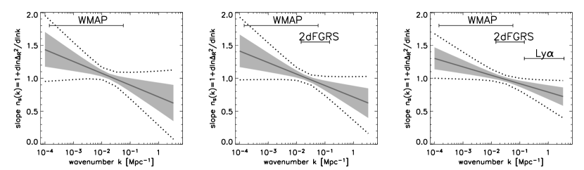
Figure 2: This figure shows $n_{s}$ as a function of $k$ for the WMAP (left), WMAPext+2dFGRS (middle) and WMAPext+2dFGRS$+$Lyman $\alpha$ (right) data sets. The mean (solid line) and the 68% (shaded area) and 95% (dashed lines) intervals are shown. The scales probed by WMAP, 2dFGRS and Lyman $\alpha\$ are indicated on the figure.

Figure 2 shows our constraint on $n_{s}$ as a function of $k$ for the WMAP, WMAPext+ 2dFGRS and WMAPext+ 2dFGRS + Lyman $\alpha$ data sets. At each wavenumber $k$, we use equation (8) to convert $n_{s}(k_{0}=0.002~{}{\rm Mpc}^{-1})$ to $n_{s}(k)$ at each wavenumber. Then, we evaluate the mean (solid line), 68% interval (shaded area), and 95% interval (dashed lines) from the MCMCs. This shows a hint that the spectral index is running from blue ($n_{s}>1$) on large scales to red ($n_{s}<1$) on small scales. In our MCMCs, for the WMAP data set alone, 91% of models explored by the chain have a scalar spectral index running from blue at $k=0.0007\ \mathrm{Mpc^{-1}}$ ($l\sim 10$) to red at $k=2\ \mathrm{Mpc^{-1}}$. For the WMAPext+2dFGRS data set, 95% of models go from a blue index at large scales to a red index at small scales, and when Lyman $\alpha$ forest data is added, the fraction running from blue to red becomes 96%.

One-loop correction and renormalization usually predict running mass and/or running coupling constant, giving some $dn_{s}/d\ln k$. Detection of it implies interesting quantum phenomena during inflation (see Lyth & Riotto (1999) for a review). For the running of the scalar spectral index (equation 22),

$$\frac{dn_{s}}{d\ln k}=-2\xi_{\scriptscriptstyle V}-\frac{2}{3}\left[(n_{s}-1)^{2}-4\eta_{\scriptscriptstyle V}^{2}\right].$$ (24)

Since the data requires $n_{s}\sim 1$ (see Table 1), $(n_{s}-1)^{2}\lesssim 0.01$. It is especially small when $n_{s}-1\simeq 2\eta_{\scriptscriptstyle V}$, (see Case A and Case D in § 3.4.2). Therefore, if $dn_{s}/d\ln k$ is large enough to detect, $dn_{s}/d\ln k>10^{-2}$, then $dn_{s}/d\ln k$ must be dominated by $2\xi_{\scriptscriptstyle V}$, a product of the first and the third derivatives of the potential (equation (17)). The hint of $dn_{s}/d\ln k$ in our data can be interpreted as $\xi_{\scriptscriptstyle V}\simeq-\frac{1}{2}dn_{s}/d\ln k=0.028\pm 0.015$. However, obtaining the running from blue to red, which is suggested by the data, may require fine-tuned properties in the shape of the potential. More data are required to determine whether the hints of a running index are real.

3.4 Single field models confront the data

3.4.1 Testing a specific inflation model: $\lambda\phi^{4}$

As a prelude to showing constraints on broad classes of inflationary models, we first illustrate the power of the data using the example of the minimally-coupled $V=\lambda\phi^{4}/4$ model, which is often used as an introduction to inflationary models (Linde, 1990). We show that this textbook example is unlikely.

The Friedmann and continuity equations for a homogeneous scalar field lead to the slow-roll parameters, which one can use in conjunction with the equations of § 3.2.2 in order to obtain predictions for the observables. For the potential $V(\phi)=\lambda\phi^{4}/4$, one obtains the potential slow roll parameters as:

$$\epsilon_{\scriptscriptstyle V}=8\frac{M_{\rm pl}^{2}}{\phi^{2}},\qquad\eta_{\scriptscriptstyle V}={1}{2}\frac{M_{\rm pl}^{2}}{\phi^{2}},\qquad\xi_{\scriptscriptstyle V}=96\frac{M_{\rm pl}^{4}}{\phi^{4}}.$$ (25)

The number of $e$-foldings remaining till the end of inflation is defined by

$$N=\int_{t}^{t_{end}}Hdt\simeq\frac{1}{M_{\rm pl}^{2}}\int_{\phi_{end}}^{\phi}\frac{V}{V^{\prime}}\ d\phi=\frac{1}{8}\left(\frac{\phi^{2}-\phi_{end}^{2}}{M_{\rm pl}^{2}}\right),$$ (26)

where $\epsilon_{\scriptscriptstyle V}(\phi_{end})=1$ defines the end of inflation. Assuming $\phi_{end}\ll\phi$, taking the horizon exit scale as $\phi\simeq\sqrt{8N}M_{\rm pl}$ and $N=50$, one obtains $n_{s}=0.94$ and $r=0.32$ using equations (19) and (20). As $dn_{s}/d\ln k$ is negligible for this model, we use $dn_{s}/d\ln k=0$.

We maximize the likelihood for this model by running a simulated annealing code. We fit to WMAPext+2dFGRS data, varying the following parameters: $\Omega_{b}h^{2}$, $\Omega_{m}h^{2}$, $h$, $\tau$, $A$, $\beta$, and $\sigma_{p}$, while keeping $n_{s}$, $dn_{s}/d\ln k$, and $r$ fixed at the $\lambda\phi^{4}$ values. The maximum likelihood model obtained has [$\Omega_{b}h^{2}=0.022$, $\Omega_{m}h^{2}=0.135$, $\tau=0.07$, $A=0.67$, $h=0.69$, $\sigma_{8}=0.76$]. This best-fit model is compared in Table 2 to the corresponding model with the full set of single field inflationary parameters. The $\lambda\phi^{4}$ model is displaced from the maximum likelihood generic single field model by $\Delta{\chi^{2}_{eff}}=16$ [$\Delta{\chi^{2}_{eff}}$(WMAP) $=14$, $\Delta{\chi^{2}_{eff}}$(CBI+ACBAR+2dFGRS) $=2$], where ${\chi^{2}_{eff}}=-2\ln{\cal L}$ and ${\cal L}$ is the likelihood (see Verde et al. (2003)). Since the relative likelihood between the models is $\exp(-8)$, and the number of degrees of freedom is approximately three, $\lambda\phi^{4}$ is disfavored at more than $3\sigma$. The table shows that adding external data sets does not make a significant difference to the $\Delta{\chi^{2}_{eff}}$ between the models, and the constraint is primarily coming from WMAP data.

This result holds only for Einstein gravity. When a non-minimal coupling of the form $\xi\phi^{2}R$ ($\xi=1/6$ is the conformal coupling) is added to the Lagrangian, the coupling changes the dynamics of $\phi$. This model predicts only a tiny amount of tensor modes (Komatsu & Futamase, 1999; Hwang & Noh, 1998) in agreement with the data.

Table 2: Goodness-of-fit Comparison for $\lambda\phi^{4}$ Model

Model	${\chi^{2}_{eff}}$ (WMAP)	${\chi^{2}_{eff}}$ (ext+2dFGRS)	Total ${\chi^{2}_{eff}}/\nu$ (WMAPext+2dFGRS)
Best-fit inflation	1428	36	1464/1379
$\lambda\phi^{4}$ model	1442	38	1480/1382

One can perform a similar analysis on any given inflationary model to see what constraints the data put on it. Rather than attempt this Herculean task, in the following section we simply use our constraints on $n_{s}$, $dn_{s}/d\ln k$, and $r$ and the predictions of various classes of single field inflationary models for these parameters in order to put broad constraints on them.

3.4.2 Testing a broad class of inflation models

Naively, the parameter space in observables spanned by the slow roll parameters appears to be large. We shall show below that “viable” slow roll inflation models (i.e. those that can sustain inflation for a sufficient number of $e$-folds to solve cosmological problems) actually occupy significantly smaller regions in the parameter space.

Hoffman & Turner (2001); Kinney (2002a); Easther & Kinney (2002); Hansen & Kunz (2002); Caprini et al. (2003) have investigated generic predictions of slow roll inflation models by using a set of inflationary flow equations (see Appendix A for a detailed description and definition of conventions). In particular Kinney (2002a) and Easther & Kinney (2002) use Monte Carlo simulations to extend the slow roll approximations to fifth order. These authors find “attractors” corresponding to fixed points (where all derivatives of the flow parameters vanish); models cluster strongly near the power-law inflation predictions, $r=8(1-n_{s})$ (see § 3.4.4), and on the zero tensor modes, $r=0$.

Following the method of Kinney (2002a) and Easther & Kinney (2002), we compute a million realizations of the inflationary flow equations numerically, truncating the flow equation hierarchy at eighth order and evaluating the observables to second order in slow roll using equations (A16)–(A18). We marginalize over the ambiguity of converting between $\phi$ and $k$, introduced by the details of reheating and the energy density during inflation by adopting the Monte Carlo approach of the above authors. The observable quantities of a given realization of the flow equations are evaluated at a specific value of $e$-folding, $N$. However, observable quantities are measured at a specific value of $k$. Therefore, we need to relate $N$ to $k$. This requires detailed modeling of reheating, which carries an inherent uncertainty. We attempt to marginalize over this by randomly drawing $N$ values from a uniform distribution $N=[40,70]$.

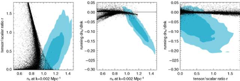
Figure 3: This set of figures shows part of the parameter space spanned by viable slow roll inflation models, with the WMAP 68% confidence region shown in dark blue and the 95% confidence region shown in light blue.

Figure 3 shows part of the parameter space of viable slow roll inflation models, with the WMAP 95% confidence region shown in blue. Each point on these panels is a different Monte Carlo realization of the flow equations, and corresponds to a viable slow roll model. Not all points that are viable slow roll models correspond to specific physical models constructed in the literature. Most of the models cluster near the attractors, sparsely populating the rest of the large parameter space allowed by the slow roll classification. It must be emphasized that these scatter plots should not be interpreted in a statistical sense since we do not know how the initial conditions for the universe are selected. Even if a given realization of the flow equations does not sit on the attractor, this does not mean that it is not favored. Each point on this plot carries equal weight, and each is a viable model of inflation. Notice that the WMAP data do not lie particularly close to the $r=8(1-n_{s})$ “attractor” solution, at the 2-$\sigma$ level, but is quite consistent with the $r=0$ attractor.

One may categorize slow roll models into several classes depending upon where the predictions lie on the parameter space spanned by $n_{s}$, $dn_{s}/d\ln k$, and $r$ (Dodelson et al., 1997; Kinney, 1998; Hannestad et al., 2001). Each class should correspond to specific physical models of inflation. Hereafter, we drop the subscript $V$ unless there is an ambiguity — it should otherwise be implicitly assumed that we are referring to the standard slow roll parameters. We categorize the models on the basis of the curvature of the potential $\eta$, as it is the only parameter that enters into the relation between $n_{s}$ and $r$ (equation (20)), and between $n_{s}$ and $dn_{s}/d\ln k+2\xi$ (equation (22)). Thus, $\eta$ is the most important parameter for classifying the observational predictions of the slow roll models. The classes are defined by

• negative curvature models, $\eta<0$,

• small positive (or zero) curvature models, $0\leq\eta\leq 2\epsilon$,

• intermediate positive curvature models, $2\epsilon<\eta\leq 3\epsilon$, and

• large positive curvature models, $\eta>3\epsilon$.

Each class occupies a certain region in the parameter space. Using $\eta=(n_{s}-1)\alpha/[2(\alpha-3)]$, where $\eta=\alpha\epsilon$, one finds

• $n_{s}<1$, $0\leq r<\frac{8}{3}(1-n_{s})$, $-\frac{2}{3}(1-n_{s})^{2}<dn_{s}/d\ln k+2\xi<0$,

• $n_{s}<1$, $\frac{8}{3}(1-n_{s})\leq r\leq 8(1-n_{s})$, $-\frac{2}{3}(1-n_{s})^{2}\leq dn_{s}/d\ln k+2\xi\leq 2(1-n_{s})^{2}$,

• $n_{s}<1$, $r>8(1-n_{s})$, $dn_{s}/d\ln k+2\xi>2(1-n_{s})^{2}$, and

• $n_{s}\geq 1$, $r\geq 0$, $dn_{s}/d\ln k+2\xi>0$.

To first order in slow roll, the subspace ($n_{s}$, $r$) is uniquely divided into the four classes, and the whole space spanned by these parameters is defined by this classification. The division of the other subspace ($n_{s}$, $dn_{s}/\ln k$) is less unique, and $dn_{s}/d\ln k<-2\xi-\frac{2}{3}(1-n_{s})^{2}$ is not covered by this classification. To higher order in slow roll, these boundaries only hold approximately - for instance, Case C can have a slightly blue scalar index, and Case D can have a slightly red one.

We summarize basic predictions of the above model classes to first order in slow roll using the relation between $r$ and $n_{s}$ (equation (20)) rewritten as

$$r=\frac{8}{3}(1-n_{s})+\frac{16}{3}\eta.$$ (27)

This implies:

• negative curvature models predict $\eta<0$ and $1-n_{s}>0$; the second term nearly cancels the first to give $r$ too small to detect,

• small positive curvature models predict $1-n_{s}>0$ and $\eta>0$; a large $r$ is produced,

• intermediate positive curvature models predict $1-n_{s}>0$ and $\eta>0$; a large $r$ is produced, and

• large positive curvature models predict $1-n_{s}<0$ and $\eta>0$; the first term nearly cancels the second to give $r$ too small to detect.

The cancellation of the terms in Case A and Case D implies $n_{s}-1\simeq 2\eta$: the steepness of the potential in Case A and Case D is insignificant compared to the curvature, $\epsilon\ll\left|\eta\right|$. On the other hand, in Case B and Case C the steepness is larger than or comparable to the curvature, by definition; thus, non-detection of $r$ can exclude many models in Case B and Case C. As we have shown in § 3.4.1, a minimally-coupled $\lambda\phi^{4}$ model, which falls into Case B, is excluded at high significance, largely because of our non-detection of $r$ (see also § 3.4.4).

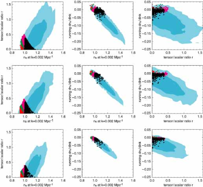
Figure 4: This set of figures compares the fits from the WMAP (top row), WMAPext+2dFGRS (middle row) and WMAPext+2dFGRS+Ly$\alpha$ data (bottom row) to the predictions of specific classes of physically motivated inflation models. The color coding shows model classes referred to in the text: (A) red, (B) green, (C) magenta, (D) black. The dark and light blue regions are the joint 1–$\sigma$ and 2–$\sigma$ regions for the specified data sets (contrast this with the 1-d marginalized 1–$\sigma$ errors given in Table 1). We show only Monte Carlo models that are consistent with all three 2–$\sigma$ regions in each data set. This figure does not imply that the models not plotted are ruled out.

For an overview, Figure 4 shows the Monte Carlo flow equation realizations corresponding to the model classes A–D above on the ($n_{s}$, $r$), ($n_{s}$, $dn_{s}/d\ln k$), and ($r$, $dn_{s}/d\ln k$) planes, for the WMAP, WMAPext+2dFGRS and WMAPext+2dFGRS+Lyman $\alpha$ data sets.

In Table 3, we show the ranges taken by the observables $n_{s}$, $r$ and $dn_{s}/d\ln k$ in the Monte Carlo realizations that remain after throwing out all the points which are outside at least one of the joint-95% confidence levels. These points have been separated into the model classes A–D via their $\eta_{\scriptscriptstyle V}$. These constraints were calculated as follows. First, we find the Monte Carlo realizations of the flow equations from each model class that fall inside all the joint-95% confidence levels for a given data set, separately for the WMAP, WMAPext+2dFGRS and WMAPext+2dFGRS+Lyman $\alpha$ data sets (i.e. the models shown on Figure 4). Then we find for each model class the maximum and minimum values predicted for each of the observables within these subsets. These constraints mean that only those models (within each class) predicting values for the observables that lie outside these limits are excluded by these data sets at 95% CL. Note that the best-fit model within this parameter space has a ${\chi^{2}_{eff}}/\nu=1464/1379$. Here, recall again that the observables were evaluated to second order in slow roll in these calculations. This is the reason that the Class C range in $n_{s}$ goes slightly blue and the Class D range in $n_{s}$ goes slightly red; the divisions of the $\eta_{\scriptscriptstyle V}$ classification are only exact to first order in slow roll.

In the following subsections we will discuss in more detail the constraints on specific physical models that fall into the classes A–D. For a given class, we will plot only the flow equation realizations falling into that category that are consistent with the 95% confidence regions of all the planes ($n_{s}$, $r$), ($n_{s}$, $dn_{s}/d\ln k$) and ($r$, $dn_{s}/d\ln k$).

Table 3: Properties of Inflationary Models Present Within the Joint-95% Confidence Region

Model	WMAP	WMAPext+2dFGRS	WMAPext+2dFGRS$+$Lyman $\alpha$
A	$(4\times 10^{-6})\tablenotemark{b}\leq r\leq 0.14$	$(2\times 10^{-6})\tablenotemark{b}\leq r\leq 0.19$	$(4\times 10^{-6})\tablenotemark{b}\leq r\leq 0.16$
	$0.94\leq n_{s}\leq 1.00$	$0.93\leq n_{s}\leq 1.00$	$0.94\leq n_{s}\leq 1.00$
	$-0.02\leq\$$dn_{s}/d\ln k$$\ \leq 0.02$	$-0.04\leq\$$dn_{s}/d\ln k$$\ \leq 0.02$	$-0.02\leq\$$dn_{s}/d\ln k$$\ \leq 0.004$
B	$(7\times 10^{-3})\tablenotemark{b}\leq r\leq 0.35$	$(7\times 10^{-3})\tablenotemark{b}\leq r\leq 0.32$	$(7\times 10^{-3})\tablenotemark{b}\leq r\leq 0.26$
	$0.94\leq n_{s}\leq 1.01$	$0.93\leq n_{s}\leq 1.01$	$0.94\leq n_{s}\leq 1.01$
	$-0.02\leq\$$dn_{s}/d\ln k$$\ \leq 0.02$	$-0.04\leq\$$dn_{s}/d\ln k$$\ \leq 0.02$	$-0.02\leq\$$dn_{s}/d\ln k$$\ \leq 0.01$
C	$(0.003)\tablenotemark{b}\leq r\leq 0.59$	$(0.003)\tablenotemark{b}\leq r\leq 0.52$	$(0.03)\tablenotemark{b}\leq r\leq 0.46$
	$0.95\leq n_{s}\leq 1.02$	$0.96\leq n_{s}\leq 1.02$	$0.97\leq n_{s}\leq 1.02$
	$-0.04\leq\$$dn_{s}/d\ln k$$\ \leq 0.01$	$-0.04\leq\$$dn_{s}/d\ln k$$\ \leq 0.01$	$-0.04\leq\$$dn_{s}/d\ln k$$\ \leq 0.001$
D	$0.0\leq r\leq 1.10$	$0.0\leq r\leq 0.89$	$(8\times 10^{-5})\tablenotemark{b}\leq r\leq 0.89$
	$0.99\leq n_{s}\leq 1.28$	$1.00\leq n_{s}\leq 1.28$	$1.00\leq n_{s}\leq 1.28$
	$-0.09\leq\$$dn_{s}/d\ln k$$\ \leq 0.03$	$-0.09\leq\$$dn_{s}/d\ln k$$\ \leq 0.01$	$-0.09\leq\$$dn_{s}/d\ln k$$\ \leq-0.001$

Note that very few models predict a “bad power law”, or $|$$dn_{s}/d\ln k$$|>0.05$.

3.4.3 Case A: negative curvature models $\eta<0$

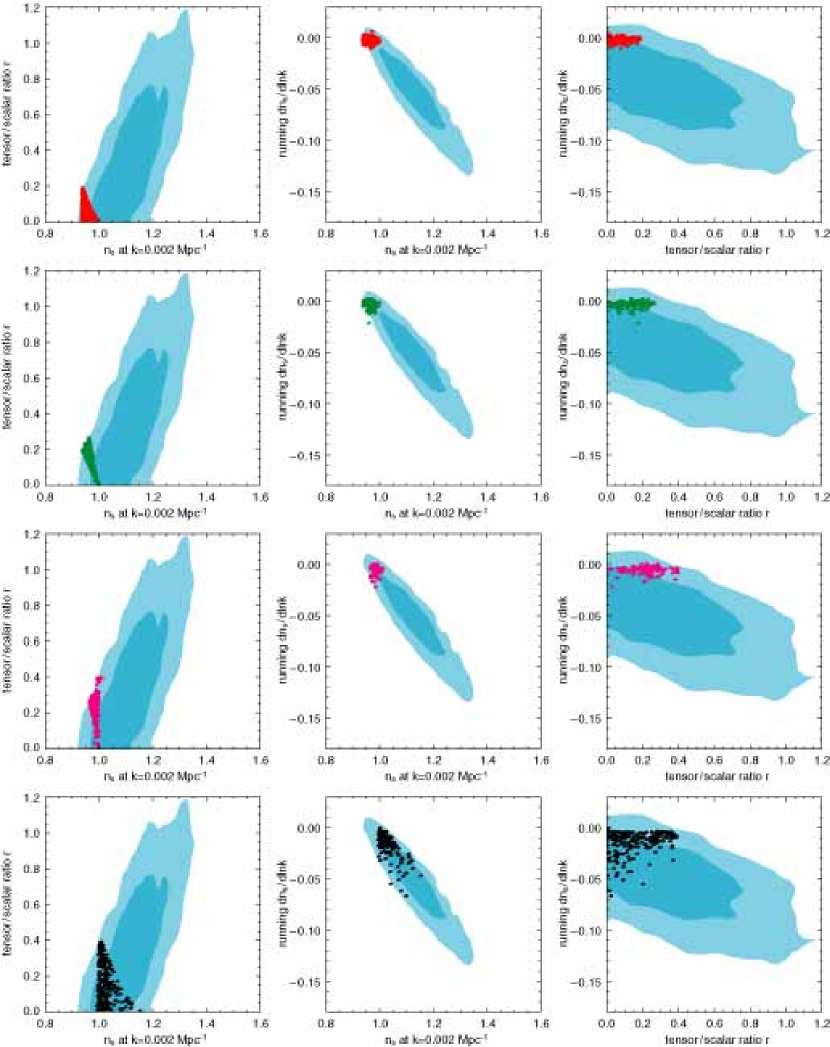
Figure 5: This set of figures compares the fits from the WMAPext+2dFGRS+Ly$\alpha$ data to the predictions of all four classes of inflation models. The top row is Class A [red dots]. The second row is Class B [green dots]. The third row is Class C [magenta dots]. The bottom row is Class D [black dots]. The dark and light blue regions are the joint 1–$\sigma$ and 2–$\sigma$ regions for the WMAPext+2dFGRS+Ly$\alpha$ data. We show only Monte Carlo models that are consistent with 2–$\sigma$ regions in all panels. This figure does not imply that the models not plotted are ruled out.

The top row of Figure 5 shows the Monte Carlo points belonging to Case A which are consistent with all the joint-95% confidence regions of the observables shown in the figure, for the WMAPext+2dFGRS+Lyman $\alpha$ data set.

The negative $\eta$ models often arise from a potential of spontaneous symmetry breaking (e.g., new inflation - Albrecht & Steinhardt (1982); Linde (1982)).

We consider negative-curvature potentials in the form of $V=\Lambda^{4}[1-(\phi/\mu)^{p}]$ where $p\geq 2$. We require $\phi<\mu$ for the form of the potential to be valid, and $\Lambda$ determines the energy scale of inflation, or the energy stored in a false vacuum. One finds that this model always gives a red tilt $n_{s}<1$ to first order in slow roll, as $n_{s}-1=-6\epsilon-2\left|\eta\right|<0$.

For $p=2$, the number of $e$-folds at $\phi$ before the end of inflation is given by $N\simeq(\mu^{2}/2M_{\rm pl}^{2})\ln(\mu/\phi)$, where we have approximated $\phi_{\rm end}\simeq\mu$. By using the same approximation, one finds $n_{s}-1\simeq-4(M_{\rm pl}/\mu)^{2}$, and $r\simeq 32(\phi^{2}M^{2}_{\rm pl}/\mu^{4})\simeq 8(1-n_{s})e^{-N(1-n_{s})}$. In this class of models, $n_{s}$ cannot be very close to 1 without $\mu$ becoming larger than $m_{\rm pl}$. For example, $n_{s}=0.96$ implies $\mu\simeq 10M_{\rm pl}\simeq 2m_{\rm pl}$. For this class of models, $r$ has a peak value of $r\simeq 0.06$ at $n_{s}=0.98$ (assuming $N=50$). Even this peak value is too small for WMAP to detect. We see from Table 3 that this model is consistent with the current data, but requires $\mu>m_{\rm pl}$ to be valid.

For $p\geq 3$, $n_{s}-1\simeq-(2/N)(p-1)/(p-2)$ or $0.92\leq n_{s}<0.96$ for $N=50$ regardless of a value of $\mu$, and $r\simeq 4p^{2}(M_{\rm pl}/\mu)^{2}(\phi/\mu)^{2(p-1)}$ is negligible as $\phi\ll\mu$. These models lie in the joint 2–$\sigma$ contour.

The negative $\eta$ model also arises from the potential in the form of $V=\Lambda^{4}[1+\alpha\ln(\phi/\mu)]$, a one-loop correction in a spontaneously broken supersymmetric theory (Dvali et al., 1994). Here the coupling constant $\alpha$ should be smaller than of order 1. In this model $\phi$ rolls down towards the origin. One finds $n_{s}-1=-(1+\frac{3}{2}\alpha)/N$ which implies $0.95<n_{s}<0.98$ for $1>\alpha>0$ (this formula is not valid when $\alpha=0$ or $\phi=\mu$). Since $r=8\alpha/N=8\alpha(1+\frac{3}{2}\alpha)^{-1}(1-n_{s})=0.016(\alpha/0.1)$, the tensor mode is too small for WMAP to detect, unless the coupling $\alpha$ takes its maximal value, $\alpha\sim 1$. This type of model is consistent with the data.

3.4.4 Case B: small positive curvature models $0\leq\eta\leq 2\epsilon$

The second row of Figure 5 shows the Monte Carlo points belonging to Case B which are consistent with all the joint-95% confidence regions of the observables shown in the figure.

The “small” positive $\eta$ models correspond to monomial potentials for $0<\eta<2\epsilon$ and exponential potentials for $\eta=2\epsilon$. The monomial potentials take the form of $V=\Lambda^{4}(\phi/\mu)^{p}$ where $p\geq 2$, and the exponential potentials $V=\Lambda^{4}\exp(\phi/\mu)$. The zero $\eta$ model is $V=\Lambda^{4}(\phi/\mu)$. To first order in slow roll, the scalar spectral index is always red, as $n_{s}-1=-6\epsilon+2\eta\leq-4\epsilon<0$. The zero $\eta$ model marks a border between the negative $\eta$ models and the positive $\eta$ models, giving $r=\frac{8}{3}(1-n_{s})$.

The monomial potentials often appear in chaotic inflation models (Linde, 1983), which require that $\phi$ be initially displaced from the origin by a large amount, $\sim m_{\rm pl}$, in order to avoid fine-tuned initial values for $\phi$. The monomial potentials can have a period of inflation at $\phi\gtrsim m_{\rm pl}$, and inflation ends when $\phi$ rolls down to near the origin. For $p=2$, inflation is driven by the mass term, which gives $\phi=2\sqrt{N}M_{\rm pl}$, $n_{s}=1-2/N=0.96$, $r=8/N=4(1-n_{s})=0.16$, and $dn_{s}/d\ln k=-2/N^{2}=-(1-n_{s})^{2}/2=-0.8\times 10^{-3}$. For $p=4$, inflation is driven by the self-coupling, which gives $\phi=2\sqrt{2N}M_{\rm pl}$, $n_{s}=1-3/N=0.94$, $r=16/N=\frac{16}{3}(1-n_{s})=0.32$, and $dn_{s}/d\ln k=-3/N^{2}=-(1-n_{s})^{2}/3=-1.2\times 10^{-3}$. The most striking feature of the small positive $\eta$ models is that the gravitational wave amplitude can be large, $r\geq 0.16$. Our data suggest that, for monomial potentials to lie within the joint 95% contour, $r<0.26$ (Table 3). A $\lambda\phi^{4}$ model is excluded at $\sim 3$–$\sigma$ (§ 3.4.1), and any monomial potentials with $p>4$ are also excluded at high signifcance. Models with $p=2$ (mass term inflation) are consistent with the data.

The exponential potentials appear in the Brans–Dicke theory of gravity (Brans & Dicke, 1961; Dicke, 1962) conformally transformed to the Einstein frame (the extended inflation models) (La & Steinhardt, 1989). One finds $n_{s}=1-(\mu/M_{\rm pl})^{2}$, $r=8(1-n_{s})$, and $dn_{s}/d\ln k=0$. Thus, the exponential potentials predict an exact power-law spectrum and significant gravitational waves for significantly tilted spectra. Since $\mu=NM_{\rm pl}^{2}/(\phi-\phi_{end})$, $n_{s}=1-[NM_{\rm pl}/(\phi-\phi_{end})]^{2}$. The 95% range for $n_{s}$ in Table 3 implies that $\phi-\phi_{end}>4NM_{\rm pl}\simeq 200M_{\rm pl}\simeq 40m_{\rm pl}$.

The exponential potentials mark a border between the small positive $\eta$ models and the positive intermediate $\eta$ models described below.

3.4.5 Case D: large positive curvature models $\eta>3\epsilon$

Before describing Case C, it is useful to describe Case D first. The fourth row of Figure 5 shows the Monte Carlo points belonging to Case D which are consistent with all the joint-95% confidence regions of the observables shown in the figure.

The “large” positive curvature models correspond to hybrid inflation models (Linde, 1994), which have recently attracted much attention as an $R$-invariant supersymmetric theory naturally realizes hybrid inflation (Copeland et al., 1994; Dvali et al., 1994). While it is pointed out that supergravity effects add too large an effective mass to the inflaton field to maintain inflation, the minimal Kähler supergravity does not have such a large mass problem (Copeland et al., 1994; Linde & Riotto, 1997). The distinctive feature of this class of models with $\eta>3\epsilon$ is that the spectrum has a blue tilt, $n_{s}-1=-6\epsilon+2\eta>0$, to first order in slow roll.

A typical potential is a monomial potential plus a constant term, $V=\Lambda^{4}[1+(\phi/\mu)^{p}]$, which enables inflation to occur for a small value of $\phi$, $\phi<m_{\rm pl}$. At first sight, inflation never ends for this potential, as the constant term sustains the exponential expansion forever. Hybrid inflation models postulate a second field $\sigma$ which couples to $\phi$. When $\phi$ rolls slowly on the potential, $\sigma$ stays at the origin and has no effect on the dynamics. For a small value of $\phi$ inflation is dominated by a false vacuum term, $V(\phi,\sigma=0)\simeq\Lambda^{4}$. When $\phi$ rolls down to some critical value, $\sigma$ starts moving toward a true vacuum state, $V(\phi,\sigma)=0$, and inflation ends. A numerical calculation (Linde, 1994) suggests that the potential is described by $\phi$ only until $\phi$ reaches a critical value. When $\phi$ reaches the critical value, inflation suddenly ends and $\sigma$ need not be considered. Thus, we include the hybrid models in our discussion of single-field models.

For $p=2$, one finds that $N\simeq\frac{1}{2}(\mu/M_{\rm pl})^{2}\ln(\phi/\phi_{\rm end})\simeq 50$, which, in turn, implies $\mu\sim 10M_{\rm pl}\simeq 2m_{\rm pl}$ for $\ln(\phi/\phi_{\rm end})\sim 1$. The spectral slope is estimated as $n_{s}\simeq 1+4(M_{\rm pl}/\mu)^{2}\sim 1.04$, and the tensor/scalar ratio, $r\simeq 32(\phi/\mu)^{2}(M_{\rm pl}/\mu)^{2}=8(\phi/\mu)^{2}(n_{s}-1)$, is negligible as inflation occurs at $\phi\ll\mu$. The running is also negligible, as $dn_{s}/d\ln k\simeq 64(\phi/\mu)^{2}(M_{\rm pl}/\mu)^{4}=4(\phi/\mu)^{2}(n_{s}-1)^{2}\ll 10^{-2}$. This type of model lies within the joint 95% contours.

One-loop correction in a softly broken supersymmetric theory induces a logarithmically running mass, $V=\Lambda^{4}\left\{1+(\phi/\mu)^{2}\left[1+\alpha\ln(\phi/Q)\right]\right\}$, where $\alpha$ is a coupling constant and $Q$ is a renormalization point. Since $n_{s}$ is practically determined by $V^{\prime\prime}$, this potential gives rise to a logarithmic running of $n_{s}$ (Lyth & Riotto, 1999). These models would lie in the region occupied by the Monte Carlo points that have a large, negative $dn_{s}/d\ln k$. This type of model is consistent with the data.

3.4.6 Case C: intermediate positive curvature models $2\epsilon<\eta\leq 3\epsilon$

The third row of Figure 5 shows the Monte Carlo points belonging to Case C which are consistent with all the joint-95% confidence regions of the observables shown in the figure.

The “intermediate” positive curvature models are defined, to first order in slow roll, as having a red tilt, $n_{s}-1=-6\epsilon+2\eta<0$, or the exactly scale-invariant spectrum, $n_{s}-1=0$, while not being described by monomial or exponential potentials. These conditions lead to a parameter space where $2\epsilon<\eta\leq 3\epsilon$. Here we discuss only examples of physical models that do not solely live in Case C, but briefly pass through it as they transition from Case D to Case B or Case A.

The transition from Case D to Case B may correspond to a special case of hybrid inflation models described in the previous subsection (Case D), $V=\Lambda^{4}[1+(\phi/\mu)^{p}]$. When $\phi\gg\mu$, the potential becomes Case B potential, $V\rightarrow\Lambda^{4}(\phi/\mu)^{p}$, and the spectrum is red, $n_{s}<1$. When $\phi\ll\mu$, the potential drives hybrid inflation, and the spectrum is blue, $n_{s}>1$. On the other hand, when $\phi\sim\mu$, the potential takes a parameter space somewhere between Case B and Case D, which corresponds to Case C. One may argue that this model requires fine-tuned properties in that we just transition from one regime to the other. However, the Case C regime has an interesting property: the spectral index $n_{s}$ runs from red on large scales to blue on small scales, as $\phi$ undergoes the transition from Case B to Case D. This example has the wrong sign for the running of the index compared to the data at the $\sim 2$-$\sigma$ level.

Linde & Riotto (1997) is one example of a transition from Case D to Case A. They consider a supergravity-motivated hybrid potential with a one-loop correction, which can be approximated during inflation as

$$V\simeq\Lambda^{4}\left[1+\alpha\ln(\phi/Q)+\lambda(\phi/\mu)^{4}\right].$$ (28)

Suppose that the one-loop correction is negligible in some early time, i.e., $\phi\simeq Q$. The spectrum is blue. (The third term is practically unimportant, as inflation is driven by the first term at this stage.) If the loop correction becomes important after several $e$-folds, then $n_{s}$ changes from blue to red, as the loop correction gives a red tilt as we saw in § 3.4.3. This example is consistent with the data. The transition (from Case D to Case A) is possible only when $\alpha$ and $Q$ conspire to balance the first term and the second term right at the scale accessible to our observations.

4 MULTIPLE FIELD INFLATION MODELS

4.1 Framework

In general, a candidate fundamental theory of particle physics such as a supersymmetric theory requires not only one, but many other scalar fields. It is thus naturally expected that during inflation there may exist more than one scalar field that contributes to the dynamics of inflation.

In most single-field inflation models, the fluctuations produced have an almost scale-invariant, Gaussian, purely adiabatic power spectrum whose amplitude is characterized by the comoving curvature perturbation, $\hat{\mathcal{R}}$, which remains constant on superhorizon scales. They also predict tensor perturbations with the consistency condition in equation (21).

With the addition of multiple fields, the space of possible predictions widens considerably. The most distinctive feature is the generation of entropy, or isocurvature, perturbations between one field and the other. The entropy perturbation, $\hat{\mathcal{S}}$, can violate the conservation of $\hat{\mathcal{R}}$ on superhorizon scales, providing a source for the late-time evolution of $\hat{\mathcal{R}}$ which weakens the single field consistency condition into an upper bound on the tensor/scalar ratio (Polarski & Starobinsky, 1995; Sasaki & Stewart, 1996; Garcia-Bellido & Wands, 1996). Limits on the possible level of the entropy perturbation thus discriminate between the multiple field models and the single field models. In this section, we consider the minimal extension to single-field inflation – a model consisting of two minimally-coupled scalar fields.

4.2 Correlated Adiabatic/Isocurvature Fluctuations from Double-Field Inflation

The WMAP data confirm that pure isocurvature fluctuations do not dominate the observed CMB anisotropy. They predict large-scale temperature anisotropies that are too large with respect to the measured density fluctuations, and have the wrong peak/trough positions in the temperature and polarization power spectra (Hu & White, 1996; Page et al., 2003). The WMAP observations limit but do not preclude the possibility of correlated mixtures of isocurvature and adiabatic perturbations, which is a generic prediction of two-field inflation models. Both isocurvature and adiabatic perturbations receive significant contributions from at least one of the scalar fields to produce the correlation (Langlois, 1999; Pierpaoli et al., 1999; Langlois & Riazuelo, 2000; Gordon et al., 2001; Bartolo et al., 2001, 2002; Amendola et al., 2002; Wands et al., 2002). We focus on these mixed models in this section.

Let $\hat{\mathcal{R}}_{rad}$ and $\hat{\mathcal{S}}_{rad}$ be the curvature and entropy perturbations deep in the radiation era, respectively. At large scales, the temperature anisotropy is given by (Langlois, 1999):

$$\frac{\Delta T}{T}=\frac{1}{5}\left(\hat{\mathcal{R}}_{rad}-2\hat{\mathcal{S}}_{rad}\right),$$ (29)

in addition to the integrated Sachs–Wolfe effect. The entropy perturbation, $\hat{\mathcal{S}}_{rad}\equiv\delta\rho_{cdm}/\rho_{cdm}-(3/4)\delta\rho_{\gamma}/\rho_{\gamma}$, remains constant on large scales until re-entry into the horizon. If $\hat{\mathcal{R}}_{rad}$ and $\hat{\mathcal{S}}_{rad}$ have the same sign (correlated), then the large scale temperature anisotropy is reduced. If they have opposite signs (anti-correlated), then the temperature anisotropy is increased. Spergel et al. (2003) find that there is an apparent lack of power at the very largest scales in the WMAP data; thus, one of the motivations of this study is to see whether a correlated $\hat{\mathcal{S}}_{rad}$ can provide a better fit to the WMAP low-$l$ data than a purely adiabatic model.

The evolution of the curvature/entropy perturbations from horizon-crossing to the radiation-dominated era can be parameterized by a transfer matrix (Amendola et al., 2002),

$$\left(\begin{array}[]{c}\hat{\mathcal{R}}_{rad}\\ \hat{\mathcal{S}}_{rad}\end{array}\right)=\left(\begin{array}[]{cc}1&T_{RS}\\ 0&T_{SS}\end{array}\right)\left(\begin{array}[]{c}\hat{\mathcal{R}}_{\star}\\ \hat{\mathcal{S}}_{\star}\end{array}\right)_{k=aH}.$$ (30)

Here, $T_{RR}=1$ and $T_{SR}=0$ because of the physical requirement that $\hat{\mathcal{R}}$ is conserved for purely adiabatic perturbations, and that $\hat{\mathcal{R}}$ cannot source $\hat{\mathcal{S}}$. All the quantities in equation (30) are weakly scale-dependent, and may be parameterized by power-laws. Hence, we write this equation as

$$\hat{\mathcal{R}}_{rad} = A_{r}k^{n_{1}}\hat{a_{r}}+A_{s}k^{n_{3}}\hat{a_{s}},$$ (31)

$$\hat{\mathcal{S}}_{rad} = Bk^{n_{2}}\hat{a_{s}},$$ (32)

where $\hat{a_{r}}$ and $\hat{a_{s}}$ are independent Gaussian random variables with unit variance, $\langle\hat{a_{r}}\hat{a_{s}}\rangle=\delta_{rs}$. The cross-correlation spectrum is given by $\Delta^{2}_{RS}(k)\equiv(k^{3}/2\pi^{2})\langle\hat{\mathcal{R}}_{rad}\hat{\mathcal{S}}_{rad}\rangle=A_{s}Bk^{n_{2}+n_{3}}$. One may define the correlation coefficient using an angle $\Delta$ as

$$\cos\Delta\equiv\frac{\langle\hat{\mathcal{R}}_{rad}\hat{\mathcal{S}}_{rad}\rangle}{\langle\hat{\mathcal{R}}^{2}_{rad}\rangle^{1/2}\langle\hat{\mathcal{S}}^{2}_{rad}\rangle^{1/2}}=\frac{\mathrm{sign}(B)A_{s}k^{n_{3}}}{\sqrt{A^{2}_{r}k^{2n_{1}}+A^{2}_{s}k^{2n_{3}}}},$$ (33)

where $-1\leq\cos\Delta\leq 1$. Thus, in general, six parameters ($A_{r}$, $A_{s}$, $\cos\Delta$, $n_{1}$, $n_{2}$, $n_{3}$) are needed to characterize the double-inflation model with correlated adiabatic/isocurvature perturbations, while $\cos\Delta$ is scale-dependent. In order to simplify our analysis, we neglect the scale-dependence of $\cos\Delta$; thus, $n_{1}=n_{3}\neq n_{2}$ and $\cos\Delta=\mathrm{sign}(B)A_{s}/A$. The power spectra are written as $\Delta^{2}_{\cal R}(k)\equiv(k^{3}/2\pi^{2})\langle\hat{{\cal R}}_{rad}^{2}\rangle=(A_{r}^{2}+A_{s}^{2})k^{2n_{1}}\equiv A^{2}k^{n_{ad}-1}$, and $\Delta^{2}_{\cal S}(k)\equiv(k^{3}/2\pi^{2})\langle\hat{{\cal S}}_{rad}^{2}\rangle=B^{2}k^{2n_{2}}\equiv A^{2}f_{iso}^{2}k^{n_{iso}-1}$. We have defined $n_{ad}-1\equiv 2n_{1}$ and $n_{iso}-1\equiv 2n_{2}$ to coincide with the standard notation for the scalar spectral index. The “isocurvature fraction” defined by $f_{iso}\equiv B/A$ determines the relative amplitude of $\hat{{\cal S}}$ to $\hat{{\cal R}}$. The cross-correlation spectrum is then written as $\Delta^{2}_{RS}(k)=\cos\Delta\sqrt{\Delta^{2}_{\cal R}(k)\Delta^{2}_{\cal S}(k)}=A^{2}f_{iso}\cos\Delta\ k^{(n_{ad}+n_{iso})/2-1}$.

The temperature and polarization anisotropies are given by these power spectra:

$$C_{l}^{ad} \propto A^{2}\int\frac{dk}{k}\left(\frac{k}{k_{0}}\right)^{n_{ad}-1}\left[g_{l}^{ad}(k)\right]^{2},$$ (34)

$$C_{l}^{iso} \propto A^{2}f_{iso}^{2}\int\frac{dk}{k}\left(\frac{k}{k_{0}}\right)^{n_{iso}-1}\left[g_{l}^{iso}(k)\right]^{2},$$ (35)

$$C_{l}^{corr} \propto A^{2}f_{iso}\cos\Delta\int\frac{dk}{k}\left(\frac{k}{k_{0}}\right)^{(n_{ad}+n_{iso})/2-1}\left[g_{l}^{ad}(k)g_{l}^{iso}(k)\right],$$ (36)

and the total anisotropy is $C_{l}^{tot}=C_{l}^{ad}+C_{l}^{iso}+2C_{l}^{corr}$. Here, $g_{l}(k)$ is the radiation transfer function appropriate to adiabatic or isocurvature perturbations of either temperature or polarization anisotropies. Note that the quantities $n_{ad}$, $n_{iso}$, and $f_{iso}$ are defined at a specific wavenumber $k_{0}$, which we take to be $k_{0}=\mathrm{0.05\ Mpc^{-1}}$ in the MCMC. To translate the constraint on $f_{iso}$ to any other wavenumber, one uses

$$f_{iso}(k_{1})=f_{iso}(k_{0})\left(\frac{k_{1}}{k_{0}}\right)^{(n_{iso}-n_{ad})/2}.$$ (37)

We can restrict $f_{iso}\geq 0$ without loss of generality. Since we can remove $A$ by normalizing to the overall amplitude of fluctuations in the WMAP data, we are left with 4 parameters, $n_{ad}$, $n_{iso}$, $f_{iso}$, and $\cos\Delta$. We neglect the contribution of tensor modes, as the addition of tensors goes in the opposite direction in terms of explaining the low amplitude of the low-$l$ TT power spectrum. We also neglect the scale-dependence of $n_{ad}$ and $n_{iso}$, as they are not well constrained by our data sets.

We fit to the WMAPext+2dFGRS and WMAPext+2dFGRS+Lyman $\alpha$ data sets with the 11 parameter model ($\Omega_{b}h^{2}$, $\Omega_{m}h^{2}$, $h$, $\tau$, $n_{ad}$, $n_{iso}$, $f_{iso}$, $\cos\Delta$, $A$, $\beta$, $\sigma_{p}$). The results of the fit for the double inflation model parameters are shown in Table 4. Figure  6 shows the cumulative distribution of $f_{iso}$. The best-fit non-primordial cosmological parameter constraints are very similar to the single field case.

Table 4: Cosmological Parameters: Adiabatic + Isocurvature Model

Parameter	WMAPext+2dFGRS	WMAPext+2dFGRS$+$Lyman $\alpha$
$f_{iso}(k_{0}=0.05~{}{\rm Mpc}^{-1})$	$<0.32$	$<0.33$
$n_{ad}$	$0.97\pm 0.03$	$0.95\pm 0.03$
$n_{iso}$	$1.26_{-0.57}^{+0.51}$	$1.29_{-0.56}^{+0.50}$
$\cos\Delta$	$-0.76_{-0.14}^{+0.18}$	$-0.76_{-0.16}^{+0.18}$
$A(k_{0}=0.05~{}{\rm Mpc}^{-1})$	$0.82\pm 0.10$	$0.78\pm 0.08$
$\Omega_{b}h^{2}$	$0.023\pm 0.001$	$0.023\pm 0.001$
$\Omega_{m}h^{2}$	$0.133\pm 0.007$	$0.131\pm 0.006$
$h$	$0.072\pm 0.04$	$0.072\pm 0.04$
$\tau$	$0.16\pm 0.06$	$0.14\pm 0.06$
$\sigma_{8}$	$0.84\pm 0.06$	$0.81\pm 0.04$

While the fit tries to reduce the large-scale anisotropy with an admixture of correlated isocurvature modes as expected (note that $\cos\Delta<0$ corresponds to $\hat{\mathcal{R}}_{rad}$ and $\hat{\mathcal{S}}_{rad}$ having the same sign, from the definition of initial conditions in the CMBFAST code), this only leads to a small reduction in amplitude at the quadrupole. Table 5 compares the goodness-of-fit for this model along with the maximum likelihood models for the $\Lambda$CDM and single field inflation cases. Because ${\chi^{2}_{eff}}/\nu$ is not improved by the addition of three new parameters and considerable physical complexity, we conclude that the data do not require this model. This implies that the initial conditions are consistent with being fully adiabatic.

Table 5: Goodness-of-Fit Comparison for Adiabatic/Isocurvature Model

Model	${\chi^{2}_{eff}}/\nu$
$\Lambda$CDM	1468/1381
Single field inflation	1464/1379
Adiabatic/Isocurvature	1468/1378

5 SMOOTHNESS OF THE INFLATON POTENTIAL

Spergel et al. (2003) point out that there are several sharp features in the WMAP TT angular power spectrum that contribute to the reduced-${\chi^{2}_{eff}}$ for the best-fit model being $\sim 1.09$. The large ${\chi^{2}_{eff}}$ may result from neglecting 0.5–1% contributions to the WMAP TT power spectrum covariance matrix; for example, gravitational lensing of the CMB, beam asymmetry, and non-Gaussianity in noise maps. When included, these effects will likely improve the reduced-${\chi^{2}_{eff}}$ of the best-fit $\Lambda$CDM model. At the moment we cannot attach any astrophysical reality to these features. Similar features appear in Monte Carlo simulations.

While we do not claim these glitches are cosmologically significant, it is intriguing to consider what they might imply if they turn out to be significant after further scrutiny.

In this section we investigate whether the reduced-${\chi^{2}_{eff}}$ is improved by trying to fit one or more of these “glitches” with a feature in the inflationary potential. Adams et al. (1997) show that a class of models derived from supergravity theories naturally gives rise to inflaton potentials with a large number of sudden downward steps. Each step corresponds to a symmetry-breaking phase transition in a field coupled to the inflaton, since the mass changes suddenly when each transition occurs. If inflation occurred in the manner suggested by these authors, a spectral feature is expected every 10-15 $e$-folds. Therefore, one of these features may be visible in the CMB or large-scale structure spectra.

We use the formalism adopted by Adams et al. (2001), and model the step by the potential

$$V_{step}(\phi)=\frac{1}{2}m^{2}\phi^{2}\left[1+c\tanh\left(\frac{\phi-\phi_{s}}{d}\right)\right],$$ (38)

where $\phi$ is the inflaton field, and the potential has a step starting at $\phi_{s}$ with amplitude and gradient determined by $c$ and $d$ respectively. In physically realistic models, the presence of the step does not interrupt inflation, but affects density perturbations by introducing scale-dependent oscillations. Adams et al. (2001) describe the phenomenology of these models: the sharper the step, the larger the amplitude and longevity of the “ringing.” For our calculations of the power spectrum in these models, we numerically integrate the Klein–Gordon equation using the prescription of Adams et al. (2001).

We also phenomenologically model a dip in the inflaton potential using a toy model of a Gaussian dip centered at $\phi_{s}$ with height $c$ and width $d$:

$$V_{dip}(\phi)=\frac{1}{2}m^{2}\phi^{2}\left(1-c\ \exp\left[\frac{(\phi-\phi_{s})^{2}}{2d^{2}}\right]\right).$$ (39)

We fix the non-primordial cosmological parameters at the maximum likelihood values for the $\Lambda$CDM model fitted to the WMAPext data, [$\Omega_{b}h^{2}=0.022$, $\Omega_{m}h^{2}=0.13$, $\tau=0.11$, $A=0.74$, $h=0.72$]. We then run simulated annealing codes for only the three parameters: $\phi_{s}$, $c$, and $d$, for each potential, fitting to the WMAP TT and TE data only. For this section, since this model predicts sharp features in the angular power spectrum, we had to modify the standard CMBFAST splining resolution, splining at $\Delta l=1$ for $2\leq l<50$ and $\Delta l=5$ for $l\geq 50$.

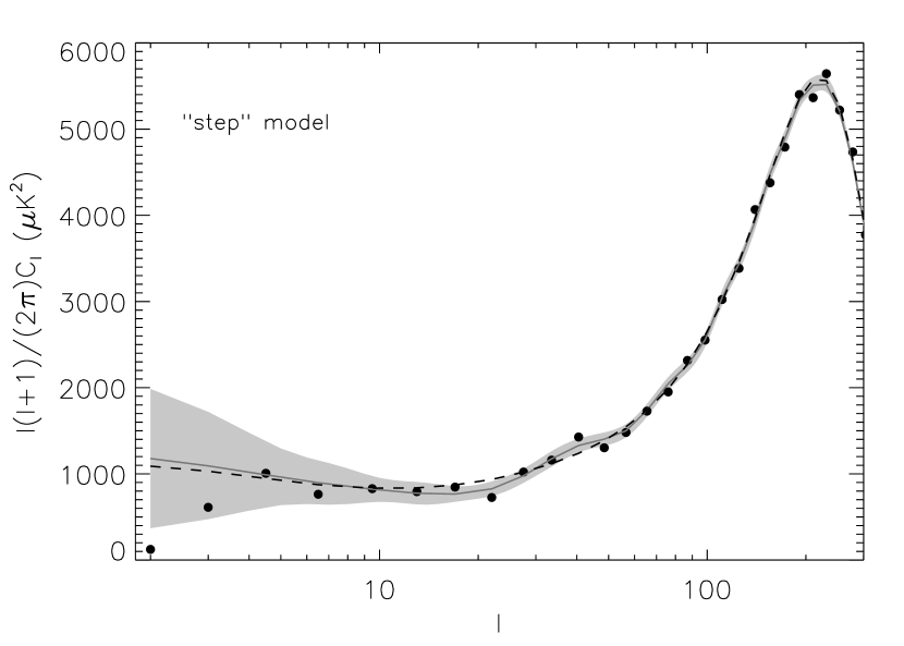
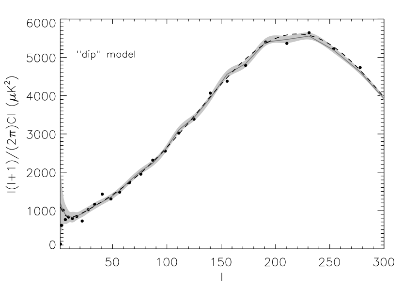
Figure 7: Best-fit models (solid) with a step (left) and a dip (right) in the inflaton potential, with the WMAP TT data. The best-fit $\Lambda$CDM model to WMAPext data is shown (dotted) for comparison.

The best-fit parameters found for each potential are given in Table 6, along with the ${\chi^{2}_{eff}}$ for the WMAP TT and TE data. Figure 7 shows these models plotted along with the WMAP TT data. The best-fit models predict features in the TE spectrum at specific multipoles, which are well below detection, given the current uncertainties. The step model differs from the $\Lambda$CDM model by $\Delta{\chi^{2}_{eff}}=10$, the dip model by $\Delta{\chi^{2}_{eff}}=6$. We are not claiming that these are the best possible models in this parameter space, only that these are the best-fit models found in 8 simulated annealing runs. Note that the models with features were not allowed the freedom to improve the fit by adjusting the cosmological parameters.

Table 6: Best-Fit Models with Potential Features

Model	$\phi_{s}$ ($M_{\rm pl}$)	$c$	$d$ ($M_{\rm pl}$)	WMAP ${\chi^{2}_{eff}}/\nu$
Step	15.5379	0.00091	0.01418	1422/1339
Dip	15.51757	0.00041	0.00847	1426/1339
$\Lambda$CDM	N/A	N/A	N/A	1432/1342

A very small fractional change in the inflaton potential amplitude, $c\sim 0.1$%, is sufficient to cause sharp features in the angular power spectrum. Models with much larger $c$ would have dramatic effects that are not seen in the WMAP angular power spectrum.

These models also predict sharp features in the large-scale structure power spectrum. Figure 8 shows the matter power spectra for the best-fit step/dip models. Forthcoming large-scale structure surveys may look for the presence of such features, and test the viability of these models.

6 CONCLUSIONS

WMAP has made six key observations that are of importance in constraining inflationary models.

• The universe is consistent with being flat (Spergel et al., 2003).

• The primordial fluctuations are described by random Gaussian fields (Komatsu et al., 2003).

• We have shown that the WMAP detection of an anti-correlation between CMB temperature and polarization fluctuations at $\theta>2^{\circ}$ is a distinctive signature of adiabatic fluctuations on superhorizon scales at the epoch of decoupling. This detection agrees with a fundamental prediction of the inflationary paradigm.

• In combination with complementary CMB data (the CBI and the ACBAR data), the 2dFGRS large-scale structure data, and Lyman $\alpha$ forest data, WMAP data constrain the primordial scalar and tensor power spectra predicted by single-field inflationary models. For the scalar modes, the mean and the 68% error level of the 1–d marginalized likelihood for the power spectrum slope and the running of the spectral index are, respectively, $n_{s}(k_{0}=0.002~{}{\rm Mpc}^{-1})=1.13\pm 0.08$ and $dn_{s}/d\ln{k}=-0.055^{+0.028}_{-0.029}$. This value is in agreement with $dn_{s}/d\ln{k}=-0.031^{+0.016}_{-0.018}$ of Spergel et al. (2003), which was obtained for a $\Lambda$CDM model with no tensors and a running spectral index. The data suggest at the 2-$\sigma$ level, but do not require that, the scalar spectral index runs from $n_{s}>1$ on large scales to $n_{s}<1$ on small scales. If true, the third derivative of the inflaton potential would be important in describing its dynamics.

• The WMAPext+2dFGRS constraints on $n_{s}$, $dn_{s}/d\ln k$, and $r$ put limits on single-field inflationary models that give rise to a large tensor contribution and a red ($n_{s}<1$) tilt. A minimally-coupled $\lambda\phi^{4}$ model lies more than 3-$\sigma$ away from the maximum likelihood point. The contribution to the $\Delta\chi^{2}$ between the two points from WMAP  alone is 14.

• We test two-field inflationary models with an admixture of adiabatic and CDM isocurvature components. The data do not justify adding the additional parameters needed for this model, and the initial conditions are consistent with being purely adiabatic.

WMAP both confirms the basic tenets of the inflationary paradigm and begins to quantitatively test inflationary models. However, we cannot yet distinguish between broad classes of inflationary theories which have different physical motivations. In order to go beyond model building and learn something about the physics of the early universe, it is important to be able to make such distinctions at high significance. To accomplish this, one requirement is a better measurement of the fluctuations at high $l$, and a better measurement of $\tau$, in order to break the degeneracy between $n_{s}$ and $\tau$.

We note that an exact scale-invariant spectrum ($n_{s}=1$ and $dn_{s}/d\ln k=0$) is not yet excluded at more than 2$\sigma$ level. Excluding this point would have profound implications in support of inflation, as physical single field inflationary models predict non-zero deviation from exact scale-invariance.

We conclude by showing the tensor temperature and polarization power spectra for the maximum likelihood single-field inflation model for the WMAPext+2dFGRS+Lyman $\alpha$ data set, which has tensor/scalar ratio $r=0.42$ (Figure 9). The detection and measurement of the gravity-wave power spectrum would provide the next important key test of inflation.

Appendix A INFLATIONARY FLOW EQUATIONS

We begin by describing the hierarchy of inflationary flow equations described by the generalized “Hubble Slow Roll” (HSR) parameters. In the Hamilton-Jacobi formulation of inflationary dynamics, one expresses the Hubble parameter directly as a function of the field $\phi$ rather than a function of time, $H\equiv H(\phi)$, under the assumption that $\phi$ is monotonic in time. Then the equations of motion for the field and background are given by:

$$\dot{\phi} = -2M_{\rm pl}^{2}H^{\prime}(\phi),$$ (A1)

$$\left[H^{\prime}(\phi)\right]^{2}-\frac{3}{2M_{\rm pl}^{2}}H^{2}(\phi) = -\frac{1}{2M_{\rm pl}^{4}}V(\phi).$$ (A2)

Here, prime denotes derivatives with respect to $\phi$. Equation (A2), referred to as the Hamilton-Jacobi Equation, allows us to consider inflation in terms of $H(\phi)$ rather than $V(\phi)$. The former, being a geometric quantity, describes inflation more naturally. Given $H(\phi)$, equation (A2) immediately gives $V(\phi)$, and one obtains $H(t)$ by using equation (A1) to convert between $H^{\prime}$ and $\dot{H}$. This can then be integrated to give $a(t)$ if desired, since $H(t)\equiv\dot{a}/a$. Rewriting equation (A2) as

$$H^{2}(\phi)\left[1-\frac{1}{3}\epsilon_{\scriptscriptstyle H}\right]=\frac{1}{3M_{\rm pl}^{2}}V(\phi),$$ (A3)

we obtain

$$\left(\frac{\ddot{a}}{a}\right) = \frac{1}{3M_{\rm pl}^{2}}[V(\phi)-\dot{\phi}^{2}]$$

$$= H^{2}(\phi)[1-\epsilon_{\scriptscriptstyle H}(\phi)],$$

so that the condition for inflation $(\ddot{a}/a)>0$ is simply given by $\epsilon_{\scriptscriptstyle H}<1$.

Thus, one can define a set of HSR parameters in analogy to the PSR parameters of § 3.2.2, though there is no assumption of slow-roll implicit in this definition:

$$\epsilon_{\scriptscriptstyle H} \equiv 2M_{\rm pl}^{2}\left(\frac{H^{\prime}(\phi)}{H(\phi)}\right)^{2}$$ (A4)

$$\eta_{\scriptscriptstyle H} \equiv 2M_{\rm pl}^{2}\left(\frac{H^{\prime\prime}(\phi)}{H(\phi)}\right)$$ (A5)

$$\xi_{\scriptscriptstyle H} \equiv 4M_{\rm pl}^{4}\left(\frac{H^{\prime}(\phi)H^{\prime\prime\prime}(\phi)}{H^{2}(\phi)}\right)$$ (A6)

$${}^{\ell}\lambda_{\scriptscriptstyle H} \equiv \left(2M_{\rm pl}\right)^{\ell}\frac{(H^{\prime})^{\ell-1}}{H^{\ell}}\frac{d^{(\ell+1)}H}{d\phi^{(\ell+1)}}.$$ (A7)

We need one more ingredient; the number of $e$-folds before the end of inflation, $N$ is defined by,

$$N\equiv\int_{t}^{t_{e}}H\ dt=\int_{\phi}^{\phi_{e}}\frac{H}{\dot{\phi}}\ d\phi=\frac{1}{\sqrt{2}M_{\rm pl}}\int^{\phi}_{\phi_{e}}\frac{d\phi}{\sqrt{\epsilon_{\scriptscriptstyle H}(\phi)}},$$ (A8)

where $t_{e}$ and $\phi_{e}$ are the time and field value at the end of inflation, and $N$ increases the earlier one goes back in time ($t>0\Rightarrow dN<0$). The derivative with respect to $N$ is therefore,

$$\frac{d}{dN}=\frac{M_{\rm pl}}{2}\sqrt{\epsilon}\frac{d}{d\phi}.$$ (A9)

Then, an infinite hierarchy of inflationary “flow” equations can be defined by differentiating equations (A4)–(A7) with respect to $N$:

$$\frac{d\epsilon_{\scriptscriptstyle H}}{dN} = 2\epsilon_{\scriptscriptstyle H}(\eta_{\scriptscriptstyle H}-\epsilon_{\scriptscriptstyle H})$$ (A10)

$$\frac{d(^{\ell}\lambda_{\scriptscriptstyle H})}{dN} = \begin{array}[]{cr}\left[(\ell-1)\eta_{\scriptscriptstyle H}-\ell\epsilon_{\scriptscriptstyle H}\right](^{\ell}\lambda_{\scriptscriptstyle H})+\ ^{\ell+1}\lambda_{\scriptscriptstyle H}&(\ell>0)\end{array}.$$ (A12)

The definition of the scalar and tensor power spectra are:

$$\Delta^{2}_{\cal R} = \left[\left(\frac{H}{\dot{\phi}}\right)\left(\frac{H}{2\pi}\right)\right]^{2}_{k=aH}$$ (A13)

$$\Delta^{2}_{h} = \frac{8}{M_{\rm pl}^{2}}\left(\frac{H}{2\pi}\right)^{2}_{k=aH}.$$ (A14)

Since derivatives with respect to wavenumber $k$ can be expressed with respect to $N$ as:

$$\frac{d}{dN}=-(1-\epsilon_{\scriptscriptstyle H})\frac{d}{d\ln k},$$ (A15)

the observables are given in terms of the HSR parameters to second order as (Stewart & Lyth, 1993; Liddle et al., 1994),

$$r = 16\epsilon_{\scriptscriptstyle H}\left[1+2C(\epsilon_{\scriptscriptstyle H}-\eta_{\scriptscriptstyle H})\right]$$ (A16)

$$n_{s}-1 = (2\eta_{\scriptscriptstyle H}-4\epsilon_{\scriptscriptstyle H})\left[1-\frac{1}{4}(3-5C)\epsilon_{\scriptscriptstyle H}\right]-(3-5C)\epsilon_{\scriptscriptstyle H}^{2}+\frac{1}{2}(3-C)\xi_{\scriptscriptstyle H}$$ (A17)

$$\frac{dn_{s}}{d\ln k} = -\left(\frac{1}{1-\epsilon_{\scriptscriptstyle H}}\right)\frac{dn_{s}}{dN},$$ (A18)

where $C\equiv 4(\ln 2+\gamma)-5$ and $\gamma\simeq 0.577$ is Euler’s constant. Note that, as pointed out in Kinney (2002b), there is a typographical error in defining $C$ in Liddle et al. (1994) that was inherited by Kinney (2002a). We have used the correct value from Stewart & Lyth (1993).

Finally, the PSR parameters are given in terms of the HSR parameters to first order in slow roll as:

$$\epsilon_{\scriptscriptstyle H} = \epsilon_{\scriptscriptstyle V}$$ (A19)

$$\eta_{\scriptscriptstyle H} = \eta_{\scriptscriptstyle V}-\epsilon_{\scriptscriptstyle V}$$ (A20)

$$\xi_{\scriptscriptstyle H} = \xi_{\scriptscriptstyle V}-3\epsilon_{\scriptscriptstyle V}\eta_{\scriptscriptstyle V}+3\epsilon_{\scriptscriptstyle V}^{2}.$$ (A21)

Figure 1: Temperature-Polarization angular power spectrum. The large-angle TE power spectrum predicted in primordial adiabatic models (solid), primordial isocurvature models (dashed), and in causal scaling seed models (dotted). The WMAP TE data (Kogut et al., 2003) is shown for comparison, in bins of $\Delta l=10$.

Figure 6: The cumulative distribution of the isocurvature fraction, $f_{iso}$, for the WMAPext+2dFGRS+Lyman $\alpha$ data set.

Figure 8: The large-scale structure power spectra for the best-fit potential step (left) and dip (right) models.

Figure 9: The tensor power spectrum for the maximum likelihood model from a fit to WMAPext+2dFGRS data sets. The plot shows the TT (solid), EE (dots), BB (short dashes) and the absolute value of TE negative (dots and dashes) and positive (long dashes) tensor spectra.

References

- Adams et al. (2001) Adams, J., Cresswell, B., & Easther, R. 2001, Phys. Rev., D64, 123514
- Adams et al. (1997) Adams, J. A., Ross, G. G., & Sarkar, S. 1997, Phys. Lett., B391, 271
- Albrecht et al. (1996) Albrecht, A., Coulson, D., Ferreira, P., & Magueijo, J. 1996, Phys. Rev. Lett., 76, 1413
- Albrecht & Steinhardt (1982) Albrecht, A. & Steinhardt, P. J. 1982, Phys. Rev. Lett., 48, 1220
- Amendola et al. (2002) Amendola, L., Gordon, C., Wands, D., & Sasaki, M. 2002, Phys. Rev. Lett., 88, 211302
- Bardeen et al. (1983) Bardeen, J. M., Steinhardt, P. J., & Turner, M. S. 1983, Phys. Rev. D, 28, 679
- Bartolo et al. (2001) Bartolo, N., Matarrese, S., & Riotto, A. 2001, Phys. Rev., D64, 123504
- Bartolo et al. (2002) —. 2002, Phys. Rev., D65, 103505
- Birrell & Davies (1982) Birrell, N. D. & Davies, P. C. W. 1982, Quantum fields in curved space (Cambridge University Press)
- Brans & Dicke (1961) Brans, C. & Dicke, R. H. 1961, Physical Review, 124, 925
- Caprini et al. (2003) Caprini, C., Hansen, S. H., & Kunz, M. 2003, MNRAS, 339, 212
- Copeland et al. (1994) Copeland, E. J., Liddle, A. R., Lyth, D. H., Stewart, E. D., & Wands, D. 1994, Phys. Rev., D49, 6410
- Croft et al. (2002) Croft, R. A. C., Weinberg, D. H., Bolte, M., Burles, S., Hernquist, L., Katz, N., Kirkman, D., & Tytler, D. 2002, ApJ, 581, 20
- Dicke (1962) Dicke, R. H. 1962, Physical Review, vol. 125, Issue 6, pp. 2163-2167, 125, 2163
- Dodelson et al. (1997) Dodelson, S., Kinney, W. H., & Kolb, E. W. 1997, Phys. Rev., D56, 3207
- Durrer et al. (2002) Durrer, R., Kunz, M., & Melchiorri, A. 2002, Phys. Rept., 364, 1
- Dvali et al. (1994) Dvali, G. R., Shafi, Q., & Schaefer, R. 1994, Phys. Rev. Lett., 73, 1886
- Easther & Kinney (2002) Easther, R. & Kinney, W. H. 2002, Phys. Rev. D, submitted (astro-ph/0210345)
- Garcia-Bellido & Wands (1996) Garcia-Bellido, J. & Wands, D. 1996, Phys. Rev., D53, 5437
- Gasperini & Veneziano (1993) Gasperini, M. & Veneziano, G. 1993, Astropart. Phys., 1, 317
- Gnedin & Hamilton (2002) Gnedin, N. Y. & Hamilton, A. J. S. 2002, MNRAS, 334, 107
- Gordon et al. (2001) Gordon, C., Wands, D., Bassett, B. A., & Maartens, R. 2001, Phys. Rev., D63, 023506
- Gratton et al. (2003) Gratton, S., Khoury, J., Steinhardt, P., & Turok, N. 2003, preprint (astro-ph/0301395)
- Guth (1981) Guth, A. H. 1981, Phys. Rev. D, 23, 347
- Guth & Pi (1982) Guth, A. H. & Pi, S. Y. 1982, Phys. Rev. Lett., 49, 1110
- Hannestad et al. (2001) Hannestad, S., Hansen, S. H., & Villante, F. L. 2001, Astroparticle Physics, 16, 137
- Hansen & Kunz (2002) Hansen, S. H. & Kunz, M. 2002, MNRAS, 336, 1007
- Hawking (1982) Hawking, S. W. 1982, Phys. Lett., B115, 295
- Hinshaw et al. (2003) Hinshaw, G. F. et al. 2003, ApJ, submitted
- Hoffman & Turner (2001) Hoffman, M. B. & Turner, M. S. 2001, Phys. Rev., D64, 023506
- Hu & Sugiyama (1995) Hu, W. & Sugiyama, N. 1995, ApJ, 444, 489
- Hu & White (1996) Hu, W. & White, M. 1996, ApJ, 471, 30
- Hu & White (1997) —. 1997, Phys. Rev. D, 56, 596
- Hwang & Noh (1998) Hwang, J. & Noh, H. 1998, Physical Review Letters, Volume 81, Issue 24, December 14, 1998, pp.5274-5277, 81, 5274
- Khoury et al. (2002) Khoury, J., Ovrut, B. A., Seiberg, N., Steinhardt, P. J., & Turok, N. 2002, Phys. Rev., D65, 086007
- Khoury et al. (2001) Khoury, J., Ovrut, B. A., Steinhardt, P. J., & Turok, N. 2001, Phys. Rev., D64, 123522
- Kinney (1998) Kinney, W. H. 1998, Phys. Rev., D58, 123506
- Kinney (2002a) —. 2002a, Phys. Rev., D66, 083508
- Kinney (2002b) —. 2002b, preprint (astro-ph/0206032)
- Kogut et al. (2003) Kogut, A. et al. 2003, ApJ, submitted
- Komatsu & Futamase (1999) Komatsu, E. & Futamase, T. 1999, Phys. Rev., D59, 064029
- Komatsu et al. (2003) Komatsu, E. et al. 2003, ApJ, submitted
- Kuo et al. (2002) Kuo, C. L. et al. 2002, ApJ, astro-ph/0212289
- La & Steinhardt (1989) La, D. & Steinhardt, P. J. 1989, Phys. Rev. Lett., 62, 376
- Langlois (1999) Langlois, D. 1999, Phys. Rev., D59, 123512
- Langlois & Riazuelo (2000) Langlois, D. & Riazuelo, A. 2000, Phys. Rev., D62, 043504
- Leach et al. (2002) Leach, S. M., Liddle, A. R., Martin, J., & Schwarz, D. J. 2002, Phys. Rev. D, 66, 23515
- Lewis et al. (2000) Lewis, A., Challinor, A., & Lasenby, A. 2000, ApJ, 538, 473
- Liddle & Lyth (1992) Liddle, A. R. & Lyth, D. H. 1992, Phys. Lett., B291, 391
- Liddle & Lyth (1993) —. 1993, Phys. Rept., 231, 1
- Liddle & Lyth (2000) —. 2000, Cosmological inflation and large-scale structure (Cambridge University Press)
- Liddle et al. (1994) Liddle, A. R., Parsons, P., & Barrow, J. D. 1994, Phys. Rev., D50, 7222
- Linde (1982) Linde, A. D. 1982, Phys. Lett., B108, 389
- Linde (1983) —. 1983, Phys. Lett., B129, 177
- Linde (1990) —. 1990, Particle physics and inflationary cosmology (Chur, Switzerland: Harwood)
- Linde (1994) —. 1994, Phys. Rev., D49, 748
- Linde & Riotto (1997) Linde, A. D. & Riotto, A. 1997, Phys. Rev., D56, 1841
- Lyth & Riotto (1999) Lyth, D. H. & Riotto, A. 1999, Phys. Rept., 314, 1
- Magueijo et al. (1996) Magueijo, J., Albrecht, A., Coulson, D., & Ferreira, P. 1996, Phys. Rev. Lett., 76, 2617
- Mukhanov & Chibisov (1981) Mukhanov, V. F. & Chibisov, G. V. 1981, JETP Letters, 33, 532
- Mukhanov et al. (1992) Mukhanov, V. F., Feldman, H. A., & Brandenberger, R. H. 1992, Phys. Rept., 215, 203
- Mukherjee & Wang (2003a) Mukherjee, P. & Wang, Y. 2003a, 1562, ApJ, submitted (astro-ph/0301562)
- Mukherjee & Wang (2003b) —. 2003b, 1058, ApJ, submitted (astro-ph/0301058)
- Page et al. (2003) Page, L. et al. 2003, ApJ, submitted
- Parker (1969) Parker, L. 1969, Phys. Rev., 183, 1057
- Pearson et al. (2002) Pearson, T. J., et al. 2002, ApJ, submitted (astro-ph/0205388)
- Peebles & Yu (1970) Peebles, P. J. E. & Yu, J. T. 1970, ApJ, 162, 815
- Pen et al. (1994) Pen, U.-L., Spergel, D. N., & Turok, N. 1994, Phys. Rev., D49, 692
- Percival et al. (2001) Percival, W. J., et al. 2001, MNRAS, 327, 1297
- Pierpaoli et al. (1999) Pierpaoli, E., Garcia-Bellido, J., & Borgani, S. 1999, Journal of High Energy Physics, 10, 15
- Polarski & Starobinsky (1995) Polarski, D. & Starobinsky, A. A. 1995, Phys. Lett., B356, 196
- Sasaki & Stewart (1996) Sasaki, M. & Stewart, E. D. 1996, Prog. Theor. Phys., 95, 71
- Sato (1981) Sato, K. 1981, MNRAS, 195, 467
- Seljak et al. (1997) Seljak, U., Pen, U.-L., & Turok, N. 1997, Phys. Rev. Lett., 79, 1615
- Seljak & Zaldarriaga (1996) Seljak, U. & Zaldarriaga, M. 1996, ApJ, 469, 437
- Spergel & Zaldarriaga (1997) Spergel, D. N. & Zaldarriaga, M. 1997, Phys. Rev. Lett., 79, 2180
- Spergel et al. (2003) Spergel, D. N. et al. 2003, ApJ, submitted
- Starobinsky (1982) Starobinsky, A. A. 1982, Phys. Lett., B117, 175
- Stewart & Lyth (1993) Stewart, E. D. & Lyth, D. H. 1993, Phys. Lett., B302, 171
- Tsujikawa et al. (2002) Tsujikawa, S., Brandenberger, R., & Finelli, F. 2002, Phys. Rev. D, 66, 83513
- Turok (1996a) Turok, N. 1996a, Phys. Rev. Lett., 77, 4138
- Turok (1996b) —. 1996b, ApJ, 473, L5
- Turok et al. (1998) Turok, N., Pen, U.-L., & Seljak, U. 1998, Phys. Rev., D58, 023506
- Verde et al. (2003) Verde, L. et al. 2003, ApJ, submitted
- Wands et al. (2002) Wands, D., Bartolo, N., Matarrese, S., & Riotto, A. 2002, Phys. Rev., D66, 043520
- Wang et al. (1999) Wang, Y., Spergel, D. N., & Strauss, M. A. 1999, ApJ, 510, 20
- Zaldarriaga & Harari (1995) Zaldarriaga, M. & Harari, D. D. 1995, Phys. Rev., D52, 3276