Covariant Magnetoionic Theory I: Ray Propagation

Abstract

Accretion onto compact objects plays a central role in high energy astrophysics. In these environments, both general relativistic and plasma effects may have significant impacts upon the propagation of photons. We present a full general relativistic magnetoionic theory, capable of tracing rays in the geometric optics approximation through a magnetised plasma in the vicinity of a compact object. We consider both the cold and warm, ion and pair plasmas. When plasma effects become large the two plasma eignemodes follow different ray trajectories resulting in a large observable polarisation. This has implications for accreting systems ranging from pulsars and X-ray binaries to AGN.

1 Introduction

A considerable amount of effort has been invested in attempting to reproduce the spectral properties of accreting compact objects. A great deal of this work has been concerned with fitting the unpolarised flux with an underlying, physically motivated model of an accretion flow (see e.g. Blandford & Begelman, 1999; Narayan & Yi, 1994; Quataert & Gruzinov, 2000). These models have met with some success, even being able to make testable predictions regarding the accretion environment (see e.g. Narayan et al., 1998). Because these models are primarily concerned with the physical structure of the accretion flow, they ignore the effects that the combination of dispersion and general relativity will have upon the spectra. Far from the compact object this may not matter ($r\gg M$). However, for the emission originating from near the compact object, this combination can be crucial.

General relativistic vacuum propagation effects have been extensively studied in both the polarised and unpolarised cases. In some systems gravitational lensing has been shown to have detectable consequences in certain regions of the spectrum. For example, Falcke et al. (2000) have argued that the black hole in the Galactic centre may be imaged directly at millimeter wavelengths as a result of gravitational lensing. In addition, general relativity has been shown to have a depolarising influence upon photons passing near the compact object (see e.g. Laor et al., 1990; Agol, 1997; Connors et al., 1980). However, the fact that these studies ignore plasma effects make them inapplicable to thick disks and at frequencies near the plasma and/or cyclotron frequencies.

On the other hand, astrophysical plasma effects have also been studied in detail, although primarily in the context of nondispersive propagation effects upon the polarisation, e.g. Faraday rotation and conversion (see e.g. Sazonov & Tsytovich, 1968; Sazonov, 1969; Jones & O’Dell, 1977a, b; Ruszkowski & Begelman, 2002). Weak dispersion has been considered in the form of scintillation (see e.g. Macquart & Melrose, 2000). While this can lead to a high degree of polarisation variability, it has a vanishing time/spatially averaged value and doesn’t otherwise affect spectral properties. In contrast, strongly dispersive plasma effects have been extensively studied in the context of radio waves propagating through the ionosphere (see e.g. Budden, 1964). Here it has been found that dispersive plasma effects can play an important role in determining the intensity and limiting polarisation of the radio waves. None the less, neither of these type of plasma effects have been studied in conjunction with general relativistic effects.

There have been some attempts at treating both general relativistic and plasma effects. However, these have been restricted to either unmagnetised plasmas (see e.g. Kulsrud & Loeb, 1992), or to nondispersive emission effects (see e.g. Bromley et al., 2001). Both of these have only limited applicability for realistic accretion flows.

We present a fully general relativistic magnetoionic theory. This is a natural extension of the previous work combining both general relativistic and plasma effects upon wave propagation in the geometrical optics limit. This will be presented in four sections with §2 developing the theory, §3 presenting some simple example applications, and §4 containing conclusions. Throughout this paper the ($-+++$) metric signature will be used, and $\hbar=c=1$.

In a subsequent paper II we will discuss the details of performing radiative transfer in general relativistic plasma environments. These have been expressly neglected here in the interest of clarity.

2 Theory

The natural place to begin a study of plasma modes is the covariant formulation of Maxwell’s equations (see e.g. Misner et al., 1973):

$$\nabla_{\mu}F^{\nu\mu}=4\pi J^{\nu}\;\;\mbox{and}\;\;\nabla_{\mu}\mbox{}^{*}\!F^{\nu\mu}=0\,,$$ (1)

where $F^{\nu\mu}\equiv\nabla^{\nu}A^{\mu}-\nabla^{\mu}A^{\nu}$ is the electromagnetic field tensor, ${}^{*}\!F^{\nu\mu}\equiv\frac{1}{2}\varepsilon^{\nu\mu\alpha\beta}F_{\alpha\beta}$ is the dual to $F^{\mu\nu}$ ($\varepsilon^{\mu\nu\alpha\beta}$ is the Levi-Civita pseudo tensor) , and $J^{\nu}$ is the current four-vector. In order to close this set of equations, a relation between the current and the electromagnetic fields is required. For the field strengths of interest here, this will take the form of Ohm’s Law:

$$J^{\nu}=\sigma^{\nu}_{~{}\mu}F^{\mu\alpha}\overline{u}_{\alpha}\,,$$ (2)

where $\overline{u}^{\mu}$ is the average plasma four-velocity and $\sigma^{\nu}_{~{}\mu}$ is the covariant generalisation of the conductivity tensor, defined by this relationship. As a result of the anti-symmetry of $F^{\mu\nu}$, the conductivity will in general have only nine physically meaningful components, namely the spatial components in the slicing orthogonal to $\overline{u}^{\mu}$. Nonetheless, in order to investigate the behaviours of plasma modes in a general relativistic environment, it is necessary to express the conductivity in this covariant fashion.

This can be more naturally expressed in terms of $E^{\mu}\equiv F^{\mu\nu}\overline{u}_{\nu}$ and $B^{\mu}\equiv~{}^{*}\!F^{\mu\nu}\overline{u}_{\nu}$, the four-vectors coincident with the electric and magnetic field vectors in the locally flat centre-of-mass rest (LFCR) frame of the plasma. In terms of $E^{\mu}$ and $B^{\mu}$, the electromagnetic field tensor and its dual take the forms

$$F^{\mu\nu} =\overline{u}^{\mu}E^{\nu}-E^{\mu}\overline{u}^{\nu}+\varepsilon^{\mu\nu\alpha\beta}\,\overline{u}_{\alpha}\,B_{\beta}\,,$$ (3)

$${}^{*}\!F^{\mu\nu} =\overline{u}^{\mu}B^{\nu}-B^{\mu}\overline{u}^{\nu}+\varepsilon^{\mu\nu\alpha\beta}\,\overline{u}_{\alpha}\,E_{\beta}\,.$$ (4)

Inserting these and Ohm’s law into Maxwell’s equations yields eight partial differential equations,

$$\nabla_{\mu}\left(\overline{u}^{\nu}E^{\mu}-E^{\nu}\overline{u}^{\mu}+\varepsilon^{\nu\mu\alpha\beta}\,\overline{u}_{\alpha}\,B_{\beta}\right) =4\pi\sigma^{\nu}_{~{}\mu}E^{\mu}\,,$$ (5)

$$\nabla_{\mu}\left(\overline{u}^{\nu}B^{\mu}-B^{\nu}\overline{u}^{\mu}+\varepsilon^{\nu\mu\alpha\beta}\,\overline{u}_{\alpha}\,E_{\beta}\right) =0\,,$$ (6)

which may be solved for $E^{\mu}$ and $B^{\mu}$ given an explicit form of the conductivity.

2.1 Geometric Optics Approximation

The general case can be prohibitively difficult to solve for physically interesting plasmas. Fortunately, the problem can be significantly simplified by making use of a two length scale expansion (also known as the WKB, Eikonal, or Geometric Optics approximations) in terms of $\lambda/{\cal L}$, where $\lambda$ and ${\cal L}$ are the wavelength and typical plasma length scale, respectively. In this approximation it is assumed that the electric and magnetic fields have a slowly varying amplitude with a rapidly varying phase, i.e. $E^{\mu},\,B^{\mu}\propto\exp\left(iS\right)$ where $S$ is the action, and $\nabla_{\mu}S=k_{\mu}$ defines the wave four-vector. Then, to first order in $\lambda/{\cal L}$, Maxwell’s equations are

$$k_{\mu}\left(\overline{u}^{\nu}E^{\mu}-E^{\nu}\overline{u}^{\mu}+\varepsilon^{\nu\mu\alpha\beta}\,\overline{u}_{\alpha}\,B_{\beta}\right) =4\pi\sigma^{\nu}_{~{}\mu}E^{\mu}\,,$$ (7)

$$k_{\mu}\left(\overline{u}^{\nu}B^{\mu}-B^{\nu}\overline{u}^{\mu}+\varepsilon^{\nu\mu\alpha\beta}\,\overline{u}_{\alpha}\,E_{\beta}\right) =0\,.$$ (8)

At this point it is useful to point out a number of properties of $E^{\mu}$ and $B^{\mu}$ that follow directly from their definitions and Maxwell’s equations.

(i)

$\overline{u}_{\mu}E^{\mu}=\overline{u}_{\mu}B^{\mu}=0$, which follows directly from the definitions of $E^{\mu}$ and $B^{\mu}$ and the antisymmetry of $F^{\mu\nu}$ and ${}^{*}\!F^{\mu\nu}$.

(ii)

$k_{\mu}B^{\mu}=0$, which follows from equation (8) and the definition of $B^{\mu}$.

(iii)

$E_{\mu}B^{\mu}=0$, which follows from $\omega E_{\mu}B^{\mu}=E_{\mu}k_{\nu}\mbox{}^{*}\!F^{\mu\nu}=0$, where $\omega\equiv-k_{\mu}\overline{u}^{\mu}$ (chosen so that $\omega$ is positive) is the frequency in the LFCR frame and is assumed to be nonzero.

(iv)

$\omega B^{\mu}B_{\mu}=-\varepsilon^{\mu\nu\alpha\beta}B_{\mu}k_{\nu}\overline{u}_{\alpha}E_{\beta}$, which also follows from equation (8), $\omega B^{\mu}B_{\mu}+\varepsilon^{\mu\nu\alpha\beta}B_{\mu}k_{\nu}\overline{u}_{\alpha}E_{\beta}=B_{\mu}k_{\nu}\mbox{}^{*}\!F^{\mu\nu}=0$.

Properties (i)-(iv) define $B^{\mu}$ in terms of $k^{\mu}$, $E^{\mu}$, and $\overline{u}^{\mu}$:

$$B^{\mu}=-\frac{1}{\omega}\varepsilon^{\mu\nu\alpha\beta}k_{\nu}\overline{u}_{\alpha}E_{\beta}\,.$$ (9)

Substituting equation (9) into equations (3) and (4) gives

$$F^{\mu\nu} =\frac{1}{\omega}\left(k^{\mu}E^{\nu}-E^{\mu}k^{\nu}\right)\,,$$ (10)

$${}^{*}\!F^{\mu\nu} =\frac{1}{\omega}\varepsilon^{\mu\nu\alpha\beta}\,k_{\alpha}\,E_{\beta}\,.$$ (11)

Inserting these back into Maxwell’s equations and combining yields

$$\Omega^{\mu}_{~{}\nu}E^{\nu}=0\,,$$ (12)

where

$$\Omega^{\mu}_{~{}\nu}\equiv\left(k^{\alpha}k_{\alpha}\delta^{\mu}_{\nu}-k^{\mu}k_{\nu}-4\pi i\omega\sigma^{\mu}_{~{}\nu}\right)\,$$ (13)

defines the dispersion tensor.

Note that this is extremely general, all of the local physics is contained in the conductivity tensor. The expressions for the electromagnetic field tensor and its dual are for the radiation fields only. Hence, external fields appear only in the conductivity.

2.2 Ray Equations

Rays are well defined in the context of geometric optics. These are curves which are orthogonal at every point to the surfaces of constant phase ($S$). Given a relation in the form of equation (12) it is possible to explicitly construct these rays. This has been done in detail for Euclidean spaces (see e.g. Weinberg, 1962). The generalisation to a Riemannian space is straightforward and will be done in analogy with Weinberg (1962).

Consider the general case of an equation governing the dynamics of a field, $\Psi$, in space time in terms of a linear operator, $\mathbf{M}$,

$${\mathbf{M}}\left(\nabla_{\mu},x^{\mu}\right){\Psi}=0\,.$$ (14)

Expanding in a two length scale approximation, as in §2.1, gives to lowest order

$${\mathbf{M}}\left(k_{\mu},x^{\mu}\right){\Psi}=0\,.$$ (15)

This implies that $\det{\mathbf{M}}\left(k_{\mu},x^{\mu}\right)=0$ along the rays of the wave field. This provides a dispersion relation, $D\left(k_{\mu},x^{\mu}\right)$, a scalar function of the wave four-vector and position that vanishes along the ray. If the eigenvalues of ${\mathbf{M}}$ are nondegenerate, then this also uniquely defines the polarisation of $\Psi$.

The ray can now be explicitly constructed by employing the least action principle. The action can be explicitly constructed from the wave four-vector and the position by

$$S(\tau_{1},\tau_{2})=\int_{\tau_{1}}^{\tau_{2}}k_{\mu}\frac{dx^{\mu}}{d\tau}d\tau\,,$$ (16)

where $\tau$ is an affine parameter along the ray. Let $\Gamma$ be the hypersurface passing through the point $x^{\mu}\left(\tau_{1}\right)$. By definition, $k_{\mu}\left(\tau_{1}\right)$ is perpendicular to $\Gamma$. By varying $S\left(\tau_{1},\tau_{2}\right)$ with respect to $k_{\mu}$ and $x^{\mu}$, restricting $x^{\mu}\left(\tau_{1}\right)$ to lie on $\Gamma$, it is possible to derive equations which define the ray,

$$\delta S =\int_{\tau_{1}}^{\tau_{2}}\left[\frac{dk_{\mu}}{dx^{\nu}}\,\delta x^{\nu}\frac{dx^{\mu}}{d\tau}+k_{\mu}\>\delta\!\!\left(\frac{dx^{\mu}}{d\tau}\right)\right]d\tau$$ (17)

$$=\int_{\tau_{1}}^{\tau_{2}}\left[\frac{dk_{\mu}}{dx^{\nu}}\frac{dx^{\mu}}{d\tau}-\frac{dk_{\mu}}{d\tau}\frac{dx^{\mu}}{dx^{\nu}}\right]\delta x^{\nu}d\tau+k_{\mu}\>\delta x^{\mu}\Bigl{|}_{\tau_{1}}^{\tau_{2}}\,.$$

Because $x^{\mu}\left(\tau_{1}\right)$ is restricted to lie upon $\Gamma$, $k_{\mu}\delta x^{\mu}\bigl{|}_{\tau_{1}}=0$. Because at $\tau_{2}$ it is necessary for $k_{\mu}\left(\tau_{2}\right)=\nabla_{\mu}S\rightarrow\delta S=k_{\mu}\left(\tau_{2}\right)\delta x^{\mu}\left(\tau_{2}\right)$. These imply that the integral must vanish for arbitrary variations. This will be generally true if

$$\frac{dx^{\mu}}{d\tau}=\left(\frac{\partial D}{\partial k_{\mu}}\right)_{x^{\mu}}\;\;\mbox{and}\;\;\;\frac{dk_{\mu}}{d\tau}=-\left(\frac{\partial D}{\partial x^{\mu}}\right)_{k_{\mu}}\,,$$ (18)

and hence,

$$\frac{dk_{\mu}}{dx^{\nu}}\frac{dx^{\mu}}{d\tau} -\frac{dk_{\mu}}{d\tau}\frac{dx^{\mu}}{dx^{\nu}}=$$

$$\left(\frac{\partial D}{\partial k_{\mu}}\right)_{x^{\mu}}\frac{dk_{\mu}}{dx^{\nu}}+\left(\frac{\partial D}{\partial x^{\mu}}\right)_{k_{\mu}}\frac{dx^{\mu}}{dx^{\nu}}$$

$$\quad=\frac{dD}{d\tau}\frac{d\tau}{dx^{\nu}}=0\,,$$

where the final equality follows from the fact that $D$ is constant along the path (namely $D\left(k_{\mu},x^{\mu}\right)=0$). Therefore, equations (18) can be used to construct a ray given initial conditions and a dispersion relation. These are covariant analogues of Hamilton’s equations. Note that the affine parameterisation depends upon the particular form of the dispersion relation. For example, from $D^{\prime}\left(k_{\mu},x^{\mu}\right)\equiv f\left(k_{\mu},x^{\mu}\right)D\left(k_{\mu},x^{\mu}\right)$ it is possible to construct the rays associated with $D=0$, with the affine parameters related by $d\tau^{\prime}=d\tau/f$: i.e.

$$\frac{dx^{\mu}}{d\tau^{\prime}} =\left(\frac{\partial D^{\prime}}{\partial k_{\mu}}\right)_{x^{\mu}}$$

$$=f\left(\frac{\partial D}{\partial k_{\mu}}\right)_{x^{\mu}}+D\left(\frac{\partial f}{\partial k_{\mu}}\right)_{x^{\mu}}$$

$$=f\frac{dx^{\mu}}{d\tau}\,,$$ (19)

and similarly for $k_{\mu}$. Hence, any convenient affine parameterisation can be selected by employing the appropriate function $f$.

While this derivation is done in some generality, in this paper ${\mathbf{M}}=\Omega^{\mu}_{~{}\nu}$ and $\Psi=E^{\mu}$.

2.3 Ohm’s Law for Cold Plasmas

At this point it is necessary to determine an explicit form for the conductivity tensor $\sigma^{\mu}_{~{}\nu}$. For cold plasmas this can be obtained via kinetic theory. Three assumptions are made in the derivations below; (i) the equations of motion of the electrons are well approximated by the lowest order perturbations, (ii) the motions of the electrons are non-relativistic, and (iii) the electrons execute motions over a small enough region of space that all other forces may be considered constant. Assumptions (i) and (ii) are often employed in standard plasma physics. Assumption (iii) will generally be true as long as the geometric optics approximation holds.

2.3.1 Isotropic Cold Electron Plasma

This is considered as an example and a limit of the case where a constant external magnetic field is applied (cf. Dendy, 1990).

It is useful to introduce an order parameter ($\epsilon$) to linearise the force equations. All field quantities are clearly of first order. In addition, the change in the velocity of the charged particles is of first order ($\delta u^{\mu}\equiv u^{\mu}-\overline{u}^{\mu}\propto\epsilon\exp(iS)$). Then, the electromagnetic force upon a single electron is given by

$${\cal F}^{\mu}_{\mbox{\tiny EM}}=\, F^{\mu\nu}eu_{\nu}$$ (20)

$$=\, e\overline{u}^{\mu}\epsilon E^{\nu}u_{\nu}-e\epsilon E^{\mu}\,\!\overline{u}^{\nu}u_{\nu}+e\varepsilon^{\mu\nu\alpha\beta}\,\overline{u}_{\alpha}\,\epsilon B_{\beta}u_{\nu}\,.$$

In the first and third terms only the deviation from $\overline{u}^{\mu}$ contributes, thus they are of order $\epsilon^{2}$. In the second term $\overline{u}^{\mu}u_{\mu}=-1+{\cal O}(\epsilon)$ hence there is a first order contribution, and ${\cal F}^{\mu}_{\mbox{\tiny EM}}=eE^{\mu}$. The force is related to $u^{\mu}$ to first order in $\epsilon$ by ${\cal F}^{\mu}_{\mbox{\tiny EM}}=-i\omega m\ \delta\!u^{\mu}$. The current is related to $\delta u^{\mu}$ by $J^{\mu}=en\,\delta u^{\mu}$. Therefore, the conductivity tensor is given by

$$\sigma^{\mu}_{~{}\nu}=-\frac{\omega_{P}^{2}}{4\pi i\omega}\delta^{\mu}_{\nu}\,,$$ (21)

where $\omega_{P}\equiv\sqrt{4\pi e^{2}n/m}$ is the plasma frequency.

2.3.2 Magnetoactive Cold Electron Plasma

In the presence of an externally generated magnetic field, ${\cal B}^{\mu}$, (defined in the LFCR frame in the same way as $B^{\mu}$), the electromagnetic force upon a single electron is

$${\cal F}^{\mu}_{\mbox{\tiny EM}}=\, F^{\mu\nu}eu_{\nu}$$ (22)

$$=\, e\overline{u}^{\mu}\epsilon E^{\nu}u_{\nu}-e\epsilon E^{\mu}\,\!\overline{u}^{\nu}u_{\nu}+e\varepsilon^{\mu\nu\alpha\beta}\,\overline{u}_{\alpha}\,\left(\epsilon B_{\beta}+{\cal B}_{\beta}\right)u_{\nu}\,.$$

In contrast to equation (20), there is a first order contribution from the third term in this case. Hence, to first order ${\cal F}^{\mu}_{\mbox{\tiny EM}}=eE^{\mu}+e\varepsilon^{\mu\nu\alpha\beta}\,\overline{u}_{\alpha}\,{\cal B}_{\beta}\,u_{\nu}$. It is useful to decompose $\delta\!u^{\mu}$ and $E^{\mu}$ into temporal, and spatial components along and orthogonal to ${\cal B}^{\mu}$:

$$\delta\!u^{\mu}_{t}\equiv\left(\delta\!u_{\nu}\,\overline{u}^{\nu}\right)\overline{u}^{\mu}\;\;,\;\;\delta\!u^{\mu}_{\parallel}\equiv\left(\frac{{\cal B}^{\nu}\delta\!u_{\nu}}{{\cal B}^{\alpha}{\cal B}_{\alpha}}\right){\cal B}^{\mu}\,,$$

$$\delta\!u^{\mu}_{\perp}\equiv\delta\!u^{\mu}-\delta\!u^{\mu}_{t}-\delta\!u^{\mu}_{\parallel}\,,$$ (23)

$$E^{\mu}_{\parallel}=\left(\frac{{\cal B}^{\nu}E_{\nu}}{{\cal B}^{\alpha}{\cal B}_{\alpha}}\right){\cal B}^{\mu}\;\;,\;\;E^{\mu}_{\perp}=E^{\mu}-E^{\mu}_{\parallel}\,.$$ (24)

With these new definitions it is simple to show that the force equation separates into

$$-i\omega\delta\!u^{\mu}_{t} =0\,,$$

$$-i\omega\delta\!u^{\mu}_{\parallel} =\frac{e}{m}E^{\mu}_{\parallel}\,,$$ (25)

$$-i\omega\delta\!u^{\mu}_{\perp} =\frac{e}{m}E^{\mu}_{\perp}+\frac{e}{m}\varepsilon^{\mu\nu\alpha\beta}\,\overline{u}_{\alpha}\,{\cal B}_{\beta}\,\delta\!u_{\perp\,\nu}\,.$$

Clearly $J^{\mu}_{\parallel}=-\left(\omega_{P}^{2}/4\pi i\omega\right)E^{\mu}_{\parallel}$. The perpendicular component may be determined by taking a second proper time derivative whence, to lowest order,

$$-\omega^{2}\delta\!u^{\mu}_{\perp}= -i\omega\frac{e}{m}E^{\mu}_{\perp}$$

$$+\frac{e}{m}\varepsilon^{\mu\nu\alpha\beta}\,\overline{u}_{\alpha}\,{\cal B}_{\beta}\left(\frac{e}{m}E_{\perp\,\nu}+\frac{e}{m}\varepsilon_{\nu\gamma\sigma\varepsilon}\,\overline{u}^{\sigma}{\cal B}^{\varepsilon}\delta\!u^{\gamma}_{\perp}\right)$$

$$= -i\omega\frac{e}{m}E^{\mu}_{\perp}+\left(\frac{e}{m}\right)^{2}\varepsilon^{\mu\nu\alpha\beta}\,\overline{u}_{\alpha}\,{\cal B}_{\beta}\,E_{\perp\,\nu}$$ (26)

$$-\left(\frac{e}{m}\right)^{2}{\cal B}^{\nu}{\cal B}_{\nu}\,\delta\!u^{\mu}_{\perp}\,.$$

Defining $\omega_{B}^{2}\equiv(e/m)^{2}{\cal B}^{\mu}{\cal B}_{\mu}$ and solving for $J^{\mu}_{\perp}=en\,\delta\!u^{\mu}_{\perp}$ gives

$$\delta\!u^{\mu}_{\perp}=\frac{\omega_{P}^{2}}{4\pi\left(\omega_{B}^{2}-\omega^{2}\right)}\Bigl{(}-i\omega g^{\mu\nu}+\frac{e}{m}\varepsilon^{\mu\nu\alpha\beta}\,\overline{u}_{\alpha}\,{\cal B}_{\beta}\Bigr{)}E_{\perp\,\nu}\,.$$ (27)

After substituting in the expressions for $E^{\mu}_{\parallel}$ and $E^{\mu}_{\perp}$ the total current is given by

$$J^{\mu} =J^{\mu}_{\parallel}+J^{\mu}_{\perp}$$

$$=-\frac{\omega_{P}^{2}}{4\pi i\omega\left(\omega_{B}^{2}-\omega^{2}\right)}\biggl{(}-\omega^{2}g^{\mu\nu}+\omega_{B}^{2}\frac{{\cal B}^{\nu}{\cal B}^{\mu}}{{\cal B}^{\alpha}{\cal B}_{\alpha}}$$ (28)

$$\quad\quad\quad\quad\quad\quad\quad\quad\quad\quad\quad-i\omega\frac{e}{m}\varepsilon^{\mu\nu\alpha\beta}\,\overline{u}_{\alpha}\,{\cal B}_{\beta}\biggr{)}E_{\nu}\,.$$

As a result, the conductivity tensor can be identified as

$$\sigma_{\mu\nu}=-\frac{\omega_{P}^{2}}{4\pi i\omega\left(\omega_{B}^{2}-\omega^{2}\right)}\biggl{(}-\omega^{2}g_{\mu\nu}+\omega_{B}^{2}\frac{{\cal B}_{\nu}{\cal B}_{\mu}}{{\cal B}^{\alpha}{\cal B}_{\alpha}}\\ -i\omega\frac{e}{m}\varepsilon_{\mu\nu\alpha\beta}\,\overline{u}^{\alpha}\,{\cal B}^{\beta}\biggr{)}\,.$$ (29)

In a flat space, the spatial components of this can be compared to the standard result (see e.g. Boyd & Sanderson, 1969; Dendy, 1990).

2.4 Ohm’s Law for Warm Plasmas

For AGN and X-ray binaries, accreting plasma near the central compact object will in general be hot. Even in low luminosity AGN, accreting electrons can have $\gamma$’s on the order of $10-10^{3}$ (see e.g. Melia & Falcke, 2001; Narayan et al., 1998). In these environments assumption (ii) in §2.3, that the motions of the electrons are non-relativistic, is no longer valid.

For warm plasmas, ones in which the thermal velocities of the electrons are significant compared to the phase velocities of the modes, it is possible to determine the conductivities using the Vlasov equation just as in flat space (see e.g. Dendy, 1990; Boyd & Sanderson, 1969; Montgomery & Tidman, 1964):

$$u^{\mu}\left(\frac{\partial f}{\partial x^{\mu}}\right)_{p^{\mu}}+{\cal F}^{\mu}_{\mbox{\tiny EM}}\left(\frac{\partial f}{\partial p^{\mu}}\right)_{x^{\mu}}=0\,,$$ (30)

where $p^{\mu}$ and $f$ are the momentum and distribution function of the electrons, respectively. The average plasma velocity, $\overline{u}^{\mu}$, must now be averaged over temperature in addition to the induced oscillations. Note that unlike the analyses of warm plasmas in flat space, this must now be done in a manifestly covariant way. At this point it is necessary to determine the form of the force, ${\cal F}^{\mu}_{\mbox{\tiny EM}}$, under which the system is evolving.

2.4.1 Isotropic Warm Electron Plasma

In this case ${\cal F}^{\mu}_{\mbox{\tiny EM}}=F^{\mu\nu}eu_{\nu}$. Hence expanding the distribution function in terms of the order parameter introduced in §2.3.1 to first order, $f=f_{0}+\epsilon f_{1}+{\cal O}(\epsilon^{2})$, and inserting into equation (30) gives

$$u^{\mu}\left(\frac{\partial f_{1}}{\partial x^{\mu}}\right)_{p^{\mu}}+eF^{\mu\nu}u_{\nu}\left(\frac{\partial f_{0}}{\partial p^{\mu}}\right)_{x^{\mu}}=0\,.$$ (31)

Considering the lowest order in the two length scale expansion of §2.1, this may now be solved for $f_{1}$:

$$f_{1}=\frac{ieu_{\nu}}{u^{\alpha}k_{\alpha}}F^{\mu\nu}\left(\frac{\partial f_{0}}{\partial p^{\mu}}\right)_{x^{\mu}}\,,$$ (32)

which is the covariant analogue of the expressions found in the kinetic theory literature (see e.g. Dendy, 1990).

Assuming that the plasma was originally charge neutral the current density is related to the perturbation in the distribution function, $f_{1}$, by

$$J^{\mu}=e\int d^{4}\!p\,f_{1}u^{\mu}\,.$$

Then, using equation (10) this may be written in terms of $E^{\mu}$ as

$$J^{\mu}=-\frac{ie^{2}}{\omega}k^{\alpha}E^{\nu}\int d^{4}\!p\frac{u^{\mu}}{u^{\beta}k_{\beta}}\biggl{[}u_{\alpha}\left(\frac{\partial f_{0}}{\partial p^{\nu}}\right)_{x^{\mu}}\\ -u_{\nu}\left(\frac{\partial f_{0}}{\partial p^{\alpha}}\right)_{x^{\mu}}\biggr{]}\,.$$ (33)

From this it is clear that the conductivity tensor is

$$\sigma^{\mu}_{~{}\nu}=-\frac{ie^{2}}{\omega m}k^{\alpha}\int d^{4}\!p\frac{p^{\mu}}{p^{\beta}k_{\beta}}\biggl{[}p_{\alpha}\left(\frac{\partial f_{0}}{\partial p^{\nu}}\right)_{x^{\mu}}\\ -p_{\nu}\left(\frac{\partial f_{0}}{\partial p^{\alpha}}\right)_{x^{\mu}}\biggr{]}\,.$$ (34)

In order to make a connection with the expression derived in the previous section it is convenient to integrate this by parts,

$$\sigma_{\mu\nu}=\frac{ie^{2}}{\omega m}\int d^{4}\!p\Bigg{[}g_{\mu\nu}-\frac{k_{\mu}p_{\nu}+k_{\nu}p_{\mu}}{p_{\alpha}k^{\alpha}}\\ +\frac{k_{\alpha}k^{\alpha}p_{\mu}p_{\nu}}{\left(p_{\beta}k^{\beta}\right)^{2}}\Bigg{]}f_{0}\,,$$ (35)

where the boundary terms vanish by virtue of the convergence of $\int d^{4}\!p\,f_{0}$. For the cold plasma, $f_{0}=n\delta^{4}\!(p^{\mu}-m\overline{u}^{\mu})$, thus,

$$\sigma_{\mu\nu}=-\frac{\omega_{P}^{2}}{4\pi i\omega}\left(g_{\mu\nu}+\frac{k_{\mu}\overline{u}_{\nu}+k_{\nu}\overline{u}_{\mu}}{\omega}+\frac{k_{\alpha}k^{\alpha}\overline{u}_{\mu}\overline{u}_{\nu}}{\omega^{2}}\right)\,.$$ (36)

This differs from the result in §2.3.1 in two respects: terms proportional to $\overline{u}_{\mu}$ and the term proportional to $k_{\mu}$. Because the conductivity enters Maxwell’s equations only through a contraction with the electric four-vector, the former are superfluous. The latter represents the sonic mode which appears in the kinetic calculation of the conductivity only in the form of an infinite wavelength mode. For the two transverse electromagnetic modes ($E^{\mu}k_{\mu}=0$) this does agree.

2.4.2 Magnetoactive Warm Electron Plasma

In the presence of an external magnetic field ${\cal F}^{\mu}_{\mbox{\tiny EM}}$ has a zeroth order contribution:

$${\cal F}^{\mu}_{\mbox{\tiny EM}}=eF^{\mu\nu}\,u_{\nu}+eF^{\mu\nu}_{\mbox{\tiny Ex}}\,u_{\nu}\,,$$ (37)

where, in terms of the external magnetic field (again defined in the LFCR frame), $F^{\mu\nu}_{\mbox{\tiny Ex}}\equiv\varepsilon^{\mu\nu\alpha\beta}\overline{u}_{\alpha}{\cal B}_{\beta}$, (cf. equation (3)). Expanding the Vlasov equation in the perturbation parameter $\epsilon$ to first order and in the two length scale expansion (§2.1) now gives,

$$iu^{\mu}k_{\mu}f_{1}+\frac{e}{m}F^{\mu\nu}_{\mbox{\tiny Ex}}\,p_{\nu}\left(\frac{\partial f_{1}}{\partial p^{\mu}}\right)_{x^{\mu}}=-\frac{e}{m}F^{\mu\nu}p_{\nu}\left(\frac{\partial f_{0}}{\partial p^{\mu}}\right)_{x^{\mu}}\,.$$ (38)

At this point it is useful to introduce a function $\eta$ defined implicitly by

$$\frac{d}{d\eta}=\frac{e}{m}F^{\mu\nu}_{\mbox{\tiny Ex}}\,p_{\nu}\left(\frac{\partial}{\partial p^{\mu}}\right)_{x^{\mu}}\,.$$ (39)

(cf. Lifshitz & Pitaevskii, 1981; Krall & Trivelpiece, 1973). In terms of $\eta$, the electron momenta are determined by the equation

$$\frac{dp^{\mu}}{d\eta}=\frac{e}{m}F^{\mu\nu}_{\mbox{\tiny Ex}}\,p_{\nu}=\frac{e}{m}\varepsilon^{\mu\nu\alpha\beta}\,\overline{u}_{\alpha}{\cal B}_{\beta}p_{\nu}\,.$$ (40)

As in the cold case, this may be reduced to a two dimensional problem by an appropriate decomposition of the momentum:

$$p^{\mu}_{t}=\left(p_{\nu}\,\overline{u}^{\nu}\right)\overline{u}^{\mu}\;\;,\;\;p^{\mu}_{\parallel}=\left(\frac{{\cal B}^{\nu}p_{\nu}}{{\cal B}^{\alpha}{\cal B}_{\alpha}}\right){\cal B}^{\mu}\,,$$

$$p^{\mu}_{\perp}=p^{\mu}-p^{\mu}_{t}-p^{\mu}_{\parallel}\,,$$ (41)

In terms of these, the system of equations for $p^{\mu}$ reduce to

$$\frac{dp^{\mu}_{t}}{d\eta}=0\,,$$

$$\frac{dp^{\mu}_{\parallel}}{d\eta}=0\,,$$ (42)

$$\frac{dp^{\mu}_{\perp}}{d\eta}=\frac{e}{m}\varepsilon^{\mu\nu\alpha\beta}\,\overline{u}_{\alpha}{\cal B}_{\beta}p_{\perp\,\nu}\,.$$

This last equation is simply that governing cyclotron motion. Using the fact that $d/d\eta$ commutes with the metric (this is because the metric depends only upon $x^{\mu}$ and not $p^{\mu}$) it may be rewritten as a pair of uncoupled, second order ordinary differential equations:

$$\frac{d^{2}p^{\mu}_{\perp}}{d\eta^{2}}+\omega_{B}^{2}p^{\mu}_{\perp}=0\,.$$ (43)

This has solutions

$$p^{\mu}_{\perp}=p_{x}^{\mu}\cos(\omega_{B}\eta+\phi_{0})+p_{y}^{\mu}\sin(\omega_{B}\eta+\phi_{0})\,,$$ (44)

where $p_{x}^{\mu}$ and $p_{y}^{\mu}$ are a pair of bases which span the space perpendicular to $\overline{u}^{\mu}$ and ${\cal B}^{\mu}$, and $\phi_{0}$ is a phase factor. By inserting this solution into equation (40) and matching up trigonometric terms, $p_{y}^{\mu}$ can be found in terms of $p_{x}^{\mu}$,

$$p^{\mu}_{y}=\frac{1}{\omega_{B}}\varepsilon^{\mu\nu\alpha\beta}\,\overline{u}_{\alpha}{\cal B}_{\beta}p_{x\,\beta}\,.$$ (45)

It is possible to now solve for $\eta$ in terms of $p^{\mu}$, $p_{x}^{\mu}$, and $\phi_{0}$:

$$\eta=\frac{1}{\omega_{B}}\left[\arctan\left(\frac{e\varepsilon_{\mu\nu\alpha\beta}p^{\mu}p_{x}^{\nu}\overline{u}^{\alpha}{\cal B}^{\beta}}{m\omega_{B}p_{x}^{\xi}p_{\xi}}\right)-\phi_{0}\right]\,.$$ (46)

Inserting $p^{\mu}(\eta)$ into $f_{1}$ and $f_{0}$ transform equation (38) into a first order differential equation for $f_{1}$. This has solution

$$f_{1}=\left(\mu^{-1}\int\mu\beta_{\mu}d\eta\right)E^{\mu}\,,$$ (47)

where

$$\beta_{\mu}\equiv\frac{e}{\omega m}k^{\nu}\left[p_{\nu}\left(\frac{\partial f_{0}}{\partial p^{\mu}}\right)_{x^{\mu}}-p_{\mu}\left(\frac{\partial f_{0}}{\partial p^{\nu}}\right)_{x^{\mu}}\right]\,,$$ (48)

$$\mu\equiv\exp\left(-ik_{\mu}\int\frac{p^{\mu}}{m}d\eta\right)\,.$$ (49)

The integral for $\mu$ may be rewritten in terms of $p^{\mu}$ by using equations (42) and (43),

$$\int\left(p^{\mu}_{t}+p^{\mu}_{\parallel}\right)d\eta=\left(p^{\mu}_{t}+p^{\mu}_{\parallel}\right)\eta\,,$$ (50)

$$\int p^{\mu}_{\perp}d\eta =\frac{1}{\omega_{B}^{2}}\int\frac{d^{2}p^{\mu}_{\perp}}{d\eta^{2}}=\frac{1}{\omega_{B}^{2}}\frac{dp^{\mu}_{\perp}}{d\eta}$$

$$=\frac{1}{\omega_{B}^{2}}\varepsilon^{\mu\nu\alpha\beta}\,\overline{u}_{\alpha}{\cal B}_{\beta}p_{\perp\,\nu}\,.$$ (51)

Thus,

$$\mu=\exp\biggl{\{}i\biggl{[}\left(\omega\overline{u}_{\mu}-\frac{{\cal B}^{\nu}k_{\nu}}{{\cal B}_{\alpha}{\cal B}^{\alpha}}{\cal B}_{\mu}\right)\eta\\ -\frac{1}{\omega_{B}^{2}}\varepsilon_{\mu\nu\alpha\beta}\,k^{\nu}\overline{u}^{\alpha}{\cal B}^{\beta}\biggr{]}\frac{p^{\mu}}{m}\biggr{\}}\,.$$ (52)

With equation (44) this may be treated as a function of $\eta$, while with equation (46) this may be treated as a function of $p^{\mu}$.

As in the previous case, the current four-vector is then found by integrating over the momentum portion of the phase space. This gives the conductivity tensor to be

$$\sigma^{\mu}_{~{}\nu}=-\frac{e}{m}\int d^{4}\!p\,p^{\mu}\,\left[\mu^{-1}\!\!\int\mu\beta_{\nu}d\eta\right]\left(p^{\mu}\right)\,,$$ (53)

where it has been emphasised that the interior integral is to be treated as a function of the momenta.

2.4.3 Conductivity in Quasi-Longitudinal Approximation

In general, the integrals over $\eta$ in equation (53) can be evaluated in terms of sums of Bessel functions in an analogous fashion to that typically done for the non-relativistic case (see e.g. Krall & Trivelpiece, 1973). Nonetheless, this can be significantly simplified by considering the case where (i) $f_{0}$ is a function of ${\cal P}^{2}\equiv p^{\mu}p_{\mu}$ and $\epsilon\equiv p^{\mu}\overline{u}_{\mu}$ only (typically $f_{0}$ can be written in the form $f(\epsilon)\delta({\cal P}^{2}-m^{2})$ where the delta function is required to place the distribution on the mass-shell), (ii) $\varepsilon^{\mu\nu\alpha\beta}\,\overline{u}_{\alpha}{\cal B}_{\beta}k_{\mu}=0$ (i.e.the quasi-longitudinal approximation), (iii) $\omega_{B}\ll\omega$, and (iv) $f_{0}$ is such that $p^{\mu}\overline{u}_{\mu}/m-1\ll 1$ (i.e.cool, not hot).

Assumption (i) simplifies $\beta_{\mu}$,

$$\beta^{\mu}=\frac{e}{m\omega}\frac{\partial f_{0}}{\partial\epsilon}k_{\nu}\left(\overline{u}^{\mu}p^{\nu}-\overline{u}^{\nu}p^{\mu}\right)\,.$$ (54)

Note that because $\epsilon$ is independent of $\eta$, the terms involving $f_{0}$ can now be brought out of the innermost integral in equation (53). Assumption (ii) gives that $k_{\mu}p^{\mu}_{\perp}=0$ and hence,

$$\mu={\rm e}^{i\varpi\eta}\,,$$ (55)

where $\varpi\equiv k^{\mu}p_{\mu}/m$. Therefore, the two integrals that must be done are

$$\int p_{\parallel}^{\mu}{\rm e}^{i\varpi\eta}d\eta=p_{\parallel}^{\mu}\frac{\mu}{i\varpi}\,,$$ (56)

and

$$\int p_{\perp}^{\mu}{\rm e}^{i\varpi\eta}d\eta=\\ \left(g^{\mu\nu}-\frac{e}{i\varpi m}\varepsilon^{\mu\nu\alpha\beta}\,\overline{u}_{\alpha}{\cal B}_{\beta}\right)p_{\perp\,\nu}\frac{\varpi^{2}}{\varpi^{2}-\omega_{B}^{2}}\frac{\mu}{i\varpi}\,.$$ (57)

Therefore, in the quasi-longitudinal approximation,

$$f_{1}=\frac{e}{i\varpi m}\frac{\partial f_{0}}{\partial\epsilon}\frac{1}{\varpi^{2}-\omega_{B}^{2}}\bigg{[}\varpi^{2}g_{\mu\nu}-\omega_{B}^{2}\frac{{\cal B}_{\mu}{\cal B}_{\nu}}{{\cal B}^{\alpha}{\cal B}_{\alpha}}\\ +\frac{i\varpi e}{m}\varepsilon_{\mu\nu\alpha\beta}\overline{u}^{\alpha}{\cal B}^{\beta}\bigg{]}p^{\nu}E^{\mu}\,,$$ (58)

where the definitions of $p_{\parallel}^{\mu}$, $p_{\perp}^{\mu}$, and $E^{\mu}$ were used. In the quasi-longitudinal approximation, $E^{\mu}$ is orthogonal to the external magnetic field, ${\cal B}^{\mu}$. As a result, the there are only two integrals that must be done in order to find the conductivity tensor:

$$I_{1}^{\mu\nu} =-\frac{i\omega}{m}\int d^{4}\!p\frac{i\varpi}{\varpi^{2}-\omega_{B}^{2}}p^{\mu}p^{\nu}\frac{\partial f_{0}}{\partial\epsilon}$$

$$I_{2}^{\mu\nu} =-\frac{i\omega}{m}\int d^{4}\!p\frac{1}{\varpi^{2}-\omega_{B}^{2}}p^{\mu}p^{\nu}\frac{\partial f_{0}}{\partial\epsilon}\,.$$ (59)

In terms of these, the conductivity is

$$\sigma^{\mu}_{~{}\nu}=-\frac{e^{2}}{i\omega m}\left(I_{1}^{\mu\gamma}g_{\gamma\nu}-\frac{e}{m}I_{2}^{\mu\gamma}\varepsilon_{\nu\gamma\alpha\beta}\overline{u}^{\alpha}{\cal B}^{\beta}\right)\,.$$ (60)

From equation (54) it follows that

$$p_{\mu}p_{\nu}\frac{\partial f_{0}}{\partial\epsilon}=\frac{p_{\mu}k^{\alpha}}{\omega}\left(p_{\alpha}\frac{\partial f_{0}}{\partial p^{\nu}}-p_{\nu}\frac{\partial f_{0}}{\partial p^{\alpha}}\right)\\ -\frac{k^{\alpha}p_{\alpha}}{\omega}p_{\mu}\overline{u}_{\nu}\frac{\partial f_{0}}{\partial\epsilon}\,.$$ (61)

Noting that the $I^{\mu\nu}$ will only be contracted on the second index with terms orthogonal to $\overline{u}^{\mu}$ (for $I_{1}^{\mu\nu}$ this is the electric field), the $I^{\mu\nu}$ are given by,

$$I_{1}^{\mu\nu} =-i\int d^{4}\!p\frac{i\varpi}{\varpi^{2}-\omega_{B}^{2}}p^{\mu}\left(\varpi g^{\nu\alpha}-\frac{p^{\nu}k^{\alpha}}{m}\right)\frac{\partial f_{0}}{\partial p^{\alpha}}$$

$$I_{2}^{\mu\nu} =-\frac{i}{m}\int d^{4}\!p\frac{1}{\varpi^{2}-\omega_{B}^{2}}p^{\mu}\left(\varpi g^{\nu\alpha}-p^{\nu}k^{\alpha}\right)\frac{\partial f_{0}}{\partial p^{\alpha}}\,.$$ (62)

Because there is already a term linear in $\omega_{B}$ in equation (60), to lowest order in assumption (iii) $\omega_{B}^{2}$ may be neglected in the $I^{\mu\nu}$. Thus,

$$I_{1}^{\mu\nu} =\int d^{4}\!p\,p^{\mu}\left(g^{\nu\alpha}-\frac{p^{\nu}k^{\alpha}}{m\varpi}\right)\frac{\partial f_{0}}{\partial p^{\alpha}}$$

$$I_{2}^{\mu\nu} =-i\int d^{4}\!p\,\frac{p^{\mu}}{\varpi}\left(g^{\nu\alpha}-\frac{p^{\nu}k^{\alpha}}{m\varpi}\right)\frac{\partial f_{0}}{\partial p^{\alpha}}\,.$$ (63)

These may be integrated by parts to produce

$$I_{1}^{\mu\nu} =-\int d^{4}\!p\,f_{0}\left(g^{\mu\nu}-\frac{p^{\mu}k^{\nu}+p^{\nu}k^{\mu}}{m\varpi}+\frac{p^{\mu}p^{\nu}}{m^{2}\varpi^{2}}k^{\alpha}k_{\alpha}\right)$$

$$I_{2}^{\mu\nu} =i\int d^{4}\!p\,\frac{f_{0}}{\varpi}\left(g^{\mu\nu}-\frac{2p^{\mu}k^{\nu}+p^{\nu}k^{\mu}}{m\varpi}+2\frac{p^{\mu}p^{\nu}}{m^{2}\varpi^{2}}k^{\alpha}k_{\alpha}\right)\,.$$ (64)

Note that in this case, $I_{1}^{\mu\nu}$ is simply the integral that had to be done for the warm isotropic plasma (cf.equation (35)).

Assumption (iv) enters by expanding $\varpi$ about $\omega$. Define $\wp^{2}\equiv\epsilon^{2}-m^{2}$, i.e. $\wp$ is the magnitude of the spatial components of the momentum in the LFCR frame. Then, to second order in $\wp$,

$$\varpi^{j}\simeq(-\omega)^{j}\left[1-j\left(\frac{p^{\mu}{\cal B}_{\mu}k^{\nu}{\cal B}_{\nu}}{m\omega{\cal B}^{\alpha}{\cal B}_{\alpha}}\right)\right.\\ \left.+\frac{j(j-1)}{2}\left(\frac{p^{\mu}{\cal B}_{\mu}k^{\nu}{\cal B}_{\nu}}{m\omega{\cal B}^{\alpha}{\cal B}_{\alpha}}\right)^{2}+j\frac{\wp^{2}}{2m^{2}}\right]\,.$$ (65)

Thus,

$$I_{1}^{\mu\nu} \simeq-\int d^{4}\!p\,f_{0}\left(g^{\mu\nu}+\frac{p^{\mu}p^{\nu}}{m^{2}}\frac{k^{\alpha}k_{\alpha}}{\omega^{2}}\right)$$

$$I_{2}^{\mu\nu} \simeq-i\int d^{4}\!p\,\frac{f_{0}}{\omega}\Bigg{\{}\left[1-\frac{\wp^{2}}{2m^{2}}+\left(\frac{p^{\mu}{\cal B}_{\mu}k^{\nu}{\cal B}_{\nu}}{m\omega{\cal B}^{\alpha}{\cal B}_{\alpha}}\right)^{2}\right]g^{\mu\nu}$$

$$\quad\quad\quad\quad\quad\quad\quad\quad\quad\quad\quad\quad\quad+2\frac{p^{\mu}p^{\nu}}{m^{2}}\frac{k^{\alpha}k_{\alpha}}{\omega^{2}}\Bigg{\}}\,,$$ (66)

where terms odd in $p^{\mu}$ and terms $\propto k^{\nu}$ have been dropped. The former is due to the fact that $f_{0}$ has been chosen to be an isotropic function of the spatial components of the momentum in the LFCR frame and hence any odd terms will vanish upon integration. The latter is allowed because, as stated earlier, these will only have significance when contracted with terms orthogonal to $k^{\mu}$ (for $I_{2}^{\mu\nu}$ this is results from the quasi-longitudinal approximation in which $k^{\mu}$ can be written in terms of $\overline{u}^{\mu}$ and ${\cal B}^{\mu}$ only). From symmetry it is clear that

$$\int d^{4}\!p\,f_{0}\frac{\left(p^{\mu}{\cal B}_{\mu}\right)^{2}}{{\cal B}^{\alpha}{\cal B}_{\alpha}}=\frac{1}{3}nm^{2}\left<f_{0}\right>_{2}\,,$$ (67)

where

$$\left<f_{0}\right>_{2}\equiv\frac{1}{nm^{2}}\int d^{4}\!p\,f_{0}\wp^{2}\,.$$ (68)

In addition, the off-diagonal components of the integrals over $p^{\mu}p^{\nu}$ will vanish due to the symmetry of $f_{0}$. Because adding terms $\propto\overline{u}^{\nu}$ will not alter the physical solutions, it is possible to replace $\int d^{4}\!p\,p^{\mu}p^{\nu}f_{0}$ with $\frac{1}{3}nm^{2}\left<f_{0}\right>_{2}g^{\mu\nu}$. Lastly, note that

$$\frac{\left(k^{\nu}{\cal B}_{\nu}\right)^{2}}{{\cal B}^{\alpha}{\cal B}_{\alpha}}=\omega^{2}+k^{\alpha}k_{\alpha}\,.$$ (69)

Therefore, the $I^{\mu\nu}$ are given by

$$I_{1}^{\mu\nu}\simeq n{\cal I}_{1}g^{\mu\nu}\quad\mbox{and}\quad I_{2}^{\mu\nu}\simeq\frac{n}{i\omega}{\cal I}_{2}g^{\mu\nu}\,,$$ (70)

where

$${\cal I}_{1} \equiv 1+\frac{1}{3}\frac{k^{\alpha}k_{\alpha}}{\omega^{2}}\left<f_{0}\right>_{2}$$

$${\cal I}_{2} \equiv 1-\frac{1}{6}\left<f_{0}\right>_{2}+\frac{k^{\alpha}k_{\alpha}}{\omega^{2}}\left<f_{0}\right>_{2}\,.$$ (71)

Because the terms multiplying ${\cal I}_{2}$ in the conductivity are already of first order (the order of $\omega_{B}$ is necessarily equal to or smaller than that of $\wp$ for the approximations thus far to hold), to second order in small quantities in the conductivity, ${\cal I}_{2}\simeq 1$. As a result, with the lowest order finite temperature corrections the conductivity is given by

$$\sigma_{\mu\nu}\simeq-\frac{\omega_{P}^{2}}{4\pi i\omega}\left({\cal I}_{1}g_{\mu\nu}-\frac{e}{i\omega m}\varepsilon_{\mu\nu\alpha\beta}\overline{u}^{\alpha}{\cal B}^{\beta}\right)$$ (72)

For the cold plasma ${\cal I}_{1}=1$ and this does reduce to the appropriate expansion of the conductivity derived in §2.3.2.

2.5 Dispersion Relations

Given the conductivities derived in §2.3 & §2.4 it is now possible to obtain the associated dispersion relations. It is instructive to compare these to the dispersion relation for massive particles (de Broglie waves):

$$D(k_{\mu},x^{\mu})=k^{\mu}k_{\mu}+m^{2}\,.$$ (73)

That this does produce the time-like geodesics when inserted into the ray equations is demonstrated in appendix A.

2.5.1 Isotropic Electron Plasma

The conductivity tensor obtained in §2.3.1 for the isotropic cold electron plasma yields the dispersion tensor

$$\Omega^{\mu}_{~{}\nu}=\left(k^{\alpha}k_{\alpha}+\omega_{P}^{2}\right)\delta^{\mu}_{\nu}-k^{\mu}k_{\nu}\,.$$ (74)

For the transverse modes, this gives the dispersion relation

$$D(k_{\mu},x^{\mu})=k^{\mu}k_{\mu}+\omega_{P}^{2}\,,$$ (75)

(cf. Kulsrud & Loeb, 1992). For constant density plasmas this is nothing more than the massive particle equation, cf. equation (73). For plasmas with spatially varying densities this leads to a variable effective “mass”. Hence in general, photons in plasmas will not follow geodesics. This is a representation of the refractive nature of the plasma.

2.5.2 Quasi-Longitudinal Approximation for the Cold Electron Plasma

When magnetic fields are present it is necessary to utilise the conductivity tensor obtained in §2.3.2. In the quasi-longitudinal approximation the wave four-vector is parallel to the external magnetic field. In this approximation, the modes are transverse. This follows from the fact that in the LFCR frame this is true and that since this is a local property expressible in covariant form, it must also be true in an arbitrary frame. This can be explicitly verified by comparison with the results of §2.5.5 where the general case is considered.

Under these conditions the dispersion tensor takes the form

$$\Omega^{\mu}_{~{}\nu}=\alpha\delta^{\mu}_{\nu}-i\gamma M^{\mu}_{~{}\nu}\,,$$ (76)

where $\alpha$, $\gamma$, and $M_{\mu\nu}$ are defined by

$$\alpha\equiv k^{\mu}k_{\mu}-\delta\omega^{2}\,,\quad\gamma\equiv\delta\omega\left(\frac{e}{m}\right)\,,$$ (77)

$$\delta\equiv\frac{\omega_{P}^{2}}{\omega_{B}^{2}-\omega^{2}}\,,\quad M_{\mu\nu}=-M_{\nu\mu}\equiv\varepsilon_{\mu\nu\alpha\beta}\,\overline{u}^{\alpha}{\cal B}^{\beta}\,.$$

Taking the determinant of $\Omega^{\mu}_{~{}\nu}$ yields

$$\det\Omega^{\mu}_{~{}\nu} =\alpha^{4}-\alpha^{2}\gamma^{2}{\cal B}^{\mu}{\cal B}_{\mu}$$

$$=\alpha^{2}\left(\alpha-\delta\omega\omega_{B}\right)\left(\alpha+\delta\omega\omega_{B}\right)=0\,.$$ (78)

The two modes corresponding to $\alpha=0$ are the sonic mode and the unphysical mode proportional to $\overline{u}^{\mu}$ which is eliminated by the condition that $\overline{u}_{\mu}E^{\mu}=0$. The other two modes have dispersion relations

$$D\left(k_{\mu},x^{\mu}\right) =\alpha\pm\delta\omega\omega_{B}$$

$$=k^{\mu}k_{\mu}+\frac{\omega\omega_{P}^{2}}{\omega\pm\omega_{B}}\,.$$ (79)

As with equation (75), this dispersion relation also has a term that could be identified with the mass in equation (73). In contrast with equation (75), now that “mass” depends upon the polarisation eigenmode. As a result, different eigenmodes will propagate differently. Again this is an expression of the dispersive nature of a magnetised plasma.

In addition to dispersion, a noticeable departure from its non-relativistic analogue is the presence of $k_{\mu}$ in the definition of $\omega$. This is not surprising since it is the most general Lorentz covariant extension of the quasi-longitudinal dispersion relation. Of interest is the fact that the dispersion relation is now cubic in the magnitude of $\vec{k}$, $\kappa$. Because two roots clearly exist in the low density limit, a third root must also exist. This results in a new branch in the dispersion relation. This will be explored in more detail in §3.1.

2.5.3 Quasi-Longitudinal Approximation for the Warm Electron Plasma

For the conductivity derived in §2.4.3, this is identical to the previous section, where $\alpha$ and $\delta$, are replaced by $k^{\mu}k_{\mu}+{\cal I}_{1}\omega_{P}^{2}$ and $-\omega_{P}^{2}/\omega^{2}$. Then,

$$D\left(k_{\mu},x^{\mu}\right) =\alpha\pm\omega_{P}^{2}\frac{\omega_{B}}{\omega}$$

$$=k^{\mu}k_{\mu}+{\cal I}_{1}\omega_{P}^{2}\pm\omega_{P}^{2}\frac{\omega_{B}}{\omega}$$

$$=\left(1+\frac{1}{3}\frac{\omega_{P}^{2}}{\omega^{2}}\left<f_{0}\right>_{2}\right)k^{\mu}k_{\mu}+\omega_{P}^{2}\pm\omega_{P}^{2}\frac{\omega_{B}}{\omega}\,.$$ (80)

For a thermal electron distribution, $\left<f_{0}\right>_{2}=3kT/m$ and hence

$$\frac{1}{3}\frac{\omega_{P}^{2}}{\omega^{2}}\left<f_{0}\right>_{2}=\frac{\omega_{T}^{2}}{\omega^{2}}\quad\mbox{where}\quad\omega_{T}^{2}=\frac{kT}{m}\omega_{P}^{2}\,.$$ (81)

Note that $\omega_{T}$ is related to the Debye frequency, $\omega_{D}$, by $\omega_{T}=\omega_{P}^{2}/\omega_{D}$. Thus, including the lowest order finite temperature corrections, the dispersion relation in the quasi-longitudinal approximation is

$$D\left(k_{\mu},x^{\mu}\right)=\left(1+\frac{\omega_{T}^{2}}{\omega^{2}}\right)k^{\mu}k_{\mu}+\omega_{P}^{2}\pm\omega_{P}^{2}\frac{\omega_{B}}{\omega}\,.$$ (82)

2.5.4 General Magnetoactive Cold Pair Plasma

The conductivity for the pair plasma may be obtained by adding the conductivities for the electrons and the positrons,

$$\sigma_{\mu\nu}^{\mbox{\tiny pair}} =\sigma_{\mu\nu}^{e^{-}}+\sigma_{\mu\nu}^{e^{+}}$$

$$=-\frac{\omega_{P}^{2}}{4\pi i\omega\left(\omega_{B}^{2}-\omega^{2}\right)}\left(-\omega^{2}g_{\mu\nu}+\omega_{B}^{2}\frac{{\cal B}_{\nu}{\cal B}_{\mu}}{{\cal B}^{\alpha}{\cal B}_{\alpha}}\right)\,,$$ (83)

where now the plasma frequency is defined in terms of the sum of the number densities of the electrons and positrons. The resulting dispersion tensor is

$$\Omega_{\mu\nu}=\alpha g_{\mu\nu}-k_{\mu}k_{\nu}+\beta{\cal B}_{\mu}{\cal B}_{\nu}\,,$$ (84)

where $\alpha$, $\gamma$, $\delta$, and $M_{\mu\nu}$ are defined as in equation (77), and $\beta\equiv\delta(e/m)^{2}$. In addition to the requirement that $\Omega^{\mu}_{~{}\nu}E^{\nu}=0$, $E^{\mu}$ must be orthogonal to $\overline{u}^{\mu}$. As a result, it is necessary to alter $\Omega^{\mu}_{~{}\nu}$ in such a way that it explicitly separates the eigenmodes orthogonal to $\overline{u}^{\mu}$ from the unphysical mode. This can be trivially accomplished by adding a term $-\omega k_{\mu}\overline{u}_{\nu}$ to the dispersion tensor. Note that this does not change the dispersion equation for the physical modes because $E^{\mu}\overline{u}_{\mu}=0$. Thus, consider

$$\Omega_{\mu\nu}=\alpha g_{\mu\nu}-k_{\mu}\left(k_{\nu}-\omega\overline{u}_{\nu}\right)+\beta{\cal B}_{\mu}{\cal B}_{\nu}\,,$$ (85)

instead of the dispersion tensor given in equation (84). For this dispersion tensor, the unphysical mode is trivially found to be $\overline{u}^{\mu}$, with dispersion relation $D=\alpha$. As in §2.5.2 the dispersion relations can be found by taking the determinant of the dispersion tensor:

$$\det\Omega^{\mu}_{~{}\nu}=-(1+\delta)\omega^{2}\alpha^{2}\Biggl{[}\alpha+\delta\omega_{B}^{2}\\ -\frac{\delta}{1+\delta}\left(\frac{e{\cal B}^{\mu}k_{\mu}}{m\omega}\right)^{2}\Biggr{]}\,,$$ (86)

where the definition of $\alpha$ was used. Therefore, the dispersion relations for the two electromagnetic modes are

$$D_{1}\left(k_{\mu},x^{\mu}\right) =k^{\mu}k_{\mu}-\frac{\omega_{P}^{2}}{\omega_{B}^{2}-\omega^{2}}$$ (87)

$$D_{2}\left(k_{\mu},x^{\mu}\right) =k^{\mu}k_{\mu}+\omega_{P}^{2}-\frac{\omega_{P}^{2}}{\omega_{P}^{2}+\omega_{B}^{2}-\omega^{2}}\left(\frac{e{\cal B}^{\mu}k_{\mu}}{m\omega}\right)^{2}\,.$$

It is straightforward to show that $D_{1}$ and $D_{2}$ correspond to the extraordinary and ordinary modes, respectively, by considering the transverse limit (${\cal B}^{\mu}k_{\mu}=0$).

2.5.5 General Magnetoactive Cold Electron Plasma

For the general case, no approximations, except those used to derive equations (12) and (29), are made. In this case, inserting the conductivity tensor obtained in §2.3.2 into equation (13) gives

$$\Omega_{\mu\nu}=k^{\alpha}k_{\alpha}g_{\mu\nu}-k_{\mu}k_{\nu}-\frac{\omega_{P}^{2}}{\left(\omega_{B}^{2}-\omega^{2}\right)}\biggl{(}\omega^{2}g_{\mu\nu}\\ -\omega_{B}^{2}\frac{{\cal B}_{\mu}{\cal B}_{\nu}}{{\cal B}^{\alpha}{\cal B}_{\alpha}}+i\omega\frac{e}{m}\varepsilon_{\mu\nu\alpha\beta}\,\overline{u}^{\alpha}\,{\cal B}^{\beta}\biggr{)}\,.$$ (88)

Collecting the coefficients of like tensors gives

$$\Omega^{\mu}_{~{}\nu}=\alpha\delta^{\mu}_{~{}\nu}-k^{\mu}k_{\nu}+\beta{\cal B}^{\mu}{\cal B}_{\nu}-i\gamma M^{\mu}_{~{}\nu}\,,$$ (89)

where $\alpha$, $\beta$, $\gamma$, $\delta$, and $M_{\mu\nu}$ are defined as in §2.5.2 and §2.5.4. As in the previous section, it is useful to add a term proportional to $\overline{u}_{\nu}E^{\nu}$ to the dispersion equation. Hence consider

$$\Omega^{\mu}_{~{}\nu}=\alpha\delta^{\mu}_{\nu}-k^{\mu}\left(k_{\nu}-\omega\overline{u}_{\nu}\right)+\beta{\cal B}^{\mu}{\cal B}_{\nu}-i\gamma M^{\mu}_{~{}\nu}\,.$$ (90)

Proceeding as in the previous sections, the scalar dispersion relations corresponding to the different eigenmodes can be found by considering the determinant of the dispersion tensor:

$$\det\Omega^{\mu}_{~{}\nu}=\alpha\biggl{\{}\alpha^{3}+\left[\beta{\cal B}^{\mu}{\cal B}_{\mu}-\left(k^{\mu}k_{\mu}+\omega^{2}\right)\right]\alpha^{2}\\ -\left[\delta\omega_{B}^{2}\left(k^{\mu}k_{\mu}+\omega^{2}\right)-\delta\left(\frac{e}{m}{\cal B}^{\mu}k_{\mu}\right)^{2}+\delta^{2}\omega^{2}\omega_{B}^{2}\right]\alpha\\ -\delta^{2}\omega^{2}\left[\delta\omega_{B}^{4}-\left(\frac{e}{m}{\cal B}^{\mu}k_{\mu}\right)^{2}\right]\biggr{\}}\,.$$ (91)

Inserting the definition of $\alpha$ reduces the terms in the braces to a quadratic in $k^{\mu}k_{\mu}$, which may be solved to produce the desired dispersion relation:

$$D\left(k_{\mu},x^{\mu}\right)=\\ k^{\mu}k_{\mu}-\delta\omega^{2}-\frac{\delta}{2\left(1+\delta\right)}\Biggl{\{}\Biggl{[}\left(\frac{e{\cal B}^{\mu}k_{\mu}}{m\omega}\right)^{2}-\left(1+2\delta\right)\omega_{B}^{2}\Biggr{]}\\ \pm\sqrt{\left(\frac{e{\cal B}^{\mu}k_{\mu}}{m\omega}\right)^{4}+2\left(2\omega^{2}-\omega_{B}^{2}-\omega_{P}^{2}\right)\left(\frac{e{\cal B}^{\mu}k_{\mu}}{m\omega}\right)^{2}+\omega_{B}^{4}}\Biggr{\}}\,.$$ (92)

This is a covariant extension of the Appleton–Hartree dispersion relation (see e.g. Boyd & Sanderson, 1969). As in the previous two sections, this continues to bear a resemblance to the dispersion relation for massive particles. Again the effective “mass” depends upon position and the polarisation eigenmode. Additionally, it now depends upon the direction of propagation relative to the external magnetic field as well.

3 Example Applications

In §2 the general theory of a covariant magnetoionic theory was presented for electron-ion (in the Appelton-Hartree limit) and pair plasmas. While astrophysical plasmas will in general be warm, the cold electron plasma does provide a instructive setting in which to highlight some of the similarities and differences that a fully general relativistic magnetoionic theory has compared to general relativity or plasma effects alone.

3.1 Bulk Plasma Flows

Figure 1: The dispersion diagram at a number of magnetic field strengths and velocities for a relativistic bulk plasma flow. The frequency scale is set by $\omega_{P}=1$. The ordinary (extraordinary) eigenmode is shown by the thick (thin) line. Note that the dispersion diagrams are asymmetric due to the plasma motion.

A number of effects will appear in special relativistic plasma flows. The covariant formulation of magnetoionic theory can have implications for the structure of the dispersion relation. As briefly mentioned in §2.5.2, the equation for the magnitude of the spatial part of the wave vector is now cubic. This is essentially due to Doppler shifting. Thus these effects should appear in relativistic bulk plasma flows as well as in regions of strong frame dragging (e.g.near the ergosphere of a Kerr hole).

For a relativistic bulk flow (in the $x$ direction)

$$\omega=\frac{k_{t}-vk_{x}\cos\theta}{\sqrt{1-v^{2}}}\,,$$ (93)

where $\theta$ is the angle between the wave vector and the motion and $v$ is the velocity of the motion. Clearly the coupling between the previously mentioned third branch depends upon both $v$ and $\theta$, being strongest when $\theta=0$. Shown in figure 1 are the quasi-longitudinal dispersion relations for a relativistic bulk flow for a number of velocities and magnetic field strengths and $\theta=0$. The frequencies are measured in units of the plasma frequency, making this otherwise scale invariant. Note that a whistler-like branch appears for the ordinary mode which is not present in the non-relativistic theories. Similar to the whistler branch of the extraordinary mode, it is asymmetric due to the bulk motion. In the limit of vanishing plasma density this branch does not transform into a vacuum branch, in much the same manner as portions of the whistler. Therefore, this mode cannot escape from the plasma, necessarily reflecting at the surfaces of the plasma distribution. This may have implications for the pressure balance in thick disks with large velocity shears and jets, even at frequencies where these are optically thin.

In bulk plasma flows the new branch appears because the velocity mixes the spatial and temporal components of $k^{\mu}$. In a Kerr spacetime, frame dragging is responsible for mixing these components. In this case

$$\omega=\sqrt{-g^{tt}}\left(k_{t}+\frac{g^{\phi t}}{g^{tt}}k_{\phi}\right)\,.$$ (94)

This is similar to equation (93) with the role of the velocity being taken by $g^{\phi t}/g^{tt}$. Hence, the overall effect is qualitatively the same; a new branch similar to the whistler appears for the ordinary mode.

3.2 Isotropic Plasmas and Particle Dynamics

In both special and general relativistic settings, the propagation of photons through an isotropic (field free) plasma can be represented in a manner analogous to that of particle dynamics in a potential (see e.g. Thompson et al., 1994, for the non-relativistic case). Following the manipulations in appendix A, it is straight forward to show that for the dispersion relation given in §2.5.1, $D=k^{\mu}k_{\mu}+\omega_{P}^{2}$, that

$$v^{\nu}\nabla_{\nu}v^{\mu}=-\nabla^{\mu}4\omega_{P}^{2}\,,$$ (95)

where $v^{\mu}\equiv dx^{\mu}/d\tau$, i.e. $4\omega_{P}^{2}$ acts as a potential in which the the photons propagate (the factor of $4$ is due to the particular affine parameter chosen, namely that associated with the choice of the dispersion relation given above).

For plasmas in which magnetoionic effects are not significant to the photon propagation (magnetoionic effects may still be important for emission and the propagation of polarisation) this allows a somewhat more simplified analysis. If enough symmetries are present, then the rays may be determined via direct integration. For example, consider a stationary, spherically symmetric plasma distribution around a Schwarzschild black hole. In this case equation (95) shows that $v_{t}$ and $v_{\phi}$ are conserved, associated with the time and azimuthal Killing vector fields, respectively. Therefore, with the dispersion relation,

$$\frac{dt}{d\tau} =v^{t}=g^{tt}v_{t}=-\left(1-\frac{2M}{r}\right)^{-1}v_{t}$$

$$\frac{d\phi}{d\tau} =v^{\phi}=g^{\phi\phi}v_{\phi}=\frac{v_{\phi}}{r^{2}}$$

$$\frac{dr}{d\tau} =v^{r}=\sqrt{v_{t}^{2}-\left(1-\frac{2M}{r}\right)\left(\frac{L}{r^{2}}+4\omega_{p}^{2}\right)}\,,$$ (96)

Which may be directly integrated to give the ray as a function of the affine parameter $\tau$ in precisely the same fashion as is typically done to find the particle orbits of the Schwarzschild metric.

3.3 Photon Capture Cross Sections

Figure 2: Photon capture cross sections in units of the vacuum capture cross section, $\sigma_{\gamma}=27\pi M^{2}$, for the quasi-longitudinal approximation as a function of plasma density ($\omega_{P}/\omega_{\mbox{\tiny obs}}$ is the value of the plasma frequency at $r=3M$) at a number of magnetic field strengths. The solid, dotted, short dashed, long dashed, and dash-dotted lines correspond to $\omega_{B}/\omega_{\mbox{\tiny obs}}=0,\,0.7,\,1.4,\,2.1,\,\mbox{and }2.8$, respectively, at $r=3M$. The inset shows the circular polarisation fraction, $m_{c}$, in terms of the effective emission area, $A$, for the same set of magnetic field strengths.

In the vicinity of a black hole, polarisation can arise even in the case of a gray emissivity. This occurs when one mode is preferentially captured by the black hole due to dispersive plasma effects. Even without a method for performing the radiative transfer, this can be estimated by considering the photon capture cross section of Schwarzschild black hole. It is necessary to provide a plasma geometry – the plasma density, velocity, and magnetic field – as functions of position. Here, the density is given by the self-similar Bondi solution, $\omega_{P}\propto r^{-3/4}$. The magnetic field is chosen to be a fixed fraction of the equipartion value, $\omega_{B}\propto r^{-5/4}$. Finally, the velocity is chosen such that the plasma has zero angular momentum, i.e. $\overline{u}_{t}=1/\sqrt{-g^{tt}}$ and $\overline{u}_{r}=\overline{u}_{\theta}=\overline{u}_{\phi}=0$. While this doesn’t correspond to a realistic accretion flow, it does provide insight into the type of effects dispersion can have. In order to further simplify the problem the quasi-longitudinal approximation was used. Typically this is a good approximation, only failing when the angle between $k^{\mu}$ and ${\cal B}^{\mu}$ is within $\sim\omega_{P}^{2}\omega_{B}/\omega^{3}$ of $\pi/2$. This dispersive polarisation mechanism produces primarily circular polarisation for the same reason.

Shown in figure 2 are these cross sections for a number of different plasma densities (through $\omega_{P}$) and magnetic field strengths (through $\omega_{B}$). These are both scaled by the observed frequency at infinity, and hence are not tied to any particular frequency scale. The capture cross section of the extraordinary mode decreases more rapidly than that of the ordinary mode, with increasing density. The disparity between the two capture cross sections increases with increasing magnetic field strength.

This can be a very efficient manner of creating polarisation over the inner portions of the accretion flow. However, far from the hole (outside the inner $5-10M$) this becomes a small effect. As a result, the fraction of polarisation produced depends upon the magnitude of the diluting emission from regions of the accretion flow distant from the hole. Nonetheless, it is possible to parameterise the unknown emission in terms of an effective emitting area (the details of which still depend upon the details of the accretion flow). Shown in the inset of figure 2 is the circular polarisation fraction scaled by the effective emission area in units of the vacuum photon capture cross section.

3.4 Tracing Rays

Figure 3: The paths of the ordinary and extraordinary polarisation eigenmodes in the vicinity of a Schwarzschild black hole are shown by the dashed and solid lines, respectively, for a number of impact parameters. The dotted lines show the null geodesics for comparison. The $x$ axis lies along the ray paths at infinity, and the $y$ axis is orthogonal to both, the $x$ axis and the slice of impact parameters considered. The plasma density is $\propto r^{-3/2}$ and $\omega_{P}(r=3M)=\omega_{\mbox{\tiny obs}}$. The magnetic field has a split monopole geometry with its strength $\propto r^{-5/4}$ and $\omega_{B}(r=3M)=2\omega_{\mbox{\tiny obs}}$. The horizon is shown by the filled region in the centre.

Figure 4: The paths of the ordinary and extraordinary polarisation eigenmodes in the vicinity of maximally rotating Kerr black hole are shown by the dashed and solid lines, respectively, for a number of impact parameters. The dotted lines show null geodesics for comparison. The plasma parameters are the same as those for figure 3. In addition to the horizon, the ergosphere is shown by the partially shaded region. The rays originate from $60^{\circ}$ above the equatorial plane. The $y$ axis is orthogonal to the the rotation axis of the black hole.

With general dispersion relation for cold magnetoactive plasmas, equation (92), and the ray equations, equations (18), it is straightforward to explicitly construct rays. The plasma geometry outlined in the previous section will be used here as well, with the scales set by $\omega_{P}(r=3M)=\omega_{\mbox{\tiny obs}}$ and $\omega_{B}(r=3M)=2\omega_{\mbox{\tiny obs}}$, where $\omega_{\mbox{\tiny obs}}$ is the frequency observed at infinity. In figure 3 rays are propagated in the vicinity of a Schwarzschild black hole. For comparison, in figure 4 rays are propagated near a maximally rotating Kerr black hole. The null geodesics are shown by the dotted lines for reference. In both figures the extraordinary mode (solid lines) is refracted the most, and the ordinary mode (dashed lines) is refracted more than the null geodesics. This is precisely what is expected on the basis of the capture cross sections presented in §3.3. In addition to dispersive plasma effects, comparison with the null geodesics demonstrates that general relativistic effects are also significant.

3.5 Intensity and Polarisation Maps

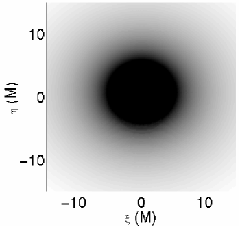
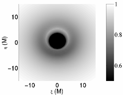
(a)	(b)
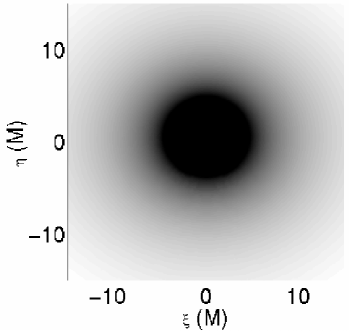
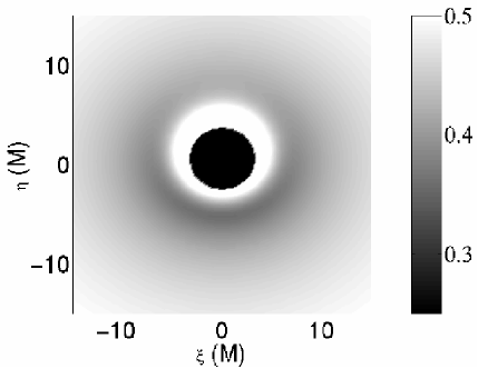
(c)	(d)

Figure 5: Shown is the normalised intensity for an optically thick, Shakura-Sunyaev disc around a Schwarzschild black hole when (a) plasma effects are neglected, (b) plasma effects are included, (c) only the left-handed circular polarisation (ordinary mode) is included, (d) only the right-handed circular polarisation (extraordinary mode) is included. Note the different scales for total intensities ((a) and (b)) and the polarised intensities ((c) and (d)). The disk is inclined $60^{\circ}$ relative to the line of sight. $\xi$ is parallel to the equatorial plane. $\eta$ is in the line of sight-azimuthal axis plane. The overall scale is set by the choice of observation frequency and the parameters of the disk and hence are not relevant here. The plasma geometry is the same as that for figures 3 and 4.

The impact that dispersive plasma effects can have upon the spectrum of an accreting object can be illustrated by maps of the intensity. Here, in addition to the plasma geometry employed in the previous two sections, an optically thick Shakura-Sunyaev disk is introduced. The emission is solely from this disk and assumed to be thermal with

$$T(r)\propto\left(1-\sqrt{R_{\mbox{\tiny min}}/r}\right)^{3/10}$$

(see e.g. Frank et al., 1992). The overall constant is dependent upon a number of disk parameters and hence is not of particular interest here. Nonetheless, it is chosen such that $kT(r=\infty)=\nu_{\mbox{\tiny obs}}$ for convenience. The innermost radius of the disk, $R_{\mbox{\tiny min}}$, is chosen to be $3M$. Doppler effects due to the rotation of the disk are ignored here.

Shown in figure 5 are the intensity maps for when (a) plasma effects are neglected, (b) plasma effects are included, (c) only the left-handed circular polarisation (ordinary mode) is considered, (d) only the right-handed circular polarisation (extraordinary mode) is considered. Because the overall flux from the disk is dependent upon the details of the accretion flow, the intensities are normalised by the highest intensity in panel (b). Comparing panels (a) and (b) demonstrates that including dispersive plasma effects makes a significant difference. This difference originates primarily from contribution by the extraordinary mode shown in panel (d).

As implied by figure 2, the shadow the black hole casts upon the extraordinary mode is less than that cast upon the ordinary mode, which is in turn less than that upon the null geodesics. In addition to the differences in the overall intensities, there is a substantial difference between the contributions from the two polarisations as seen by comparing panels (c) and (d).

4 Conclusions

The covariant magnetoionic theory developed here is distinct in many respects from the non-relativistic theory. Firstly, it qualitatively changes the topology of the dispersion relations, adding an entirely new branch, as shown in §3.1. Secondly, it allows the inclusion of gravitational lensing effects, vital for application to compact accreting objects. In addition, as shown in §3.3 and §3.4, dispersion due to plasma effects can have a significant impact upon the propagation of photons in a dense plasma environment near a black hole. As demonstrated in §3.5, this will lead to a modification of the spectrum. As a result, studies which neglect dispersive plasma effects may be inappropriate when the observation frequencies are near the plasma and/or cyclotron frequencies.

On the other hand, because plasma effects have the capability of altering the spectrum, it is possible for the underlying plasma to be observationally probed using polarised flux measurements. For example, if the horizon of the black hole in the Galactic centre can be imaged (cf. Falcke et al., 2000), observations of the polarisation map could easily distinguish the nondispersive from the dispersive case, placing limits upon the local magnetic field strength and plasma density. Integrated values for the polarisation could yield useful information about the environments of other accreting systems, such as X-ray binaries and pulsars. Because these effects can be expected to be confined to the decade in frequency surrounding the plasma frequency, they should be easily distinguishable from the effects of different accretion models.

Appendix A Geodesic Motion in the Dispersion Formalism

Given the dispersion relation in equation (73),

$$D(k_{\mu},x^{\mu})=k^{\mu}k_{\mu}-m^{2}\,,$$

and the ray equations (18),

$$\frac{dx^{\mu}}{d\tau}=\left(\frac{\partial D}{\partial k_{\mu}}\right)_{x^{\mu}}\;\;\mbox{and}\;\;\;\frac{dk_{\mu}}{d\tau}=-\left(\frac{\partial D}{\partial x^{\mu}}\right)_{k_{\mu}}\,,$$

it is possible to derive the geodesic equation. The partial derivatives on the right side of the ray equations are

$$\left(\frac{\partial D}{\partial k_{\mu}}\right)_{x^{\mu}}=2k^{\mu}\,,$$ (97)

and

$$\left(\frac{\partial D}{\partial x^{\mu}}\right)_{k_{\mu}} =\left(\frac{\partial k_{\alpha}k_{\beta}g^{\alpha\beta}}{\partial x^{\mu}}\right)_{k_{\mu}}=k_{\alpha}k_{\beta}\frac{\partial g^{\alpha\beta}}{\partial x^{\mu}}$$

$$=-k^{\alpha}k^{\beta}g_{\alpha\beta,\mu}\,.$$ (98)

Combining the ray equations gives

$$\frac{d^{2}x^{\mu}}{d\tau^{2}} =2\frac{dk^{\mu}}{d\tau}=2\frac{dk_{\nu}g^{\mu\nu}}{d\tau}$$

$$=2k_{\nu}\frac{dx^{\alpha}}{d\tau}\frac{\partial g^{\mu\nu}}{\partial x^{\alpha}}+2g^{\mu\nu}\frac{dk_{\mu}}{d\tau}$$

$$=-4k^{\beta}k^{\alpha}g^{\mu\nu}g_{\beta\nu,\alpha}+2g^{\mu\nu}k^{\alpha}k^{\beta}g_{\alpha\beta,\mu}$$

$$=-4k^{\alpha}k^{\beta}\frac{1}{2}g^{\mu\nu}\left(g_{\alpha\nu,\beta}+g_{\beta\nu,\alpha}-g_{\alpha\beta,\nu}\right)$$

$$=-\frac{dx^{\alpha}}{d\tau}\frac{dx^{\beta}}{d\tau}\Gamma^{\mu}_{\alpha\beta}\,,$$ (99)

where the definition of the Christoffel symbol was used, $\Gamma^{\mu}_{\alpha\beta}\equiv\frac{1}{2}g^{\mu\nu}\left(g_{\alpha\nu,\beta}+g_{\beta\nu,\alpha}-g_{\alpha\beta,\nu}\right)$. Collecting terms on the left produces the well known geodesic equation:

$$\frac{d^{2}x^{\mu}}{d\tau^{2}}+\frac{dx^{\alpha}}{d\tau}\frac{dx^{\beta}}{d\tau}\Gamma^{\mu}_{\alpha\beta}=0\,,$$

or

$$v^{\nu}\nabla_{\nu}v^{\mu}=0\;\;\mbox{where}\;\;v^{\mu}\equiv\frac{dx^{\mu}}{d\tau}\,.$$

References

- Agol (1997) Agol E., 1997, Ph.D. Thesis, pp 2+
- Blandford & Begelman (1999) Blandford R. D., Begelman M. C., 1999, MNRAS, 303, L1
- Boyd & Sanderson (1969) Boyd T. J. M., Sanderson J. J., 1969, Plasma Dynamics. Thomas Nelson and Sons LTD, London
- Bromley et al. (2001) Bromley B. C., Melia F., Liu S., 2001, ApJL, 555, L83
- Budden (1964) Budden K. G., 1964, Lectures on Magnetoionic Theory. Gordon and Breach, New York
- Connors et al. (1980) Connors P. A., Stark R. F., Piran T., 1980, ApJ, 235, 224
- Dendy (1990) Dendy R. O., 1990, Plasma Dynamics. Oxford University Press, Oxford
- Falcke et al. (2000) Falcke H., Melia F., Agol E., 2000, ApJL, 528, L13
- Frank et al. (1992) Frank J., King A., Raine D., 1992, Accretion Power in Astrophysics. Accretion Power in Astrophysics, ISBN 0521408636, Cambridge University Press, 1992.
- Jones & O’Dell (1977a) Jones T. W., O’Dell S. L., 1977a, ApJ, 214, 522
- Jones & O’Dell (1977b) Jones T. W., O’Dell S. L., 1977b, ApJ, 215, 236
- Krall & Trivelpiece (1973) Krall N. A., Trivelpiece A. W., 1973, Principles of plasma physics. International Student Edition - International Series in Pure and Applied Physics, Tokyo: McGraw-Hill Kogakusha, 1973
- Kulsrud & Loeb (1992) Kulsrud R., Loeb A., 1992, Phys. Rev. D, 45, 525
- Laor et al. (1990) Laor A., Netzer H., Piran T., 1990, MNRAS, 242, 560
- Lifshitz & Pitaevskii (1981) Lifshitz E. M., Pitaevskii L. P., 1981, Physical kinetics. Course of theoretical physics, Oxford: Pergamon Press, 1981
- Macquart & Melrose (2000) Macquart J.-P., Melrose D. B., 2000, ApJ, 545, 798
- Melia & Falcke (2001) Melia F., Falcke H., 2001, ARAA, 39, 309
- Misner et al. (1973) Misner C. W., Thorne K. S., Wheeler J. A., 1973, Gravitation. W.H. Freeman and Co., San Francisco
- Montgomery & Tidman (1964) Montgomery D. C., Tidman D. A., 1964, Plasma kinetic theory. McGraw-Hill Advanced Physics Monograph Series, New York: McGraw-Hill, 1964
- Narayan et al. (1998) Narayan R., Mahadevan R., Grindlay J. E., Popham R. G., Gammie C., 1998, ApJ, 492, 554
- Narayan & Yi (1994) Narayan R., Yi I., 1994, ApJL, 428, L13
- Quataert & Gruzinov (2000) Quataert E., Gruzinov A., 2000, ApJ, 539, 809
- Ruszkowski & Begelman (2002) Ruszkowski M., Begelman M. C., 2002, ApJ, 573, 485
- Sazonov (1969) Sazonov V. N., 1969, JETP, 56, 1075
- Sazonov & Tsytovich (1968) Sazonov V. N., Tsytovich V. N., 1968, Radiofizika, 11, 1287
- Thompson et al. (1994) Thompson C., Blandford R. D., Evans C. R., Phinney E. S., 1994, ApJ, 422, 304
- Weinberg (1962) Weinberg S., 1962, Physical Review, 126, 1899