Abundance of damped Lyman-$\alpha$ absorbers in cosmological SPH simulations

Abstract

We use cosmological smoothed-particle hydrodynamics (SPH) simulations of the $\Lambda$ cold dark matter (CDM) model to study the abundance of damped Lyman-$\alpha$ absorbers (DLAs) in the redshift range $z=0-4.5$. We compute the cumulative DLA abundance by using the relation between DLA cross-section and the total halo mass inferred from the simulations. Our approach includes standard radiative cooling and heating with a uniform UV background, star formation, supernova feedback, as well as a phenomenological model for feedback by galactic winds. The latter allows us to examine, in particular, the effect of galactic outflows on the abundance of DLAs. We employ the “conservative entropy” formulation of SPH developed by Springel & Hernquist (2002), which mitigates against the systematic overcooling that affected earlier simulations. In addition, we utilise a series of simulations of varying box-size and particle number to isolate the impact of numerical resolution on our results.

We show that the DLA abundance was overestimated in previous studies for three reasons: (1) the overcooling of gas occurring with non-conservative formulations of SPH, (2) a lack of numerical resolution, and (3) an inadequate treatment of feedback. Our new results for the total neutral hydrogen mass density, DLA abundance, and column density distribution function all agree reasonably well with observational estimates at redshift $z=3$, indicating that DLAs arise naturally from radiatively cooled gas in dark matter haloes that form in a $\Lambda$CDM universe. Our simulations suggest a moderate decrease in DLA abundance by roughly a factor of two from $z=4.5$ to 3, consistent with observations. A significant decline in abundance from $z=3$ to $z=1$, followed by weak evolution from $z=1$ to $z=0$, is also indicated, but our low-redshift results need to be interpreted with caution because they are based on coarser simulations than the ones employed at high redshift. Our highest resolution simulation also suggests that the halo mass-scale below which DLAs do not exist is slightly above $10^{8}\,h^{-1}{\rm M_{\odot}}$ at $z=3-4$, somewhat lower than previously estimated.

1 Introduction

Damped Lyman-$\alpha$ absorbers, historically defined as quasar absorption systems with neutral hydrogen column density ${N_{\rm HI}}>2\times 10^{20}\rm cm^{-2}$ (Wolfe et al., 1986), are one of the best probes of structure formation in the early universe. Since DLAs are dense concentrations of gas often found at $z\geq 3$, it is natural to suppose that they are closely linked to the formation of galaxies and stars at high redshift. It has become clear in recent years from the study of Lyman-break galaxies at $z\sim 3-4$ (e.g. Adelberger et al., 1998; Steidel et al., 1999; Shapley et al., 2001) that the assembly of galaxies is actively going on at $z\sim 3$, consistent with hierarchical structure formation in a cold dark matter universe (e.g. Mo & Fukugita, 1996; Baugh et al., 1998; Jing & Suto, 1998; Katz, Hernquist & Weinberg, 1999; Kauffmann et al., 1999; Mo, Mao, & White, 1999; Nagamine, 2002; Weinberg, Hernquist & Katz, 2002).

A picture of the history of cosmic star formation emerging from both theory and observation is that it rises from the present towards high redshift, even beyond $z=3$ (e.g. Pascarelle, Lanzetta, & Fernández-Soto, 1998; Blain et al., 1999; Nagamine et al., 2001a; Lanzetta et al., 2002; Springel & Hernquist, 2003b; Hernquist & Springel, 2002). The conversion of gas into stars is, therefore, taking place at a significant rate at $z\geq 3$. If DLAs dominate the neutral hydrogen gas content of the Universe at $z\sim 3$, they are thus serving as an important reservoir of neutral gas for star formation. Determining the physical nature and number density of DLAs may hence be one of the most important keys for further constraining the cosmic star formation history and theories of galaxy formation.

Although the current sample of observed DLAs at $z\geq 1.5$ is not yet as large as that of Lyman-break galaxies (where $\approx 1000$ are known), the total number of DLAs that have been discovered is now approaching $\approx 100$, and the number density per unit redshift of high column density systems appears to peak at around $z\sim 3$ (Storrie-Lombardi & Wolfe, 2000). At lower redshift, the situation is rather different. The identification of DLAs at $z<1.5$ has been difficult because they are rare and the need for ultra-violet (UV) spectroscopy to detect Ly$\alpha$ absorption at these low redshifts. The number of quasars studied in UV has been small until recently. To overcome this difficulty, Rao & Turnshek (2000) searched for DLAs in 87 Mg ii absorbers, and uncovered 12 new systems. There are 23 DLAs at $z<1.65$ listed by Rao & Turnshek (2000).

Despite the likely importance of DLAs and the accumulation of observational data on them, their true nature remains controversial. Historically, it has often been suggested that high-redshift DLAs are large, rapidly rotating discs, because DLAs have properties similar to local galactic discs, such as large neutral hydrogen column densities together with low degrees of ionisation and small velocity dispersions (Wolfe et al., 1986). More recently, Prochaska & Wolfe (1997, 1998) argued that the observed distribution of velocity widths and the asymmetric absorption profiles of low-ionisation ionic species can be best described by massive, rapidly rotating cold discs.

On the other hand, Haehnelt, Steinmetz, & Rauch (1998) examined a small number of dark matter haloes in a high-resolution (sub-kpc) SPH simulation, and showed that such observational signatures can also be explained by a mixture of rotation, random motions, infall, and mergers of protogalactic clumps. There are some observational indications (Le Brun et al., 1997; Rao & Turnshek, 1998; Kulkarni et al., 2000, 2001) from direct imaging studies that luminous disc galaxies may not represent the dominant population of DLA galaxies (i.e. galaxies that host DLAs). Although the possibility of artifacts due to point-spread-function effects cannot be fully excluded, these observations suggest that some DLA galaxies could be compact, clumpy objects, or low surface brightness galaxies, rather than large, well-formed protogalactic disks or spheroids.

Robust numerical estimates of DLA properties have been hampered by the significant requirements on numerical resolution needed to capture the full population of DLAs. Earlier studies by Katz et al. (1996) and Hernquist et al. (1996) showed that the observed Hi  column density distribution can be reproduced within a factor of a few in hydrodynamic simulations based on a CDM model over a wide range of column densities $10^{14}\rm cm^{-2}\leq{N_{\rm HI}}\leq 10^{22}\rm cm^{-2}$. Their results demonstrated that the Ly-$\alpha$ forest develops naturally in the hierarchical clustering scenario of CDM universes, and that DLAs and Lyman-limit systems (${N_{\rm HI}}\geq 10^{17}\rm cm^{-2}$) arise in these models from radiatively cooled gas inside dark matter haloes that host forming galaxies at high redshift. However, their calculations were based on simulations of a critical-density universe with $\Omega_{\rm m}=1$, and could not resolve haloes with masses $M<10^{11}\,h^{-1}{\rm M_{\odot}}$.

Subsequently, Gardner et al. (1997a, b, 2001) extended the earlier results of Katz et al. (1996) and Hernquist et al. (1996) by developing a method to correct for the resolution limitations of the simulations. They measured the relation between absorption cross-section and halo circular velocity from hydrodynamic simulations, and then convolved it with the analytic halo mass function (e.g. Press & Schechter, 1974; Sheth & Tormen, 1999) to compute the cumulative abundance of DLAs. Using this correction method, they were able to reproduce the observed abundance of DLAs if they required that haloes with circular velocity $v_{c}\leq 60\,\rm km\,s^{-1}$ (which corresponds to $M\approx 2\times 10^{10}\,h^{-1}{\rm M_{\odot}}$) did not harbour DLAs. However, their simulations could not resolve haloes with masses below $10^{10}\,h^{-1}{\rm M_{\odot}}$, although such haloes may still host a significant number of DLAs. If the absorption cross-section of haloes with $M<10^{10}\,h^{-1}{\rm M_{\odot}}$ does not follow the same relation between the cross-section and the halo mass as determined from higher mass haloes, the DLA abundance could be either over- or underestimated. Simulations of higher resolution are hence clearly needed to make more robust predictions for the DLA abundance at redshift $z=3$.

Recently, Springel & Hernquist (2002) developed a novel formulation of SPH that is based on integrating the entropy as an independent thermodynamic variable (e.g. Lucy, 1977; Hernquist, 1993), and which takes variations of the SPH smoothing lengths self-consistently into account. They showed that this new version maintains contact discontinuities (as they arise at the interface between cold and hot gas in haloes) much better than previous treatments of SPH. Consequently, their formulation does not suffer from the severe overcooling that was typically seen in previous SPH simulations. We hence use this new methodology for our studies of DLAs.

Run	Boxsize	${N_{\rm p}}$	$m_{\rm DM}$	$m_{\rm gas}$	$\epsilon$	$z_{\rm end}$	wind
R3	3.375	$2\times 144^{3}$	$9.29\times 10^{5}$	$1.43\times 10^{5}$	0.94	4.00	strong
R4	3.375	$2\times 216^{3}$	$2.75\times 10^{5}$	$4.24\times 10^{4}$	0.63	4.00	strong
O3	10.00	$2\times 144^{3}$	$2.42\times 10^{7}$	$3.72\times 10^{6}$	2.78	2.75	none
P3	10.00	$2\times 144^{3}$	$2.42\times 10^{7}$	$3.72\times 10^{6}$	2.78	2.75	weak
Q3	10.00	$2\times 144^{3}$	$2.42\times 10^{7}$	$3.72\times 10^{6}$	2.78	2.75	strong
Q4	10.00	$2\times 216^{3}$	$7.16\times 10^{6}$	$1.10\times 10^{6}$	1.85	2.75	strong
Q5	10.00	$2\times 324^{3}$	$2.12\times 10^{6}$	$3.26\times 10^{5}$	1.23	2.75	strong
D4	33.75	$2\times 216^{3}$	$2.75\times 10^{8}$	$4.24\times 10^{7}$	6.25	1.00	strong
D5	33.75	$2\times 324^{3}$	$8.15\times 10^{7}$	$1.26\times 10^{7}$	4.17	1.00	strong
G4	100.0	$2\times 216^{3}$	$7.16\times 10^{9}$	$1.10\times 10^{9}$	12.0	0.00	strong
G5	100.0	$2\times 324^{3}$	$2.12\times 10^{9}$	$3.26\times 10^{8}$	8.00	0.00	strong

Table 1: Simulations employed in this study. The box-size is given in units of $h^{-1}{\rm\,Mpc}$, ${N_{\rm p}}$ is the particle number of dark matter and gas (hence $\times\,2$), $m_{\rm DM}$ and $m_{\rm gas}$ are the masses of dark matter and gas particles in units of $\,h^{-1}{\rm M_{\odot}}$, respectively, $\epsilon$ is the comoving gravitational softening length in units of $h^{-1}{\rm\,kpc}$, and $z_{\rm end}$ is the ending redshift of the simulation. The value of $\epsilon$ is a measure of spatial resolution. From the top to the bottom row, we refer to R3 & R4 collectively as ‘R-series’, the next 5 runs (O3 to Q5) are called ‘Q-series’, D4 & D5 are called ‘D-series’, and G4 & G5 are called ‘G-series’. The ‘strong-wind’ simulations form a subset of the runs analysed by Springel & Hernquist (2003b).

Our simulations also include a novel method for treating star formation and feedback, as proposed by Springel & Hernquist (2003a). It is based on a sub-resolution multi-phase description of the dense, star-forming interstellar medium (ISM) and a phenomenological model for strong feedback by galactic winds. The inclusion of winds was motivated by the possibility that outflows from galaxies at high redshift (Pettini et al., 2002) play a role in distributing metals into the intergalactic medium (e.g. Aguirre et al., 2001a, b), and they may also alter the distribution of neutral gas around galaxies (Adelberger et al., 2002), although this process remains uncertain (e.g. Croft et al., 2002; Kollmeier et al., 2003). Together with the increase in numerical resolution provided by our simulations, it is of interest to see how refinements in physical modelling modify the predictions of DLA properties in a CDM universe.

In this paper, we focus on the abundance of DLAs in the redshift range $z=0-4.5$. The present work extends and complements earlier numerical work by Katz et al. (1996) and Gardner et al. (2001). Physical properties of DLAs such as their star formation rates, metallicities, and their relation to galaxies will be presented elsewhere.

The paper is organised as follows. In Section 2, we briefly describe the numerical parameters of our simulation set. We then present the evolution of the total neutral hydrogen mass density in the simulations in Section 3. In Section 4, we describe how we compute the Hi  column density and DLA cross-section as a function of total halo mass. In Section 5, we determine the cumulative abundance of DLAs, and discuss the evolution of DLA abundance from $z=4.5$ to $z=0$. The Hi  column density distribution function is presented in Section 6. Finally, we summarise and discuss the implication of our work in Section 7.

2 Simulations

We analyse a large set of cosmological SPH simulations that differ in box size, mass resolution and feedback strength, as summarised in Table 1. In particular, we consider box sizes ranging from 3.375 to $100\,h^{-1}{\rm Mpc}$ on a side, with particle numbers between $2\times 144^{3}$ and $2\times 324^{3}$, allowing us to probe gaseous mass resolutions in the range $4.2\times 10^{4}$ to $1.1\times 10^{9}\,h^{-1}{\rm M}_{\odot}$. These simulations are partly taken from a study of the cosmic star formation history by Springel & Hernquist (2003b), supplemented by additional runs with weaker or no galactic winds. The joint analysis of this series of simulations allows us to significantly broaden the range of spatial and mass-scales that we can probe compared to what is presently attainable within a single simulation.

There are three main new features to our simulations. First, we use a new “conservative entropy” formulation of SPH (Springel & Hernquist, 2002) which explicitly conserves entropy (in regions without shocks), as well as momentum and energy, even when one allows for fully adaptive smoothing lengths. This formulation moderates the overcooling problem present in earlier formulations of SPH (see also Yoshida et al., 2002; Pearce et al., 1999; Croft et al., 2001).

Second, highly over-dense gas particles are treated with an effective sub-resolution model for the ISM, as described by Springel & Hernquist (2003a). In this model, the dense ISM is pictured to be a two-phase fluid consisting of cold clouds in pressure equilibrium with a hot ambient phase. Each gas particle represents a statistical mixture of these phases. Cold clouds grow by radiative cooling out of the hot medium, and this material forms the reservoir of baryons available for star formation. Once star formation occurs, the resulting supernova explosions deposit energy into the hot gas, heating it, and also evaporate cold clouds, transferring cold gas back into the ambient phase. This establishes a tight self-regulation mechanism for star formation in the ISM.

Third, we implemented a phenomenological model for galactic winds in order to study the effect of outflows on DLAs, galaxies, and the intergalactic medium (IGM). In this model, gas particles are stochastically driven out of the dense star-forming medium by assigning an extra momentum in random directions, with a rate and magnitude chosen to reproduce mass-loads and wind speeds similar to those observed. See Springel & Hernquist (2003a) for a detailed discussion of this method.

Most of our simulations employ a “strong” wind of speed $484\,{\rm km\,s^{-1}}$, but for the $10\,h^{-1}{\rm Mpc}$ box (runs O3, P3, Q3, Q4, Q5; collectively called ‘Q-series’) we also varied the wind strength. Therefore, this Q-series can be used to study both the effect of numerical resolution and the consequences of feedback from galactic winds. The runs in the other simulation series then allow the extension of the strong wind results to smaller scales (‘R-Series’), or to larger box-sizes and hence lower redshift (‘D-’ and ‘G-Series’). Our naming convention is such that runs of the same model (box-size and included physics) are designated with the same letter, with an additional number specifying the particle resolution.

Our calculations include a uniform UV background radiation field of a modified Haardt & Madau (1996) spectrum, where reionisation takes place at $z\simeq 6$ (see Davé et al., 1999), as suggested by observations (e.g. Becker et al., 2001) and radiative transfer calculations of the impact of the stellar sources in our simulations on the IGM (e.g. Sokasian et al., 2003). The radiative cooling and heating rate is computed as described by Katz et al. (1996) assuming that the gas is optically thin and in ionization equilibrium. The abundance of different ionic species, including H⁰, He⁰, H⁺, He⁺, and He⁺⁺, is computed by solving the network of equilibrium equations self-consistently with a specified UV background radiation. The results presented in this paper should not be affected by the assumption of ionization equilibrium as we are dealing with high density regions where this assumption is satisfied well. The adopted cosmological parameters of all runs are $(\Omega_{\rm m},\Omega_{\Lambda},\Omega_{\rm b},\sigma_{8},h)=(0.3,0.7,0.04,0.9,0.7)$. The simulations were performed on the Athlon-MP cluster at the Center for Parallel Astrophysical Computing (CPAC) at the Harvard-Smithsonian Center for Astrophysics, using a modified version of the parallel GADGET code (Springel, Yoshida & White, 2001).

3 Neutral Hydrogen Mass Density

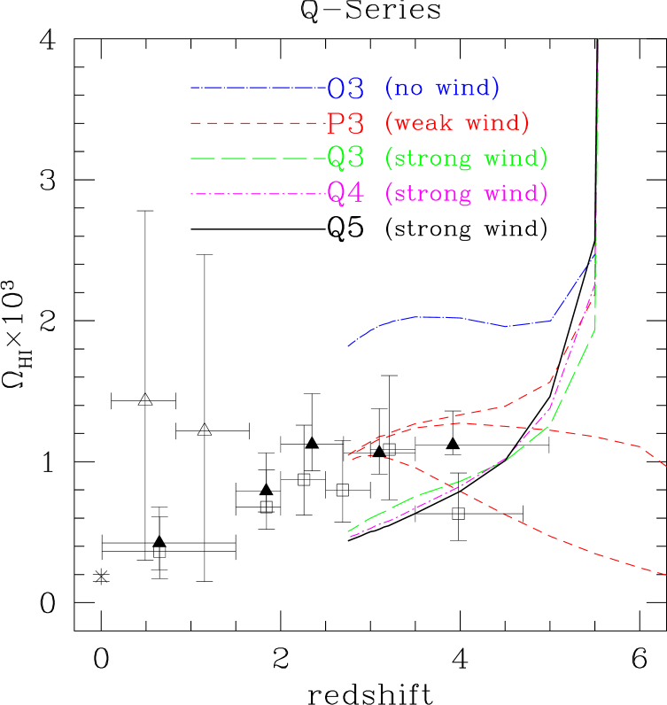
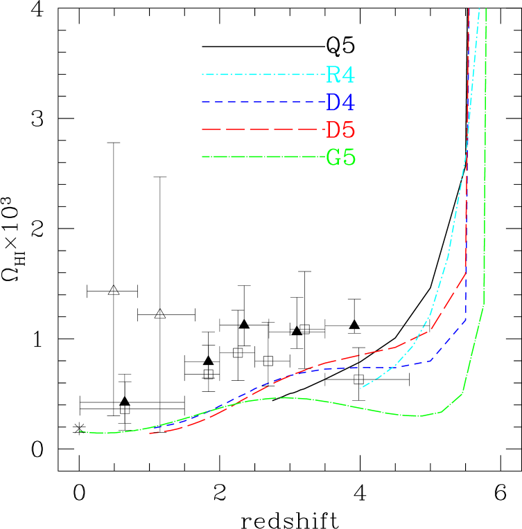
Figure 1: Evolution of the total neutral hydrogen mass density in each simulation box as a function of redshift. The plotted values are $\Omega_{\rm HI}\times 10^{3}$. We also show observational data points from Storrie-Lombardi & Wolfe (2000, open squares; only for DLAs), Péroux et al. (2001, filled triangles; including the correction for the neutral gas not included in DLAs), Rao & Turnshek (2000, open triangles), and Zwaan et al. (1997, open cross at $z=0$). Left panel: A comparison of the Q-series (runs in $10\,h^{-1}{\rm Mpc}$ boxes) is shown. The decrease in $\Omega_{\rm HI}$ from O3 (no wind) to P3 (weak wind), and then to Q3 (strong wind), shows the effect of feedback by galactic winds. The comparison between Q3, Q4, and Q5 shows the level of convergence achieved for runs with different resolution. For P3 (top short-dashed line), we separately show $\Omega_{\rm HI}$ in regions of overdensity $1+\delta>10^{3}$ and $10^{4}$ (middle and bottom short-dashed line, respectively). Right panel: Results for the R-, D-, and G-series are shown. Q5 is also included to ease comparison with the left panel. Results for R3 and G4 are omitted for clarity (see text).

In our simulation methodology, gas is subject to a thermal instability yielding a multiphase medium once the physical gas density lies above a threshold density $\rho_{\rm th}$, which marks the onset of cold cloud formation. If the physical density is lower than this threshold, a particle represents ordinary gas in a single phase. In this latter case, the neutral hydrogen mass of the particle can be computed as follows:

$$m_{\rm HI}=N_{\rm h}\cdot X_{\rm H}\cdot m_{\rm gas}\quad(\rho<\rho_{\rm th}),$$ (1)

where $X_{\rm H}=0.76$ is the primordial mass fraction of hydrogen, and $N_{\rm h}$ is the number density of neutral hydrogen atoms in units of the total number density of hydrogen nuclei. The quantity $N_{\rm h}$ is computed by solving the ionisation balance as a function of density and current UV background flux.

If the gas density is higher than the threshold density, we identify the mass of neutral gas with the mass of cold clouds contained in the multiphase medium. The mass of neutral hydrogen of such a multiphase particle is then given by

$$m_{\rm HI}=x\cdot X_{\rm H}\cdot m_{\rm gas}\quad(\rho>\rho_{\rm th}),$$ (2)

where $x$ is the mass fraction of cold clouds. In the multiphase model of Springel & Hernquist (2002b), $x$ can be computed as

$$x\equiv\rho_{c}/\rho=1+\frac{1}{2y}-\sqrt{\frac{1}{y}+\frac{1}{4y^{2}}},$$ (3)

where the quantities $y$ and $\rho_{\rm th}$ are defined by

$$y\equiv\frac{t_{*}\Lambda_{\rm net}(\rho,u_{h})}{\rho[\beta u_{\rm SN}-(1-\beta)u_{c}]}$$ (4)

and

$$\rho_{\rm th}=\frac{x_{\rm th}}{(1-x_{\rm th})^{2}}\frac{\beta u_{\rm SN}-(1-\beta)u_{c}}{t_{*}^{0}\Lambda(u_{\rm SN}/A_{0})}.$$ (5)

Here, $\Lambda_{\rm net}(\rho,u)$ is the usual cooling function, and we have defined $\Lambda(\rho,u)\equiv\Lambda_{\rm net}(\rho,u)/\rho^{2}$. The parameter $\beta$ gives the mass fraction of short-lived stars that explode as supernovae, $u_{\rm SN}$ describes the energy released by the supernovae, $u_{c}$ is the assumed temperature of the cold clouds, $u_{h}$ the temperature of the hot medium, $A_{0}$ the cloud evaporation parameter, and $t_{*}^{0}$ gives the star formation time-scale. The quantity $x_{\rm th}=(u_{h}-u_{4})/(u_{h}-u_{c})\simeq 1-A_{0}u_{4}/u_{\rm SN}$ is the mass fraction in cold clouds at the threshold density, where $u_{4}$ is the specific energy corresponding to $T=10^{4}~{}{\rm K}$. We refer to Springel & Hernquist (2002b) for a more detailed explanation of these parameters, and a derivation of equations (3) to (5).

In Figure 1, we show the total neutral hydrogen mass density as a function of redshift. The values plotted are given in terms of $\Omega_{\rm HI}\times 10^{3}$. At redshifts above six, essentially all the hydrogen in the simulation box is still neutral ($\Omega_{\rm HI}\simeq X_{\rm H}\Omega_{\rm b}=0.0304$). Once the ionising background sets in at $z=6$, the neutral hydrogen starts to become ionised and the neutral fraction decreases rapidly by a few orders of magnitude; i.e. reionisation takes place. Note that with the exception of the R-Series, our earliest simulation output at $z<6$ corresponds to $z=5.5$. This is why most of the models in Figure 1 seem to show a rapid rise of $\Omega_{\rm HI}$ already at $z=5.5$, which simply arises by drawing a line to the data point at $z=6$ which lies a few orders of magnitude higher in this linear plot.

We also include observational data points, for comparison. The data points from Storrie-Lombardi & Wolfe (2000, open squares) account only for DLAs, but those of Péroux et al. (2001, filled triangles) include a correction for the neutral gas that is in sub-DLAs $(10^{19}<{N_{\rm HI}}<10^{20}\rm cm^{-2}$). Data points from Rao & Turnshek (2000, solid triangles) at low-redshift and Zwaan et al. (1997, open cross) at $z=0$ are also shown.

In the left panel of Figure 1, we compare results only for the Q-series ($10\,h^{-1}{\rm Mpc}$ box), allowing us to assess convergence as a function of mass resolution and to investigate the dependence of the results on the strength of feedback from winds.

The comparison between Q3, Q4, and Q5 (strong wind) shows that there is quite good agreement between runs with different numerical resolution. In fact, the results for Q3, Q4, and Q5 are essentially identical at $z\simeq 4.5$, with Q5 being slightly higher for $z\geq 4.5$ than its lower resolution counterparts, while for $z\leq 4.5$ the opposite trend is observed. This mild effect can be understood as follows: in a higher resolution run like Q5, many more small dark matter haloes can be resolved than in a lower resolution run (like Q3), particularly at early times, where gas can cool very efficiently. As a result, the higher resolution simulation develops a larger fraction of cold and hence neutral gas at high redshift. However, an increased fraction of cold gas will also trigger more intense star formation that both consumes neutral gas and leads to gas ejection by winds from low mass haloes. Subsequently, the neutral fraction can then fall slightly below the lower resolution runs.

Comparing the results for the models O3 (no wind), P3 (weak wind), and Q3 (strong wind) shows the impact of feedback by galactic winds. As the wind strength increases, the neutral density $\Omega_{\rm HI}$ decreases. More neutral gas is then ejected out of the dense ISM into the intergalactic medium, where it becomes highly ionised by UV background radiation. Interestingly, ‘O3’ (no wind run) exceeds all observed data points, so a feedback effect such as galactic winds appears necessary to make the $\Omega_{\rm HI}$ measurements of the simulations consistent with observations. The results for our ‘strong-wind’ runs (Q3, Q4, Q5) underpredict the observational estimates at $z=3$ slightly, but there is still marginal agreement within $1\,\sigma$, which is encouraging. However, the best value for the galactic wind strength parameter for our simulation seems to lie somewhere between that of P3 (weak wind) and the Q-runs (strong wind).

For the ‘P3’ run, we also show separate measurements of $\Omega_{\rm HI}$ restricted to regions of overdensity $1+\delta>10^{3}$ and $10^{4}$, respectively (red short-dashed lines). The fact that the lines for $1+\delta>10^{4}$ and $10^{3}$ have converged by $z\simeq 3$ shows that most of the neutral hydrogen mass in the universe is already in a highly concentrated form by this epoch.

In the right panel of Figure 1, we show our results for simulations of the R-, D-, and G-series, together with Q5 for reference to the left panel. The results for D4 and D5 are consistent with one another at $z=3$. ‘R3’ is not shown because it is almost identical to ‘R4’, and ‘G4’ is omitted because it underpredicts $\Omega_{\rm HI}$ significantly due to lack of resolution at $z\geq 3$. By comparing to the simulations of the Q- and D-series, we see that the resolution of the G-series is not sufficient to correctly describe the neutral fraction at $z=3$. This is because even the $2\times 324^{3}$ run G5 misses the neutral gas content in large numbers of small dark matter haloes that are present in the higher resolution runs at $z=3$, such as those of the Q-series. Therefore, we consider Q5 to be the most reliable run at $z=3$ among our simulation set. We also see that $\Omega_{\rm HI}$ of ‘R4’ is lower than that of ‘Q5’, despite the fact that the R-series has higher mass resolution than the Q-series. This is likely due to the rather small box-size of the R-series compared to the Q-series, which leads to an insufficient sampling of rare, massive objects, and compromises the use of R4 as a truly representative sample of the universe.

The effect of the multiphase model adopted in the current simulations can be assessed by setting the value of cold gas mass fraction to $x=1$ for the multiphase gas particles [see Equation (3)]. We find that the value of $\Omega_{\rm HI}$ becomes larger by about 15% in such a case. This suggests that previous formulations of hydrodynamic simulations without a consideration for the multiphase nature of the gas would have overestimated the cold gas fraction by a similar amount.

4 Hi  Column Density & DLA Cross-Section

We now describe how we compute the Hi  column density ${N_{\rm HI}}$ and the DLA cross-section $\sigma_{\rm DLA}$ for each dark matter halo. First, we identify dark matter haloes by applying a conventional friends-of-friends algorithm to the dark matter particles in each simulation. We set the minimum number of dark matter particles for a halo to 32; i.e. haloes with fewer particles are not included in the group catalogue. We have confirmed that the dark matter halo mass functions agree well with the analytic mass function of Sheth & Tormen (1999). After dark matter haloes are identified, we associate each gas and star particle with their nearest dark matter particle, including them in the particle list of the corresponding haloes, when appropriate.

Then, for each halo, a uniform grid covering the entire halo and whose grid-size is equal to the gravitational softening length, is placed at the center-of-mass of the halo. We then project the neutral gas in the halo onto a plane, and obtain the column density of each grid-cell in this plane. The neutral mass of each gas particle is smoothed over a spherical region of grid-cells, weighted by the SPH kernel. To check the robustness of the result, we also tried a cloud-in-cell assignment scheme where the neutral mass of each gas particle is uniformly distributed over a cubic region of size $\ell=(\frac{4\pi}{3})^{1/3}s$ and $\frac{1}{2}(\frac{4\pi}{3})^{1/3}s$ centered on the particle. Here $s$ is the SPH smoothing length. Differences in the smoothing method can lead to slight differences in the Hi  column density distribution, as we will discuss later in Figure 7. In the following, we adopt the SPH smoothing method for our primary results unless explicitly stated otherwise.

Once the comoving neutral mass density $\rho_{i,\rm HI}$ in each grid-cell of volume $\epsilon^{3}$ is known, it is straightforward to project the density distribution along the direction perpendicular to the plane to obtain the column density as

$${N_{\rm HI}}=\sum_{i}\rho_{i,{{\rm HI}}}\cdot\epsilon/m_{p}\cdot(1+z)^{2},$$ (6)

where $\epsilon$ is the comoving gravitational softening length, $m_{p}$ is the proton mass, and $z$ is the redshift.

Note that in the present study, we do not apply a self-shielding correction when computing the neutral hydrogen fraction. As Katz et al. (1996) have shown, damped systems with column densities above ${N_{\rm HI}}\simeq 10^{20}\rm cm^{-2}$ are essentially fully neutral and are not affected by self-shielding. The correction is expected to be large for systems with $10^{17}\leq{N_{\rm HI}}\leq 10^{20}\rm cm^{-2}$, however. A full 3-dimensional treatment of self-shielding is beyond the scope of the present study, but it is clearly an interesting and important issue in its own right. The results presented in this paper for very high column density systems should however be robust against self-shielding corrections.

Once the column density of each cell in the projected plane is obtained, we estimate the comoving DLA cross-section of each halo by simply counting the number of grid-cells that exceed ${N_{\rm HI}}=2\times 10^{20}\rm cm^{-2}$ and multiplying this number by the comoving unit area $\epsilon^{2}$ of the grid-cells.

4.1 DLA cross-section at redshift 3

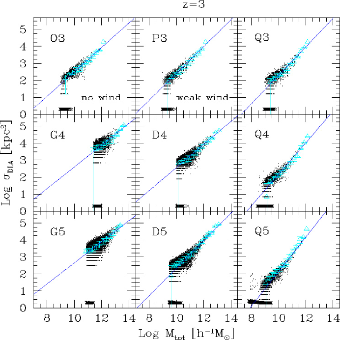
Figure 2: Comoving DLA cross-section $\sigma_{\rm DLA}$ as a function of total halo mass at $z=3$ for the Q-, D-, and G-series. All panels are for runs with ‘strong winds’, except where labelled otherwise. We show median values for logarithmic mass bins as open triangles, and the quartiles in each bin are indicated in the form of error bars. The horizontal concentration of crosses at $\log\sigma_{\rm DLA}=0.3$ indicates haloes without DLAs. The solid lines are power-law fits to the median points as described in the text.

In Figure 2, we show the comoving DLA cross-section $\sigma_{\rm DLA}$ as a function of total halo mass ${M_{\rm tot}}$ at redshift $z=3$. All panels are for runs that include ‘strong winds’, except where explicitly labeled otherwise. The data points are binned in terms of $\log{M_{\rm tot}}$, and the median value in each bin is shown by the open triangles. The quartiles in each mass bin are shown as error bars. For plotting purposes only, we assign an arbitrary value of $\log\sigma_{\rm DLA}=0.3$ to all haloes with no DLAs, and they are shown by the crosses at the bottom of each panel. We included these ‘no-DLA haloes’ in computing the median cross-section, therefore the error bars in the lowest mass-bins sometimes extend to the bottom of the figure.

We then fit the median points to a power law, $\sigma_{\rm DLA}\propto{M_{\rm tot}}^{\alpha}$, assuming a functional form of

$$\log\sigma_{\rm DLA}=\alpha(\log{M_{\rm tot}}-12)+\beta,$$ (7)

and determine the values of the slope ‘$\alpha$’ and the normalisation ‘$\beta$’ by least-squares fitting. The value of $\beta$ hence gives the value of $\log\sigma_{\rm DLA}$ at ${M_{\rm tot}}=10^{12}\,h^{-1}{\rm M_{\odot}}$. We chose this reference mass-scale because it is well covered by most of the simulations used in this paper.

Unlike the analysis of Gardner et al. (1997a), we do not invoke a limiting halo mass below which a dark matter halo does not harbour a DLA. As can be seen in all the panels of Figure 2, such a clear cutoff does not really exist, and DLAs continue to be found in haloes with masses down to ${M_{\rm tot}}\simeq 10^{8.3}\,h^{-1}{\rm M_{\odot}}$ in ‘Q5’. We will come back to this point later.

Redshift 3

Run	slope $\alpha$	$\beta$
O3	0.72	3.94
P3	0.79	3.99
Q3	0.84	3.98
Q4	0.93	4.03
Q5	1.02	4.18
D4	0.68	3.93
D5	0.81	3.96
G4	0.64	3.88
G5	0.62	3.89

Table 2: The parameters obtained by least-square fitting the power-law of equation (7) to the median points shown in Figure 2.

We summarise the results of our power-law fitting in Table 2. It is satisfying that the values of the normalisation ‘$\beta$’ agree very well among different runs. This demonstrates that our results for runs with widely varying resolution are numerically well-converged at the mass-scale of ${M_{\rm tot}}=10^{12}\,h^{-1}{\rm M_{\odot}}$. It is seen that the slope ‘$\alpha$’ becomes steeper as the galactic wind strength increases from O3 to P3, and further to Q3. This is because gas in low-mass haloes is lost at a higher rate in runs with stronger winds, making the DLA cross-sections decrease for small haloes. Another trend seen in Table 2 is that the slope becomes somewhat steeper as the resolution of the simulation increases from Q3 to Q4, and then to Q5. This can be explained by the fact that higher resolution simulations can resolve star formation in small haloes, leading to ejection of gas out of them, lowering their content of neutral gas. On the other hand, a lower resolution simulation misses this star formation, resulting in an overestimate of the baryon and neutral fraction in the first generation of haloes that is ‘seen’ in the simulation.

Gardner et al. (2001) reported a slightly shallower slope even compared to ‘O3’ (no-wind run): $\sigma_{\rm DLA}\propto v_{c}^{1.57}\propto M^{0.52}$ (see Table 2 of their paper). Here, $v_{c}$ is the circular velocity of a halo, related to the halo mass by $v_{c}\propto{M}^{1/3}$. A shallower slope in general implies a higher abundance of DLAs. A number of effects are responsible for this difference: (1) Their resolution was slightly lower (${N}=128^{3}$) than that of our O3/P3/Q3-runs. (2) The overcooling problem in previous formulations of SPH may have caused the slope to be shallower owing to an overestimate of the neutral gas fraction, particularly in small haloes. With our new ‘conservative entropy’ formulation of SPH, the cold gas fraction in haloes is expected to be lower, although the magnitude of this effect as a function of halo mass is not fully clear. (3) Their treatment of feedback is known to be inefficient, because thermal energy injected into the gas is radiated away very rapidly. However, given that our ‘O3’-run overpredicts $\Omega_{\rm HI}$ (Figure 1) at $z=3$, some form of strong feedback seems necessary to provide agreement with the observations. Noting that the slope of the power-law fit steepens as the wind strength and resolution increase, we hence conclude that the slope of Gardner et al. (2001) was probably too shallow. This conclusion will be strengthened when we discuss the abundance of DLAs in Section 5 and the column-density distribution function in Section 6.

4.2 DLA cross-section at redshift 4.5

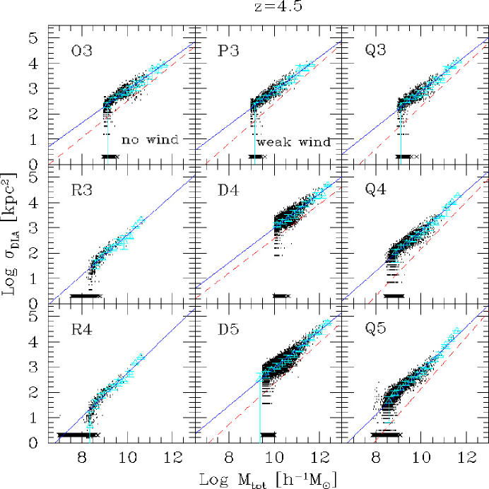
Figure 3: Same as Figure 2, but for $z=4.5$. Here, instead of G4 and G5, we show results for R3 and R4. The solid slanted lines are the best-fits to the median points (indicated by the open triangles) with a power-law (equation 7), and the short-dashed lines are the fits we obtained at $z=3$, for comparison. The horizontal concentration of crosses at $\log\sigma_{\rm DLA}=0.3$ indicates haloes that do not harbour a DLA. Note that the range along the x-axis is different from that of Figure 2.

Redshift 4.5

Run	slope $\alpha$	$\beta$
R3	0.79	4.29
R4	0.86	4.46
O3	0.64	4.21
P3	0.67	4.24
Q3	0.71	4.31
Q4	0.79	4.44
Q5	0.87	4.59
D4	0.68	4.34
D5	0.74	4.42
G4	0.56	4.31
G5	0.65	4.30

Table 3: The parameters obtained by least-squares fitting the power-law of equation (7) to the median points shown in Figure 3.

In Figure 3, we show the DLA cross-section at $z=4.5$ as a function of total halo mass. As before, the solid lines show power-law fits that were obtained as described in the previous subsection, while the short-dashed lines are the fits at redshift $z=3$, for comparison. Note that we do not plot results for the G-series but instead show the R-series, which has much higher resolution, but was evolved only to $z=4$ due to its small box-size. The results of the power-law fitting are summarised in Table 3. Similar to $z=3$, the values of the normalisation ‘$\beta$’ agree very well with each other between runs of differing resolution. The generic trends in the slope as a function of wind strength and resolution are also similar to what we saw for $z=3$.

At the low-mass end of runs R3 and R4, we see that the DLA cross-section is dropping prominently at ${M_{\rm tot}}\sim 10^{8.3}\,h^{-1}{\rm M_{\odot}}$, strongly departing from the fitted power-law. To avoid being affected by this turn-down, we do not use the median points below $\log\sigma_{\rm DLA}=1.0$ for our power-law fitting. A similar feature is seen in Q4 and Q5 at the same mass-scale. Note that the resolution of the R-series is sufficient to resolve haloes with ${M_{\rm tot}}=10^{8}\,h^{-1}{\rm M_{\odot}}$ quite well, so this downturn in DLA cross-section is unlikely to be a resolution artifact. Instead, it is probably due to the physical effect that the gas in these haloes is easily photoevaporated by the ionising background, and/or ejected from haloes due to supernovae feedback. At $z=3$, the mass-scale of $10^{8}-10^{8.5}\,h^{-1}{\rm M_{\odot}}$ corresponds to a circular velocity of $10-15\,\rm km\,s^{-1}$, or a virial temperature slightly below $10^{4}\,{\rm K}$. Note that this is a smaller mass-scale than was suggested by Quinn, Katz, & Efstathiou (1996) and Thoul & Weinberg (1996), who argued that haloes with circular velocities less than $40\,\rm km\,s^{-1}$ are unlikely to harbour DLAs. We will discuss this point further in Section 7.

4.3 DLA cross-section at lower redshift

In Figure 4, we show DLA cross-sections as a function of total halo mass for $z=1$ and $z=0$, and the parameters of the fitted power-laws are summarised in Table 4. A similar trend in the slope as a function of resolution exists at $z=1$ as we saw at $z=3$. It is clear that the slope cannot be determined reliably for G4 and G5 at $z=0$ (and possibly at $z=1$) due to limited resolution, as is evident from the ‘stripes’ seen at low cross-sections in the bottom two panels of Figure 4.

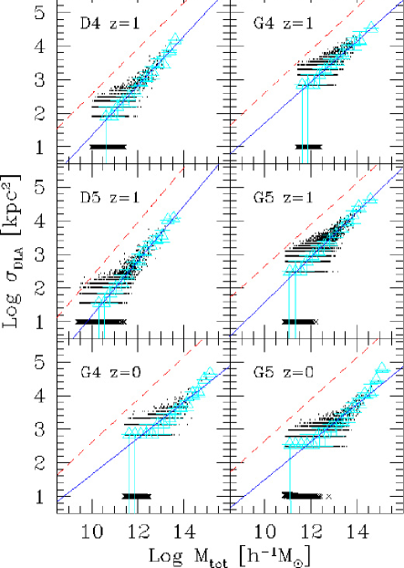
Figure 4: Same as Figure 3, but for $z=1$ and $0$. The short-dashed lines are the fits we obtained at $z=3$, for comparison.

Lower Redshifts

Run	slope $\alpha$	$\beta$
z=1
D4	0.74	2.82
D5	0.82	2.75
G4	0.61	2.93
G5	0.67	2.89
z=0
G4	0.54	2.73
G5	0.56	2.62

Table 4: The parameters obtained by least-square fitting the power-law of equation (7) to the median points shown in Figure 4.

5 Cumulative Abundance of DLAs

Dark matter haloes with masses below the resolution limit of a simulation cannot be resolved. This is a serious problem when one tries to compute the number density of DLAs based on a cosmological simulation that does not resolve all small mass haloes that may host a DLA. Note in particular that the number density of dark matter haloes is known to increase strongly towards lower masses. Even a small incompleteness at low masses will hence prevent a reliable estimate of the DLA abundance if only a simple number count of DLAs found in a cosmological simulation is used.

To overcome this limitation, Gardner et al. (1997a, b, 2001) convolved a theoretical fit to the dark matter halo mass function with the measured relationship between DLA cross-section and halo mass. In this way, they were able to correct for incompleteness in the resolved halo abundance of the simulations. The cumulative abundance (or equivalently the rate of incidence) of DLAs per unit redshift as a function of halo mass in this approach can be expressed as

$$\frac{{\rm d}N_{\rm DLA}}{{\rm d}z}(>M,z)=\frac{{\rm d}r}{{\rm d}z}\int_{M}^{\infty}n_{\rm dm}(M^{\prime},z)~{}\sigma_{\rm DLA}(M^{\prime},z)\,{\rm d}M^{\prime},$$ (8)

where $n_{\rm dm}(M,z)$ is the dark matter halo mass function (for which we use the Sheth & Tormen (1999) parameterisation), and ${\rm d}r/{\rm d}z=c/H(z)$ with $H(z)=H_{0}E(z)=H_{0}\sqrt{\Omega_{\rm m}(1+z)^{3}+\Omega_{\Lambda}}$ for a flat universe. In order to carry out this integral, the power-law fits obtained in Section 4 can be used to represent $\sigma_{\rm DLA}(M,z)$ which give the mean relation between the halo mass and the DLA cross-section. Note that the dependence on the Hubble constant disappears on the right-hand-side of equation (8) because ${\rm d}r/{\rm d}z$ scales as $h^{-1}$, while $n_{\rm dm}{\rm d}M$ depends on $h^{3}$, and $\sigma_{\rm DLA}$ scales as $h^{-2}$ in the simulation.

5.1 DLA abundance at redshift 3

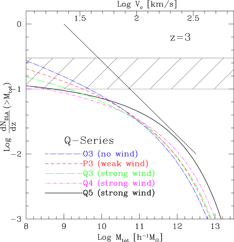
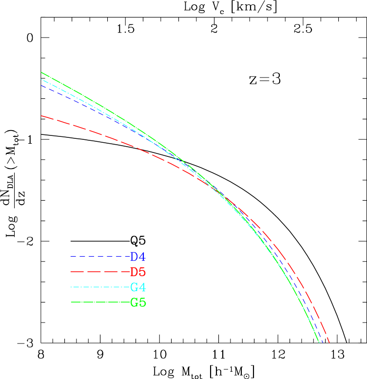
Figure 5: Cumulative abundance (or equivalently rate of incidence) of DLAs per unit redshift as a function of total halo mass. Left panel: Comparison of the results for the Q-series. The runs with a strong wind (Q3, Q4, Q5) have fewer DLAs than those with weak (P3) and no winds (O3). The transition from Q3 to Q4, and then to Q5, shows that higher numerical resolution tends to lead to fewer DLAs. The shaded region indicates the observed DLA abundance of Péroux et al. (2001). The solid slanted line shows the simulation result obtained by Gardner et al. (2001). Right panel: Same as the left panel, but for the D- and the G-series, which all have strong winds. We also include the Q5 run as a thick solid line to ease comparison with the left panel.

In Figure 5, we show the cumulative abundance of DLAs per unit redshift at $z=3$ as a function of total halo mass. The horizontal shaded region in the left panel indicates the observed DLA abundance of Péroux et al. (2001). We note that the data-set analysed by Péroux et al. (2001) includes that of Storrie-Lombardi & Wolfe (2000), and a similar value for the DLA abundance was also reported by Storrie-Lombardi & Wolfe (2000). It is encouraging that the DLA abundances found in our simulations agree well with the observed range.

As we discussed in Section 4.2, the DLA cross-section is falling off rapidly at ${M_{\rm tot}}\sim 10^{8}\,h^{-1}{\rm M_{\odot}}$. Consequently, the DLA abundance per unit redshift can be read off from the cumulative abundance plot at ${M_{\rm tot}}=10^{8}\,h^{-1}{\rm M_{\odot}}$, provided that the underlying simulation can resolve this mass-scale well. For our highest resolution run at $z=3$ (Q5), this is, in fact, the case. Here, the cumulative abundance has already flattened out at ${M_{\rm tot}}=10^{8}\,h^{-1}{\rm M_{\odot}}$, so that a correction with equation (8) for a missed contribution by haloes on smaller mass-scales becomes unnecessary.

In the left panel of Figure 5, it is seen that the DLA abundance decreases as the wind strength increases from O3 to P3, and to Q3, and as the resolution of the simulation increases from Q3 to Q4, and to Q5. This is due to the increasing slope of the power-law fits that we obtained in Section 4. As the slope of the power-law fit increases, the contribution from massive haloes becomes larger, while that from low-mass haloes becomes smaller. As a result, the cumulative abundance at the high-mass end of Figure 5 is largest for Q5, but when summed over all masses, Q5 exhibits the smallest total DLA abundance.

We also show the result from Gardner et al. (2001) as a solid slanted line in the left panel of Figure 5. They argued that their result would be consistent with the observations if the observed DLAs originate only from haloes with circular velocities larger than $v_{c}\sim 60\,\rm km\,s^{-1}$ (which corresponds to ${M_{\rm tot}}\approx 2\times 10^{10}\,h^{-1}{\rm M_{\odot}}$). However, the good agreement between our improved simulations and the observational determinations suggests that Gardner et al. (2001) probably overpredicted the DLA abundance due to the shallower slope they estimated for the relation between the halo mass and the DLA cross-section (see Section 4.1).

In the right panel of Figure 5, the results for the D- and G-series are shown, with the values for Q5 included as a reference to ease comparison with the left panel. As the box-size increases from the Q- to the D-series, and then to the G-series, the resolution of the simulations severely degrades, causing an overprediction for the abundance, for the reasons discussed above. Therefore, we believe that Q5 represents our most reliable estimate at $z=3$ (leaving aside the question whether the feedback strength of the galactic wind adopted for the Q-runs is appropriate or not).

5.2 Redshift evolution of DLA abundance

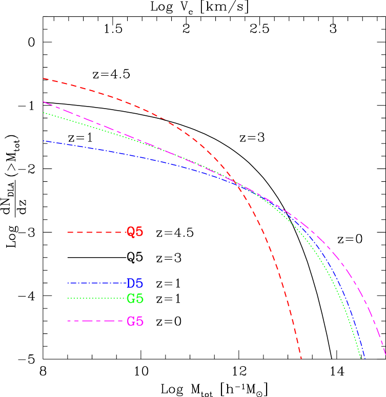
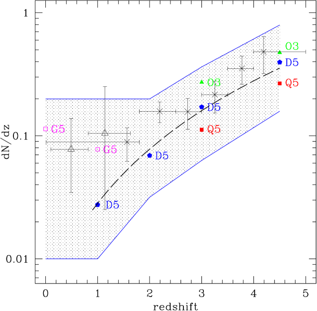
Figure 6: Evolution of the DLA abundance from $z=4.5$ to $z=0$. Left panel: Cumulative DLA abundance as a function of total halo mass at redshifts $z=4.5,3,1$ and 0. Right panel: DLA abundance per unit redshift as a function of redshift. The data points with error bars are the observational data from Péroux et al. (2001) (crosses) and Rao & Turnshek (2000) (open triangles at $z<1.5$). The exact simulation results from some of the runs are indicated by the symbols with run-names. The shaded region is our best-guess for a confidence region based on combining all of our simulations. For reference, we show the power-law of ${\rm d}N/{\rm d}z=N_{0}(1+z)^{\gamma}$ with $N_{0}=0.005$ and $\gamma=2.5$ as a long-dashed line.

In Figure 6, we show the evolution of DLA abundance from $z=4.5$ to $z=0$. In the left panel, the cumulative abundances of DLAs are shown as a function of total halo mass for redshifts $z=4.5,3,1$, and 0. One can see that the contribution from massive haloes to the DLA population progressively increases from high- to low-redshift as a result of the merging of haloes. In the right panel, we give the DLA abundance per unit redshift as a function of epoch, with values here read off at ${M_{\rm tot}}=10^{8}\,h^{-1}{\rm M_{\odot}}$ in the left panel. Observed data points from Péroux et al. (2001) and Rao & Turnshek (2000) are also shown with error bars. Some of the exact simulation results are shown by the symbols, labelled with the names of the corresponding runs. The shaded region is our best-guess for a confidence region based on combining all of our simulation results. For reference, we show a power-law ${\rm d}N/{\rm d}z=N_{0}(1+z)^{\gamma}$ with $N_{0}=0.005$ and $\gamma=2.5$ as a long-dashed line, which describes the rate of evolution seen in the simulations well. It is encouraging that the above value of $\gamma$ is in good agreement with the observed evolution of Lyman-limit systems of Péroux et al. (2001), where they report $\gamma=2.45^{+0.75}_{-0.04}$.

From $z=4.5$ to $z=3$, we see a decrease in the abundance by a factor of about two in both simulations and the observations, and the agreement between the two is very good, although the simulation points tend to fall slightly below the observations. From $z=3$ to $z=1$, the simulation (D5) suggests a further rapid decrease in DLA abundance by a factor of $\sim 6$, which is not seen at this level in the existing observations. But the observational data at low redshift are still relatively uncertain, as indicated by the large error bars. The rapid decline is also reflected in the fact that $\Omega_{\rm HI}$ decreases from 0.66 ($z=3$) to 0.14 ($z=1$) in D5 over this redshift range, a reduction of nearly a factor of 5 (see Figure 1). If this significant decrease in the number of DLAs from $z=3$ to $z=1$ is real, it would partly explain why it is so difficult to find DLAs at $z\leq 1$.

On the other hand, not much evolution is seen from $z=1$ to $z=0$ in the G5 simulation. This is related to the fact that $\Omega_{\rm HI}$ in G5 does not decrease very much from $z=1$ ($\Omega_{\rm HI}=0.19$) to $z=0$ ($\Omega_{\rm HI}=0.16$). However, as discussed earlier, our power-law fits to the $\sigma_{\rm DLA}-{M_{\rm tot}}$ relation are not well constrained for $z=0$ (and possibly for $z=1$ as well), so the results at $z\leq 2$ should be interpreted with caution. At $z\geq 3$, we saw that lower resolution runs tend to predict a larger abundance due to a shallower slope in the relation between the DLA cross-section and the halo mass, but it is not clear if other forms of systematic bias dominate at very low redshift for simulations with poor resolution. We will need yet higher resolution simulations with large box-sizes to make a more robust prediction of the DLA abundance at $z\leq 2$, and until then, it is not clear whether the current results for DLA abundance at $z\leq 2$, which tend to fall below the observational data, are trustworthy. This is why we have widened the shaded confidence region in Figure 6 significantly for $z\leq 2$.

6 Hi  Column Density Distribution Function

The column density distribution function $f(N,X(z))$ is defined such that $f(N,X){\rm d}N{\rm d}X$ is the number of absorbers per sight line with Hi  column densities in the interval $[N,N+{\rm d}N]$, and absorption distances in the interval $[X,X+{\rm d}X]$. The absorption distance $X(z)$ is given by

$$X(z)=\int_{0}^{z}(1+z^{\prime})^{2}\frac{H_{0}}{H(z^{\prime})}{\rm d}z^{\prime}.$$ (9)

This definition is based on an argument by Bahcall & Peebles (1969), who pointed out that the probability of absorption for a quasar sight-line in the redshift interval $[z,z+{\rm d}z]$ is ${\rm d}P\propto(1+z)^{2}{\rm d}r\propto(1+z)^{2}[H_{0}/H(z)]{\rm d}z\equiv{\rm d}X$. In practice, if the comoving box-size of the simulation is $\Delta L$, then the corresponding absorption distance per sight-line is $\Delta X=({H_{0}}/{c})(1+z)^{2}\Delta L$. For example, for $\Delta L=10h^{-1}{\rm\,Mpc}$ and $z=3$, we have $\Delta X=0.0534$.

Assuming that DLAs do not overlap along a sight-line through the simulation volume (which is a very good approximation given the small size of the simulation box, where the expected number of DLAs per sight-line at $z=3$ for a $10h^{-1}{\rm\,Mpc}$ path is $\approx 10^{-3}$), we can compute the ${N_{\rm HI}}$ distribution function by counting the number of grid-cells with column densities in the range $[N,N+{\rm d}N]$. In doing so, we are treating each grid-cell element as one line-of-sight.

6.1 Hi  column density distribution at $z=3$

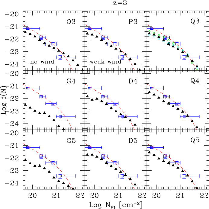
Figure 7: Hi  column density distribution function at $z=3$. The solid triangles are the points measured directly from the simulations. The open squares are the observational data of Péroux et al. (2001, for $2.7<z<3.5$ data), and the dashed line is the fit to the same data based on a gamma-distribution. In the panel for ‘Q3’, the results with different smoothing methods are shown in crosses and open triangles. See text for details.

In Figure 7, we show the Hi  column density distribution function at $z=3$. The solid triangles are the points directly measured from the simulations. The open squares are the observational data of Péroux et al. (2001, for $2.7<z<3.5$ data), and the dashed curve is the fit to the same data based on a gamma-distribution:

$$f(N)=\frac{f_{\ast}}{N_{\ast}}\left(\frac{N}{N_{\ast}}\right)^{-\beta}\exp\left(-\frac{N}{N_{\ast}}\right).$$ (10)

The parameters of the fit are $(f_{\ast},\log N_{\ast},\beta)=(0.0406,21.18,1.10)$ Péroux et al. (2001, for $2.7<z<3.5$ data). We note that all data by Storrie-Lombardi & Wolfe (2000) are included in that of Péroux et al.’s.

In the panel for ‘Q3’ (upper right corner), we also show the result of different smoothing methods, using crosses (uniform cloud-in-cell distribution with $\ell=[{4\pi}/{3}]^{1/3}s$) and open triangles (uniform clouds-in-cell distribution with $\ell=\frac{1}{2}[{4\pi}/{3}]^{1/3}s$). The former method (crosses) results in higher values of $f(N)$ at lower column densities because it smoothes the gas mass into broader regions. The SPH smoothing method agrees with the latter calculation method (open triangles) better.

The agreement between the observations and the simulations Q3, Q4, Q5, & D5 at $\log{N_{\rm HI}}>21$ is generally very good. Results from runs of increasing resolution (Q3, Q4, and Q5) are consistent with each other to a high degree. The run with no wind (O3) somewhat overpredicts the distribution function at large ${N_{\rm HI}}$ values, but as the galactic wind strength increases from O3 to P3, and then to Q3, the high column density systems become less abundant and the agreement between the simulation and observations improves. At intermediate column densities ($20<\log{N_{\rm HI}}<21$), it seems that the simulated distribution function falls short of the observational estimate. Given the consistent behaviour in Q3, Q4, and Q5, our result appears not to be affected by resolution, although this cannot be completely excluded. We will discuss this point further in the next subsection, when we consider the data at $z=4.5$. It is clear however that G4 and G5 do not have sufficient resolution at $z=3$ to resolve DLAs.

6.2 Hi  column density distribution at $z=4.5$

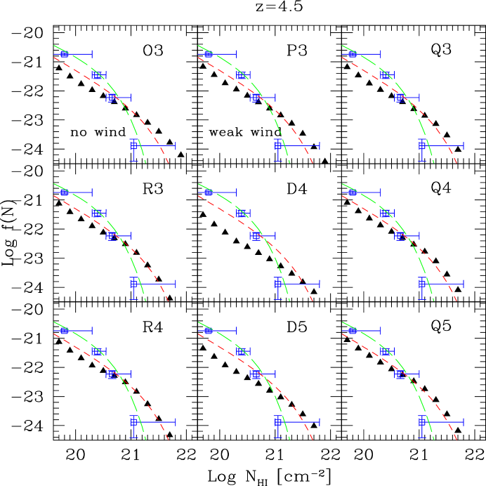
Figure 8: Hi  column density distribution function at $z=4.5$. The solid triangles are the points measured in the simulations, and the open squares are the observational data of Péroux et al. (2001, for $3.5<z<4.99$ data). The long-dashed line is the gamma fit to the same observational data of $3.5<z<4.5$. For comparison, the short-dashed line is the fit to the $2.7<z<3.5$ data.

In Figure 8, we show the Hi  column density distribution function at $z=4.5$. As before, the solid triangles are the points measured in the simulations, and the open squares are the observational data of Péroux et al. (2001, for $3.5<z<4.99$ data). The long-dashed line is the gamma fit to the same observational data of $3.5<z<4.5$, and the short-dashed line is the fit to the data for $2.7<z<3.5$ for reference. The values of the fit parameters for the $3.5<z<4.5$ data is $(f_{\ast},\log N_{\ast},\beta)=(0.2506,20.46,0.80)$.

Observational studies (Storrie-Lombardi & Wolfe, 2000; Péroux et al., 2001) indicate that there are fewer high ${N_{\rm HI}}$ systems ($\log{N_{\rm HI}}>21$) at $z>3.5$ compared with $2.7<z<3.5$, and that the distribution function becomes steeper at $z>3.5$. However, we do not see such a reduction of high ${N_{\rm HI}}$ systems in our simulations from $z=3$ to $z=4$. In fact, the highest resolution simulation in our series (Q5) suggests that $f(N)$ is slightly higher (but steeper at the same time) at $z=4.5$ compared to $z=3$. Note that the agreement between runs with different resolution (Q3, Q4, Q5, R3, and R4) is impressive, showing that the results are well-converged. The degree of the increase in $f(N)$ from $z=3$ to $z=4.5$ is somewhat larger for the intermediate ${N_{\rm HI}}$ systems ($20<\log{N_{\rm HI}}<21$), leading to a slight steepening of the overall $f(N)$. One interpretation is that observational studies have not yet discovered sufficient numbers of DLAs with very high column density ($\log{N_{\rm HI}}>21$) to accurately estimate the evolution of $f(N)$ at $z>3$, because such high ${N_{\rm HI}}$ systems are intrinsically rare and therefore difficult to find.

The evolution from $z=4.5$ to $z=3$ is presumably driven by the combined effect of the depletion of the abundance of small haloes by merging, the accumulation of feedback by galactic winds, and the reduction of cooling efficiency. Small haloes of comparatively low column densities ($\log{N_{\rm HI}}<20.5$) merge into larger systems from $z=4.5$ to $z=3$, forming more massive systems with higher column densities, as the hierarchical structure formation scenario suggests. However, strong feedback by galactic winds ejects neutral gas from the star-forming regions, thereby acting to reduce the column densities of all systems. In addition, the efficiency of cooling rapidly decreases towards lower redshift, reducing the rate at which gas can cool out of haloes and become neutral.

6.3 Hi  column density distribution at lower redshift

In Figure 9, we show the Hi  column density distribution function at $z=1$ and $z=0$. Again, solid triangles give the points measured in the simulations, and the open squares are the observational data of Péroux et al. (2001, for $0.008<z<2.0$ data). The dashed curve is the gamma-distribution fit to the same observational data with parameters $(f_{\ast},\log N_{\ast},\beta)=(0.0870,20.76,0.74)$. For comparison, we also show the observational gamma fit for $2.7<z<3.5$ data as dotted lines.

As we pointed out earlier, the results of the G-series are substantially affected by resolution, causing an underestimate of the DLA abundance if it is not corrected using equation (8). (If the abundance is corrected with an ill-determined relation between the DLA cross-section and the halo mass, then low resolution can also lead to an overestimate of the abundance, as we discussed in Section 5.) With the mass resolution of the G-series, haloes with ${M_{\rm tot}}<10^{10}\,h^{-1}{\rm M_{\odot}}$ are not resolved, and a significant fraction of the DLA population is therefore missed. Curiously, it is seen that the column density distribution function in fact rises from $z=1$ to $z=0$ in the G-series. This is probably because haloes with masses above the mass resolution limit are only beginning to form at these low redshifts as the non-linear mass-scale increases with decreasing redshift, and the simulation is finally “catching up” to reproduce the neutral gas content in these haloes.

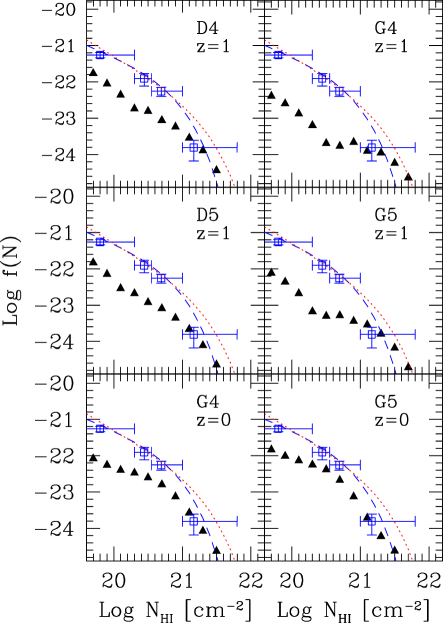
Figure 9: Hi  column density distribution function at $z=1$ and $z=0$. The solid triangles are the points measured in the simulations, and the open squares are the observational data of Péroux et al. (2001, for $0.008<z<2.0$ data). The dashed curve is the gamma-distribution fit to the same observational data. For comparison, we also show the observational gamma fit for $2.7<z<3.5$ data as dotted lines.

7 Discussion

We have used state-of-the-art hydrodynamic simulations of structure formation to investigate the abundance of DLAs in a $\Lambda$CDM universe. Our study represents a first attempt to apply a large series of simulations to this problem, probing an unprecedented range in both mass and spatial scales, enabling us to quantify systematic effects due to numerical resolution. Furthermore, we improved the simulation methodology by adopting a novel formulation of SPH (see Springel & Hernquist, 2002) that minimises systematic inaccuracies in simulations with cooling, and by using an improved model for the treatment of the multiphase structure of the ISM in the context of star formation and feedback (Springel & Hernquist, 2003a).

By comparing our results for DLA abundance in a series of runs as a function of resolution and feedback strength, we were able to demonstrate that insufficient resolution, or a lack of a proper treatment of effective feedback processes, leads to an incorrect estimate of the relation between the DLA cross-section and the halo mass. This likely led to an overestimate of the DLA abundance in earlier studies, for the reasons we discussed in detail in Section 4.1.

Prochaska & Wolfe (2001) pointed out that the observed velocity width distribution cannot be reproduced if the relation between the DLA cross-section and the halo mass derived from these earlier SPH simulations is used. They also suggested that one possibility to remedy this inconsistency was to suppose that the relationship between the DLA cross-section and the halo mass was incorrectly determined. This is exactly what we find in our current study. If we use the new relation found in our highest resolution simulation, we obtain a DLA abundance that is consistent with observations, which is very encouraging. The slope of the relation that we infer from our simulations at $z=3$ is in the range of $0.7-1.0$, which coincides with the range that Haehnelt, Steinmetz, & Rauch (2000) derived by requiring their model prediction of velocity width distribution to match the observed one.

However, while our simulations reproduce the DLA abundance at $z=3$ very well, our predictions at $z\leq 2$ are not equally reliable because they are based on simulations with larger box-sizes and lower resolution. This is also evident from the poor agreement between the simulated and the observed Hi  column density distribution function at low redshift. To make the predictions at low-redshift more robust will require large box-size simulations with yet more particles.

The fact that we were able to reproduce the observed DLA abundance very well at redshift $z=3$ has significant implications for the cold dark matter model. This result suggests that DLAs arise naturally in a $\Lambda$CDM universe from radiatively cooled gas in dark matter haloes with correct abundance. This is related to the “substructure problem” that is posed against the CDM model, based on the notion that the number of satellite galaxies observed around the Milky Way seems to be much smaller than, and hence in contradiction to, the large number of dark matter substructures predicted by high-resolution N-body simulations (Moore et al., 1999).

Stoehr, White, Tormen & Springel (2002) have shown that the seriousness of this discrepancy was overstated initially, but the high abundance of low mass haloes and dark satellites in CDM models remains puzzling, given for example the shallow faint-end slope of the galaxy luminosity function. Therefore, many models have been invoked to suppress the formation of dwarf satellite galaxies, including supernova feedback that ejects gas (Dekel & Silk, 1986), reheating of the intergalactic medium which suppresses gas infall (Bullock, Kravtsov, & Weinberg, 2001), and photoionisation of gas by UV background radiation (Thoul & Weinberg, 1996; Quinn, Katz, & Efstathiou, 1996). Full cosmological hydro-simulations have also been used to argue that feedback effects by UV background radiation and supernovae may account for the suppression of the formation of low-mass galaxies relative to the steeply rising dark matter halo mass function (Chiu, Ostriker, & Gnedin, 2001; Nagamine et al., 2001b). While we cannot make a strong statement on this problem at low-redshift, our results suggest that the CDM model does not have difficulty at $z=3$ with respect to the number of neutral gas clumps from which stars form. Considering that there is in general good agreement between observations and theoretical studies of Lyman-break galaxies at $z=3$ (e.g. Mo & Fukugita, 1996; Baugh et al., 1998; Jing & Suto, 1998; Katz, Hernquist & Weinberg, 1999; Kauffmann et al., 1999; Mo, Mao, & White, 1999; Nagamine, 2002; Weinberg, Hernquist & Katz, 2002), the $\Lambda$CDM model seems to be in a very good shape at $z=3$.

Another interesting result of our study is that the break in the relation between DLA cross-section and halo mass seems to occur at a mass-scale of ${M_{\rm tot}}\approx 10^{8}-10^{8.5}\,h^{-1}{\rm M_{\odot}}$. DLAs do not exist in haloes below this mass-scale at $z=3$ and $z=4.5$. Because we measured this effect consistently in both the ‘Q5’ and ‘R4’-runs, which have sufficient resolution to describe haloes with ${M_{\rm tot}}=10^{8}\,h^{-1}{\rm M_{\odot}}$ well, it is clear that this is not caused by a resolution effect. Note that this mass-scale, which corresponds to circular velocities of $10-15\,\rm km\,s^{-1}$ and virial temperatures of about $10^{4}\,{\rm K}$ or even slightly lower, is smaller than suggested by the earlier studies of Quinn, Katz, & Efstathiou (1996) and Thoul & Weinberg (1996) (See also Weinberg, Hernquist & Katz (1997)). The physical origin of the break could lie in both the radiative processes of cooling and UV-heating, and in supernovae feedback, but we expect that the former effects dominate. This is because feedback will proceed only if at least some neutral gas is built up, so that star formation can occur at some (low) level. Only after that can feedback quench the further accumulation of neutral gas, and possibly also affect neighbouring haloes. Therefore, while one can easily understand why supernovae feedback reduces the amount of neutral gas in small halos, it is not clear how it could lead to the complete absence of neutral gas below a certain mass-scale. On the other hand, a relatively sharp break can be expected from the properties of the cooling function, and the heating of the gas due to the UV background. Both processes depend very sensitively on the virial temperature of halos in the range $10^{4}-10^{5}$ K. Further studies will be needed to disentangle the relative importance of the various physical effects in this regime more precisely.

Assuming that feedback effects due to star formation nevertheless influence the mass-scale of the break, we might have underestimated it if the feedback we employed in our simulations was not strong enough. However, we saw in our results of Figure 1 that the current simulations with the ‘strong wind’ model already seem to underpredict $\Omega_{\rm HI}$ slightly, therefore even stronger feedback would make the neutral gas fraction in the Q-series even smaller and exacerbate the discrepancy with the observational estimate of $\Omega_{\rm HI}$ at $z=3$. Also, there is only very limited room to increase the strength of the UV background flux, because for our chosen normalisation the mean opacity of the Lyman-$\alpha$ forest is in good agreement with observations. Another way of constraining the feedback strength is to compare the simulated galaxy luminosity function with the observed one, to see if the flatness of the faint-end of the luminosity function can be reproduced. A preliminary analysis suggests that our present simulations do not yet yield a luminosity function with a faint-end as flat as observed at low-redshift; therefore the feedback model in our current simulation might not be adequate to correctly account for the galaxy population at $z=0$. The results of this analysis will be presented elsewhere. A solution to this problem will help to further constrain the physical processes that suppress the DLA cross-section in low-mass haloes.

In the present paper, we focused on the abundance of DLAs, without carrying out a detailed study of their internal structure. Therefore, we are not able to completely rule out the possibility that the DLAs we find in our simulations are in fact originating from very small disks at the center of dark matter haloes. Our present work is complementary to that of Haehnelt et al. (1998), in the sense that we are able to sample a large statistical ensemble of absorbers in comoving volume of $\geq(10h^{-1}{\rm\,Mpc})^{3}$, while they studied a smaller number of objects in greater detail. Nevertheless, our highest resolution run (Q5) with $10h^{-1}{\rm\,Mpc}$ box has a spatial resolution of $1.2h^{-1}{\rm\,kpc}$ which is comparable to that of Haehnelt et al. (1998), and the results from varying resolution runs (Q3, Q4, Q5) agree with each other well. Therefore, given that our simulations are based on the CDM model, our results support the idea that DLAs arise from radiatively cooled protogalactic gas clumps embedded in dark matter haloes. While our spatial resolution is approaching comoving sub-kpc scales at $z=3$, it is probably not yet sufficient to accurately resolve the disk structures embedded in the central few kpc regions of dark matter haloes. Kinematical studies of the internal structure of DLAs will require yet higher resolution simulations than those used in the present paper, and possibly a more sophisticated physical model for the ISM and star formation.

References

- Adelberger et al. (2002) Adelberger K. L., Steidel C. C., Shapley A. E., Pettini M., 2002, ApJ, 584, 45
- Adelberger et al. (1998) Adelberger K. L., Steidel C. C., Giavalisco M., Dickinson M., Pettini M., Kellogg M., 1998, ApJ, 505, 18
- Aguirre et al. (2001a) Aguirre A., Hernquist L., Schaye J., Weinberg D., Katz N., Gardner J., 2001a, ApJ, 560, 599
- Aguirre et al. (2001b) Aguirre A., Hernquist L., Schaye J., Katz N., Weinberg D., Gardner J., 2001b, ApJ, 561, 521
- Bahcall & Peebles (1969) Bahcall J. N., Peebles P. J. E., 1969, ApJ, 156, L7
- Baugh et al. (1998) Baugh C. M., Cole S., Frenk C. S., Lacey C. G., 1998, ApJ, 498, 504
- Becker et al. (2001) Becker R. H., et al., 2001, AJ, 122, 2850
- Blain et al. (1999) Blain A. W., Smail I., Ivison R. J., Kneib J.-P., 1999, MNRAS, 302, 632
- Bullock, Kravtsov, & Weinberg (2001) Bullock J. S., Kravtsov A. V., Weinberg D. H., 2000, ApJ, 539, 517
- Chiu, Ostriker, & Gnedin (2001) Chiu W. A., Gnedin N. Y., Ostriker J. P., 2001, ApJ, 563, 21
- Croft et al. (2001) Croft R. A. C., Di Matteo T., Davé R., Hernquist L., Katz N., Fardal M. A., Weinberg D.H., 2001, ApJ, 557, 67
- Croft et al. (2002) Croft R. A. C., Hernquist L., Springel V., Westover M., White M., 2002, ApJ, 580, 634
- Davé et al. (1999) Davé R., Hernquist L., Katz N., Weinberg D. H., 1999, ApJ, 511, 521
- Dekel & Silk (1986) Dekel A, Silk J., 1986, ApJ, 303, 39
- Gardner et al. (1997a) Gardner J. P., Katz N., Hernquist L., Weinberg D. H., 1997a, ApJ, 484, 31
- Gardner et al. (1997b) Gardner J. P., Katz N., Weinberg D. H., Hernquist L., 1997b, ApJ, 486, 42
- Gardner et al. (2001) Gardner J. P., Katz N., Hernquist L., Weinberg D. H., 2001, ApJ, 559, 131
- Haardt & Madau (1996) Haardt F., Madau P., 1996, ApJ, 461, 20
- Haehnelt, Steinmetz, & Rauch (2000) Haehnelt M., Steinmetz M., Rauch M., 2000, ApJ, 534, 594
- Haehnelt, Steinmetz, & Rauch (1998) Haehnelt M., Steinmetz M., Rauch M., 1998, ApJ, 495, 647
- Hernquist (1993) Hernquist L., 1993, ApJ, 404, 717
- Hernquist & Springel (2002) Hernquist L., Springel V., 2003, MNRAS, 341, 1253
- Hernquist et al. (1996) Hernquist L., Katz N., Weinberg D. H., Miralda-Escudé J., 1996, ApJ, 457, L51
- Jing & Suto (1998) Jing Y. P., Suto Y., 1998, ApJ, 494, L5
- Katz, Hernquist & Weinberg (1999) Katz N., Hernquist L., Weinberg D. H., 1999, ApJ, 523, 463
- Katz et al. (1996) Katz N., Weinberg D. H., Hernquist L., 1996, ApJS, 105, 19
- Katz et al. (1996) Katz N., Weinberg D. H., Hernquist L., Miralda-Escudé J., 1996, ApJ, 457, L57
- Kauffmann et al. (1999) Kauffmann G. A. M., Colberg J. M., Diaferio A., White S. D. M., 1999, MNRAS, 307, 529
- Kollmeier et al. (2003) Kollmeier J. A., Weinberg D. H., Davé R., Katz N., 2003, ApJ, submitted (astro-ph/0209563)
- Kulkarni et al. (2001) Kulkarni V. P., Hill J. M., Schneider G., Weymann R. J., Storrie-Lombardi L. J., Rieke M. J., Thompson R. I., Jannuzi B. T., 2001, ApJ, 551, 37
- Kulkarni et al. (2000) Kulkarni V. P., Hill J. M., Schneider G., Weymann R. J., Storrie-Lombardi L. J., Rieke M. J., Thompson R. I., Jannuzi B. T., 2000, ApJ, 536, 36
- Lanzetta et al. (2002) Lanzetta K. M., Yahata N., Pascarelle S., Chen H-W., Fernández-Soto A., 2002, ApJ, 570, 492
- Le Brun et al. (1997) Le Brun V., Bergeron J., Boissé P., Deharveng J. M., 1997, A&A, 321, 733
- Lucy (1977) Lucy L., 1977, AJ, 82, 1013
- Mo & Fukugita (1996) Mo H. J., Fukugita, 1996, ApJ, 467, L9
- Mo, Mao, & White (1999) Mo H. J., Mao S., White S. D. M., 1999, MNRAS, 304, 175
- Moore et al. (1999) Moore B., Ghigna S., Governato F., Lake G., Quinn T., Stadel, J., Tozzi P., 1999, ApJ, 524, L19
- Nagamine (2002) Nagamine K., 2002, ApJ, 564, 73
- Nagamine et al. (2001a) Nagamine K., Fukugita M., Cen R., Ostriker J. P., 2001a, ApJ, 558, 497
- Nagamine et al. (2001b) Nagamine K., Fukugita M., Cen R., Ostriker J. P., 2001b, MNRAS, 327, L10
- Pascarelle, Lanzetta, & Fernández-Soto (1998) Pascarelle S., Lanzetta K. M., Fernández-Soto A., 1998, ApJ, 508, L1
- Pearce et al. (1999) Pearce et al., 1999, ApJ, 521, 99
- Péroux et al. (2001) Péroux C., McMahon R. G., Storrie-Lombardi L. J., Irwin M. J., in ”Chemical Enrichment of Intracluster and Intergalactic medium”, Proceedings of the Vulcano Workshop, May 14-18, 2001 (astro-ph/0107045)
- Pettini et al. (2002) Pettini M., Rix S. A., Steidel C. C., Adelberger K. L., Hunt M. P., Shapley A. E. 2002, ApJ, 569, 742
- Press & Schechter (1974) Press W. H., Schechter P., 1974, ApJ, 187, 425
- Prochaska & Wolfe (2001) Prochaska J. X. & Wolfe A. M., 2001, ApJ, 560, L33
- Prochaska & Wolfe (1998) Prochaska J. X. & Wolfe A. M., 1998, ApJ, 507, 113
- Prochaska & Wolfe (1997) Prochaska J. X. & Wolfe A. M., 1997, ApJ, 487, 73
- Quinn, Katz, & Efstathiou (1996) Quinn T., Katz N., Efstathiou G., 1996, MNRAS, 278, L49
- Rao & Turnshek (1998) Rao S. M., Turnshek D. A., 1998, ApJ, 500, L115
- Rao & Turnshek (2000) Rao S. M., Turnshek D. A., 2000, ApJS, 130, 1
- Shapley et al. (2001) Shapley A. E., Steidel C. C., Adelberger K. L., Dickinson M., Giavalisco M., Pettini M. 2001, ApJ, 562, 95
- Sheth & Tormen (1999) Sheth R. V., Tormen G., 1999, MNRAS, 308, 119
- Sokasian et al. (2003) Sokasian A., Hernquist L., Abel T. Springel V., 2003, MNRAS, in press (astro-ph/0303098)
- Springel, Yoshida & White (2001) Springel V., Yoshida N., White S. D. M., 2001, New Astronomy, 6, 79
- Springel & Hernquist (2002) Springel V., Hernquist L., 2002, MNRAS, 333, 649
- Springel & Hernquist (2003a) Springel V., Hernquist L., 2003a, MNRAS, 339, 289
- Springel & Hernquist (2003b) Springel V., Hernquist L., 2003b, MNRAS, 339, 312
- Steidel et al. (1999) Steidel C. C., Adelberger K. L., Giavalisco M., Dickinson M., Pettini, M., 1999, ApJ, 519, 1