General solution of the Jeans equations for triaxial galaxies with separable potentials

Abstract

The Jeans equations relate the second-order velocity moments to the density and potential of a stellar system. For general three-dimensional stellar systems, there are three equations and six independent moments. By assuming that the potential is triaxial and of separable Stäckel form, the mixed moments vanish in confocal ellipsoidal coordinates. Consequently, the three Jeans equations and three remaining non-vanishing moments form a closed system of three highly-symmetric coupled first-order partial differential equations in three variables. These equations were first derived by Lynden–Bell, over 40 years ago, but have resisted solution by standard methods. We present the general solution here.

We consider the two-dimensional limiting cases first. We solve their Jeans equations by a new method which superposes singular solutions. The singular solutions, which are new, are standard Riemann–Green functions. The resulting solutions of the Jeans equations give the second moments throughout the system in terms of prescribed boundary values of certain second moments. The two-dimensional solutions are applied to non-axisymmetric discs, oblate and prolate spheroids, and also to the scale-free triaxial limit. There are restrictions on the boundary conditions which we discuss in detail. We then extend the method of singular solutions to the triaxial case, and obtain a full solution, again in terms of prescribed boundary values of second moments. There are restrictions on these boundary values as well, but the boundary conditions can all be specified in a single plane. The general solution can be expressed in terms of complete (hyper)elliptic integrals which can be evaluated in a straightforward way, and provides the full set of second moments which can support a triaxial density distribution in a separable triaxial potential.

1 Introduction

Much has been learned about the mass distribution and internal dynamics of galaxies by modeling their observed kinematics with solutions of the Jeans equations (e.g., Binney & Tremaine 1987). These are obtained by taking velocity moments of the collisionless Boltzmann equation for the phase-space distribution function $f$, and connect the second moments (or the velocity dispersions, if the mean streaming motion is known) directly to the density and the gravitational potential of the galaxy, without the need to know $f$. In nearly all cases there are fewer Jeans equations than velocity moments, so that additional assumptions have to be made about the degree of anisotropy. Furthermore, the resulting second moments may not correspond to a physical distribution function $f\geq 0$. These significant drawbacks have not prevented wide application of the Jeans approach to the kinematics of galaxies, even though the results need to be interpreted with care. Fortunately, efficient analytic and numerical methods have been developed in the past decade to calculate the full range of distribution functions $f$ that correspond to spherical or axisymmetric galaxies, and to fit them directly to kinematic measurements (e.g., Gerhard 1993; Qian et al. 1995; Rix et al. 1997; van der Marel et al. 1998). This has provided, for example, accurate intrinsic shapes, mass-to-light ratios, and central black hole masses (e.g., Verolme et al. 2002; Gebhardt et al. 2003).

Many galaxy components are not spherical or axisymmetric, but have triaxial shapes (Binney 1976, 1978). These include early-type bulges, bars, and giant elliptical galaxies. In this geometry, there are three Jeans equations, but little use has been made of them, as they contain six independent second moments, three of which have to be chosen ad-hoc (see, e.g., Evans, Carollo & de Zeeuw 2000). At the same time, not much is known about the range of physical solutions, as very few distribution functions have been computed, and even fewer have been compared with kinematic data (but see Zhao 1996).

An exception is provided by the special set of triaxial mass models that have a gravitational potential of Stäckel form. In these systems, the Hamilton–Jacobi equation separates in orthogonal curvilinear coordinates (Stäckel 1891), so that all orbits have three exact integrals of motion, which are quadratic in the velocities. The associated mass distributions can have arbitrary central axis ratios and a large range of density profiles, but they all have cores rather than central density cusps, which implies that they do not provide perfect fits to galaxies (de Zeeuw, Peletier & Franx 1986). Even so, they capture much of the rich internal dynamics of large elliptical galaxies (de Zeeuw 1985a, hereafter Z85; Statler 1987, 1991; Arnold, de Zeeuw & Hunter 1994). Numerical and analytic distribution functions have been constructed for these models (e.g., Bishop 1986; Statler 1987; Dejonghe & de Zeeuw 1988; Hunter & de Zeeuw 1992, hereafter HZ92; Mathieu & Dejonghe 1999), and their projected properties have been used to provide constraints on the intrinsic shapes of individual galaxies (e.g., Statler 1994a, b; Statler & Fry 1994; Statler, DeJonghe & Smecker-Hane 1999; Bak & Statler 2000; Statler 2001).

The Jeans equations for triaxial Stäckel systems have received little attention. This is remarkable, as Eddington (1915) already knew that the velocity ellipsoid in these models is everywhere aligned with the confocal ellipsoidal coordinate system in which the motion separates. This means that there are only three, and not six, non-vanishing second-order velocity moments in these coordinates, so that the Jeans equations form a closed system. However, Eddington, and later Chandrasekhar (1939, 1940), did not study the velocity moments, but instead assumed a form for the distribution function, and then determined which potentials are consistent with it. Lynden–Bell (1960) was the first to derive the explicit form of the Jeans equations for the triaxial Stäckel models. He showed that they constitute a highly symmetric set of three first-order partial differential equations (PDEs) for three unknowns, each of which is a function of the three confocal ellipsoidal coordinates, but he did not derive solutions. When it was realized that the orbital structure in the triaxial Stäckel models is very similar to that in the early numerical models for triaxial galaxies with cores (Schwarzschild 1979; Z85), interest in the second moments increased, and the Jeans equations were solved for a number of special cases. These include the axisymmetric limits and elliptic discs (Dejonghe & de Zeeuw 1988; Evans & Lynden–Bell 1989, hereafter EL89), triaxial galaxies with only thin tube orbits (HZ92), and, most recently, the scale-free limit (Evans et al. 2000). In all these cases the equations simplify to a two-dimensional problem, which can be solved with standard techniques after recasting two first-order equations into a single second-order equation in one dependent variable. However, these techniques do not carry over to a single third-order equation in one dependent variable, which is the best that one could expect to have in the general case. As a result, the general case has remained unsolved.

In this paper, we first present an alternative solution method for the two-dimensional limiting cases which does not use the standard approach, but instead uses superpositions of singular solutions. We show that this approach can be extended to three dimensions, and provides the general solution for the triaxial case in closed form, which we give explicitly. We will apply our solutions in a follow-up paper, and will use them together with the mean streaming motions (Statler 1994a) to study the properties of the observed velocity and dispersion fields of triaxial galaxies.

In §2, we define our notation and derive the Jeans equations for the triaxial Stäckel models in confocal ellipsoidal coordinates, together with the continuity conditions. We summarise the limiting cases, and show that the Jeans equations for all the cases with two degrees of freedom correspond to the same two-dimensional problem. We solve this problem in §3, first by employing a standard approach with a Riemann–Green function, and then via the singular solution superposition method. We also discuss the choice of boundary conditions in detail. We relate our solution to that derived by EL89 in Appendix A, and explain why it is different. In §4, we extend the singular solution approach to the three-dimensional problem, and derive the general solution of the Jeans equations for the triaxial case. It contains complete (hyper)elliptic integrals, which we express as single quadratures that can be numerically evaluated in a straightforward way. We summarise our conclusions in §5.

2 The Jeans equations for separable models

We first summarise the essential properties of the triaxial Stäckel models in confocal ellipsoidal coordinates. Further details can be found in Z85. We show that for these models the mixed second-order velocity moments vanish, so that the Jeans equations form a closed system. We derive the Jeans equations and find the corresponding continuity conditions for the general case of a triaxial galaxy. We then give an overview of the limiting cases and show that solving the Jeans equations for the various cases with two degrees of freedom reduces to an equivalent two-dimensional problem.

2.1 Triaxial Stäckel models

We define confocal ellipsoidal coordinates ($\lambda,\mu,\nu$) as the three roots for $\tau$ of

$$\frac{x^{2}}{\tau+\alpha}+\frac{y^{2}}{\tau+\beta}+\frac{z^{2}}{\tau+\gamma}=1,$$ (2.1)

with ($x,y,z$) the usual Cartesian coordinates, and with constants $\alpha,\beta$ and $\gamma$ such that $-\gamma\leq\nu\leq-\beta\leq\mu\leq-\alpha\leq\lambda$. For each point ($x,y,z$), there is a unique set ($\lambda,\mu,\nu$), but a given combination ($\lambda,\mu,\nu$) generally corresponds to eight different points ($\pm x,\pm y,\pm z$). We assume all three-dimensional Stäckel models in this paper to be likewise eightfold symmetric.

Surfaces of constant $\lambda$ are ellipsoids, and surfaces of constant $\mu$ and $\nu$ are hyperboloids of one and two sheets, respectively (Fig. 1). The confocal ellipsoidal coordinates are approximately Cartesian near the origin and become a conical coordinate system at large radii with a system of spheres together with elliptic and hyperbolic cones (Fig. 3). At each point, the three coordinate surfaces are perpendicular to each other. Therefore, the line element is of the form $ds^{2}=P^{2}d\lambda^{2}+Q^{2}d\mu^{2}+R^{2}d\nu^{2}$, with the metric coefficients

$$P^{2} = \frac{(\lambda-\mu)(\lambda-\nu)}{4(\lambda+\alpha)(\lambda+\beta)(\lambda+\gamma)},$$

$$Q^{2} = \frac{(\mu-\nu)(\mu-\lambda)}{4(\mu+\alpha)(\mu+\beta)(\mu+\gamma)},$$ (2.2)

$$R^{2} = \frac{(\nu-\lambda)(\nu-\mu)}{4(\nu+\alpha)(\nu+\beta)(\nu+\gamma)}.$$

We restrict attention to models with a gravitational potential $V_{S}(\lambda,\mu,\nu)$ of Stäckel form (Weinacht 1924)

$$V_{S}=-\frac{F(\lambda)}{(\lambda\!-\!\mu)(\lambda\!-\!\nu)}-\frac{F(\mu)}{(\mu\!-\!\nu)(\mu\!-\!\lambda)}-\frac{F(\nu)}{(\nu\!-\!\lambda)(\nu\!-\!\mu)},$$ (2.3)

where $F(\tau)$ is an arbitrary smooth function.

Adding any linear function of $\tau$ to $F(\tau)$ changes $V_{S}$ by at most a constant, and hence has no effect on the dynamics. Following Z85, we use this freedom to write

$$F(\tau)=(\tau+\alpha)(\tau+\gamma)G(\tau),$$ (2.4)

where $G(\tau)$ is smooth. It equals the potential along the intermediate axis. This choice will simplify the analysis of the large radii behaviour of the various limiting cases.

The density $\rho_{S}$ that corresponds to $V_{S}$ can be found from Poisson’s equation or by application of Kuzmin’s (1973) formula (see de Zeeuw 1985b). This formula shows that, once we have chosen the central axis ratios and the density along the short axis, the mass model is fixed everywhere by the requirement of separability. For centrally concentrated mass models, $V_{S}$ has the $x$-axis as long axis and the $z$-axis as short axis. In most cases this is also true for the associated density (de Zeeuw et al. 1986).

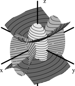
Figure 1: Confocal ellipsoidal coordinates. Surfaces of constant $\lambda$ are ellipsoids, surfaces of constant $\mu$ are hyperboloids of one sheet and surfaces of constant $\nu$ are hyperboloids of two sheets.

2.2 Velocity moments

A stellar system is completely described by its distribution function (DF), which in general is a time-dependent function $f$ of the six phase-space coordinates ($\mathbf{x},\mathbf{v}$). Assuming the system to be in equilibrium ($df/dt=0$) and in steady-state ($\partial f/\partial t=0$), the DF is independent of time $t$ and satisfies the (stationary) collisionless Boltzmann equation (CBE). Integration of the DF over all velocities yields the zeroth-order velocity moment, which is the density $\rho$ of the stellar system. The first- and second-order velocity moments are defined as

$$\langle v_{i}\rangle(\mathbf{x})\!\!\! = \!\!\!\frac{1}{\rho}\iiint v_{i}f(\mathbf{x},\mathbf{v})\;{\mathrm{d}}^{3}v,$$

$$\langle v_{i}v_{j}\rangle(\mathbf{x})\!\!\! = \!\!\!\frac{1}{\rho}\iiint v_{i}v_{j}f(\mathbf{x},\mathbf{v})\;{\mathrm{d}}^{3}v,$$

where $i,j=1,2,3$. The streaming motions $\langle v_{i}\rangle$ together with the symmetric second-order velocity moments $\langle v_{i}v_{j}\rangle$ provide the velocity dispersions $\sigma_{ij}^{2}=\langle v_{i}v_{j}\rangle-\langle v_{i}\rangle\langle v_{j}\rangle$.

The continuity equation that results from integrating the CBE over all velocities, relates the streaming motion to the density $\rho$ of the system. Integrating the CBE over all velocities after multiplication by each of the three velocity components, provides the Jeans equations, which relate the second-order velocity moments to $\rho$ and $V$, the potential of the system. Therefore, if the density and potential are known, we in general have one continuity equation with three unknown first-order velocity moments and three Jeans equations with six unknown second-order velocity moments.

The potential (2.3) is the most general form for which the Hamilton–Jacobi equation separates (Stäckel 1890; Lynden–Bell 1962b; Goldstein 1980). All orbits have three exact isolating integrals of motion, which are quadratic in the velocities (e.g., Z85). It follows that there are no irregular orbits, so that Jeans’ (1915) theorem is strictly valid (Lynden–Bell 1962a; Binney 1982) and the DF is a function of the three integrals. The orbital motion is a combination of three independent one-dimensional motions — either an oscillation or a rotation — in each of the three ellipsoidal coordinates. Different combinations of rotations and oscillations result in four families of orbits in triaxial Stäckel models (Kuzmin 1973; Z85): inner (I) and outer (O) long-axis tubes, short (S) axis tubes and box orbits. Stars on box orbits carry out an oscillation in all three coordinates, so that they provide no net contribution to the mean streaming. Stars on I- and O-tubes carry out a rotation in $\nu$ and those on S-tubes a rotation in $\mu$, and oscillations in the other two coordinates. The fractions of clockwise and counterclockwise stars on these orbits may be unequal. This means that each of the tube families can have at most one nonzero first-order velocity moment, related to $\rho$ by the continuity equation. Statler (1994a) used this property to construct velocity fields for triaxial Stäckel models. It is not difficult to show by similar arguments (e.g., HZ92) that all mixed second-order velocity moments also vanish

$$\langle v_{\lambda}v_{\mu}\rangle=\langle v_{\mu}v_{\nu}\rangle=\langle v_{\nu}v_{\lambda}\rangle=0.$$ (2.6)

Eddington (1915) already knew that in a potential of the form (2.3), the axes of the velocity ellipsoid at any given point are perpendicular to the coordinate surfaces, so that the mixed second-order velocity moments are zero. We are left with three second-order velocity moments, $\langle v_{\lambda}^{2}\rangle$, $\langle v_{\mu}^{2}\rangle$ and $\langle v_{\nu}^{2}\rangle$, related by three Jeans equations.

2.3 The Jeans equations

The Jeans equations for triaxial Stäckel models in confocal ellipsoidal coordinates were first derived by Lynden–Bell (1960). We give an alternative derivation here, using the Hamilton equations.

We first write the DF as a function of ($\lambda,\mu,\nu$) and the conjugate momenta

$$p_{\lambda}=P^{2}\frac{d\lambda}{dt},\quad p_{\mu}=Q^{2}\frac{d\mu}{dt},\quad p_{\nu}=R^{2}\frac{d\nu}{dt},$$ (2.7)

with the metric coefficients $P$, $Q$ and $R$ given in (2.1). In these phase-space coordinates the steady-state CBE reads

$$\frac{d\tau}{dt}\frac{\partial f}{\partial\tau}+\frac{dp_{\tau}}{dt}\frac{\partial f}{\partial p_{\tau}}=0,$$ (2.8)

where we have used the summation convention with respect to $\tau=\lambda,\mu,\nu$. The Hamilton equations are

$$\frac{d\tau}{dt}=\frac{\partial H}{\partial p_{\tau}},\quad\frac{dp_{\tau}}{dt}=\frac{\partial H}{\partial\tau},$$ (2.9)

with the Hamiltonian defined as

$$H=\frac{p_{\lambda}^{2}}{2P^{2}}+\frac{p_{\mu}^{2}}{2Q^{2}}+\frac{p_{\nu}^{2}}{2R^{2}}+V(\lambda,\mu,\nu).$$ (2.10)

The first Hamilton equation in (2.9) defines the momenta (2.7) and gives no new information. The second gives

$$\frac{dp_{\lambda}}{dt}=\frac{p_{\lambda}^{2}}{P^{3}}\frac{\partial P}{\partial\lambda}+\frac{p_{\mu}^{2}}{Q^{3}}\frac{\partial Q}{\partial\lambda}+\frac{p_{\nu}^{2}}{R^{3}}\frac{\partial R}{\partial\lambda}-\frac{\partial V}{\partial\lambda},$$ (2.11)

and similar for $p_{\mu}$ and $p_{\nu}$ by replacing the derivatives with respect to $\lambda$ by derivatives to $\mu$ and $\nu$, respectively.

We assume the potential to be of the form $V_{S}$ defined in (2.3), and we substitute (2.7) and (2.11) in the CBE (2.8). We multiply this equation by $p_{\lambda}$ and integrate over all momenta. The mixed second moments vanish (2.6), so that we are left with

$$\frac{3\langle fp_{\lambda}^{2}\rangle}{P^{3}}\frac{\partial P}{\partial\lambda}+\frac{\langle fp_{\mu}^{2}\rangle}{Q^{3}}\frac{\partial Q}{\partial\lambda}+\frac{\langle fp_{\nu}^{2}\rangle}{R^{3}}\frac{\partial R}{\partial\lambda}\\ -\frac{1}{P^{2}}\frac{\partial}{\partial\lambda}\langle fp_{\lambda}^{2}\rangle-\langle f\rangle\frac{\partial V_{S}}{\partial\lambda}=0,$$ (2.12)

where we have defined the moments

$$\langle f\rangle \equiv \int f{\mathrm{d}}^{3}p=PQR\,\rho,$$

$$\langle fp_{\lambda}^{2}\rangle \equiv \int p_{\lambda}^{2}f{\mathrm{d}}^{3}p=P^{3}QR\,T_{\lambda\lambda},$$

with the diagonal components of the stress tensor

$$T_{\tau\tau}(\lambda,\mu,\nu)\equiv\rho\langle v_{\tau}^{2}\rangle,\qquad\tau=\lambda,\mu,\nu.$$ (2.14)

The moments $\langle fp_{\mu}^{2}\rangle$ and $\langle fp_{\nu}^{2}\rangle$ follow from $\langle fp_{\lambda}^{2}\rangle$ by cyclic permutation $\lambda\to\mu\to\nu\to\lambda$, for which $P\!\to\!Q\!\to\!R\!\to\!P$. We substitute the definitions (2.3) in eq. (2.12) and carry out the partial differentiation in the fourth term. The first term in (2.12) then cancels, and, after rearranging the remaining terms and dividing by $PQR$, we obtain

$$\frac{\partial T_{\lambda\lambda}}{\partial\lambda}+\frac{T_{\lambda\lambda}\!-\!T_{\mu\mu}}{Q}\frac{\partial Q}{\partial\lambda}+\frac{T_{\lambda\lambda}\!-\!T_{\nu\nu}}{R}\frac{\partial R}{\partial\lambda}=-\rho\frac{\partial V_{S}}{\partial\lambda}.$$ (2.15)

Substituting the metric coefficients (2.1) and carrying out the partial differentiations results in the Jeans equations

$$\frac{\partial T_{\lambda\lambda}}{\partial\lambda}+\frac{T_{\lambda\lambda}-T_{\mu\mu}}{2(\lambda-\mu)}+\frac{T_{\lambda\lambda}-T_{\nu\nu}}{2(\lambda-\nu)}=-\rho\frac{\partial V_{S}}{\partial\lambda},$$ (2.16a)

$$\frac{\partial T_{\mu\mu}}{\partial\mu}+\frac{T_{\mu\mu}-T_{\nu\nu}}{2(\mu-\nu)}+\frac{T_{\mu\mu}-T_{\lambda\lambda}}{2(\mu-\lambda)}=-\rho\frac{\partial V_{S}}{\partial\mu},$$ (2.16b)

$$\frac{\partial T_{\nu\nu}}{\partial\nu}+\frac{T_{\nu\nu}-T_{\lambda\lambda}}{2(\nu-\lambda)}+\frac{T_{\nu\nu}-T_{\mu\mu}}{2(\nu-\mu)}=-\rho\frac{\partial V_{S}}{\partial\nu},$$ (2.16c)

where the equations for $\mu$ and $\nu$ follow from the one for $\lambda$ by cyclic permutation. These equations are identical to those derived by Lynden–Bell (1960).

In self-consistent models, the density $\rho$ must equal $\rho_{S}$, with $\rho_{S}$ related to the potential $V_{S}$ (2.3) by Poisson’s equation. The Jeans equations, however, do not require self-consistency. Hence, we make no assumptions on the form of the density other than that it is triaxial, i.e., a function of $(\lambda,\mu,\nu)$, and that it tends to zero at infinity. The resulting solutions for the stresses $T_{\tau\tau}$ do not all correspond to physical distribution functions $f\geq 0$. The requirement that the $T_{\tau\tau}$ are non-negative removes many (but not all) of the unphysical solutions.

2.4 Continuity conditions

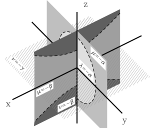
Figure 2: Special surfaces inside ($\lambda=-\alpha$) and outside ($\mu=-\alpha$) the focal ellipse in the plane $x=0$, and inside ($\mu=-\beta$) and outside ($\nu=-\beta$) the two branches of the focal hyperbola in the plane $y=0$ and the plane $z=0$ ($\nu=-\gamma$).

We saw in §2.2 that the velocity ellipsoid is everywhere aligned with the confocal ellipsoidal coordinates. When $\lambda\to-\alpha$, the ellipsoidal coordinate surface degenerates into the area inside the focal ellipse (Fig. 2). The area outside the focal ellipse is labeled by $\mu=-\alpha$. Hence, $T_{\lambda\lambda}$ is perpendicular to the surface inside and $T_{\mu\mu}$ is perpendicular to the surface outside the focal ellipse. On the focal ellipse, i.e. when $\lambda=\mu=-\alpha$, both stress components therefore have to be equal. Similarly, $T_{\mu\mu}$ and $T_{\nu\nu}$ are perpendicular to the area inside ($\mu=-\beta$) and outside ($\nu=-\beta$) the two branches of the focal hyperbola, respectively, and have to be equal on the focal hyperbola itself ($\mu=\nu=-\beta$). This results in the following two continuity conditions

$$T_{\lambda\lambda}(-\alpha,-\alpha,\nu)=T_{\mu\mu}(-\alpha,-\alpha,\nu),$$ (2.17a)

$$T_{\mu\mu}(\lambda,-\beta,-\beta)=T_{\nu\nu}(\lambda,-\beta,-\beta).$$ (2.17b)

These conditions not only follow from geometrical arguments, but are also precisely the conditions necessary to avoid singularities in the Jeans equations (2.16) when $\lambda=\mu=-\alpha$ and $\mu=\nu=-\beta$. For the sake of physical understanding, we will also obtain the corresponding continuity conditions by geometrical arguments for the limiting cases that follow.

2.5 Limiting cases

When two or all three of the constants $\alpha$, $\beta$ or $\gamma$ are equal, the triaxial Stäckel models reduce to limiting cases with more symmetry and thus with fewer degrees of freedom. We show in §2.6 that solving the Jeans equations for all the models with two degrees of freedom reduces to the same two-dimensional problem. EL89 first solved this generalised problem and applied it to the disc, oblate and prolate case. Evans et al. (2000) showed that the large radii case with scale-free DF reduces to the problem solved by EL89. We solve the same problem in a different way in §3, and obtain a simpler expression than EL89. In order to make application of the resulting solution straightforward, and to define a unified notation, we first give an overview of the limiting cases.

2.5.1 Oblate spheroidal coordinates: prolate potentials

When $\gamma=\beta$, the coordinate surfaces for constant $\lambda$ and $\mu$ reduce to oblate spheroids and hyperboloids of revolution around the $x$-axis. Since the range of $\nu$ is zero, it cannot be used as a coordinate. The hyperboloids of two sheets are now planes containing the $x$-axis. We label these planes by an azimuthal angle $\chi$, defined as $\tan\chi=z/y$. In these oblate spheroidal coordinates ($\lambda,\mu,\chi$) the potential $V_{S}$ has the form (cf. Lynden–Bell 1962b)

$$V_{S}=-\frac{f(\lambda)-f(\mu)}{\lambda\!-\!\mu}-\frac{g(\chi)}{(\lambda+\beta)(\mu+\beta)},$$ (2.18)

where the function $g(\chi)$ is arbitrary, and $f(\tau)=(\tau+\alpha)G(\tau)$, with $G(\tau)$ as in eq. (2.4). The denominator of the second term is proportional to $y^{2}+z^{2}$, so that these potentials are singular along the entire $x$-axis unless $g(\chi)\equiv 0$. In this case, the potential is prolate axisymmetric, and the associated density $\rho_{S}$ is generally prolate as well (de Zeeuw et al.  1986).

The Jeans equations (2.16) reduce to

$$\frac{\partial T_{\lambda\lambda}}{\partial\lambda}+\frac{T_{\lambda\lambda}-T_{\mu\mu}}{2(\lambda-\mu)}+\frac{T_{\lambda\lambda}-T_{\chi\chi}}{2(\lambda+\beta)} = -\rho\frac{\partial V_{S}}{\partial\lambda},$$

$$\frac{\partial T_{\mu\mu}}{\partial\mu}+\frac{T_{\mu\mu}-T_{\lambda\lambda}}{2(\mu-\lambda)}+\frac{T_{\mu\mu}-T_{\chi\chi}}{2(\mu+\beta)} = -\rho\frac{\partial V_{S}}{\partial\mu},$$ (2.19)

$$\frac{\partial T_{\chi\chi}}{\partial\chi} = -\rho\frac{\partial V_{S}}{\partial\chi}.$$

The continuity condition (2.17a) still holds, except that the focal ellipse has become a focal circle. For $\mu=-\beta$, the one-sheeted hyperboloid degenerates into the $x$-axis, so that $T_{\mu\mu}$ is perpendicular to the $x$-axis and coincides with $T_{\chi\chi}$. This gives the following two continuity conditions

$$T_{\lambda\lambda}(-\alpha,-\alpha,\chi) = T_{\mu\mu}(-\alpha,-\alpha,\chi),$$

$$T_{\mu\mu}(\lambda,-\beta,\chi) = T_{\chi\chi}(\lambda,-\beta,\chi).$$

By integrating along characteristics, Hunter et al. (1990) obtained the solution of (2.5.1) for the special prolate models in which only the thin I- and O-tube orbits are populated, so that $T_{\mu\mu}\equiv 0$ and $T_{\lambda\lambda}\equiv 0$, respectively (cf. §2.5.6).

2.5.2 Prolate spheroidal coordinates: oblate potentials

When $\beta=\alpha$, we cannot use $\mu$ as a coordinate and replace it by the azimuthal angle $\phi$, defined as $\tan\phi=y/x$. Surfaces of constant $\lambda$ and $\nu$ are confocal prolate spheroids and two-sheeted hyperboloids of revolution around the $z$-axis. The prolate spheroidal coordinates ($\lambda,\phi,\nu$) follow from the oblate spheroidal coordinates ($\lambda,\mu,\chi$) by taking $\mu\!\to\!\nu$, $\chi\!\to\!\phi$ and $\beta\!\to\!\alpha\!\to\!\gamma$. The potential $V_{S}(\lambda,\phi,\nu)$ is (cf. Lynden–Bell 1962b)

$$V_{S}=-\frac{f(\lambda)-f(\nu)}{\lambda\!-\!\nu}-\frac{g(\phi)}{(\lambda+\alpha)(\nu+\alpha)}.$$ (2.21)

In this case, the denominator of the second term is proportional to $R^{2}=x^{2}+y^{2}$, so that the potential is singular along the entire $z$-axis, unless $g(\phi)$ vanishes. When $g(\phi)\equiv 0$, the potential is oblate, and the same is generally true for the associated density $\rho_{S}$.

The Jeans equations (2.16) reduce to

$$\frac{\partial T_{\lambda\lambda}}{\partial\lambda}+\frac{T_{\lambda\lambda}-T_{\phi\phi}}{2(\lambda+\alpha)}+\frac{T_{\lambda\lambda}-T_{\nu\nu}}{2(\lambda-\nu)} = -\rho\frac{\partial V_{S}}{\partial\lambda},$$

$$\frac{\partial T_{\phi\phi}}{\partial\phi} = -\rho\frac{\partial V_{S}}{\partial\phi}.$$ (2.22)

$$\frac{\partial T_{\nu\nu}}{\partial\nu}+\frac{T_{\nu\nu}-T_{\lambda\lambda}}{2(\nu-\lambda)}+\frac{T_{\nu\nu}-T_{\phi\phi}}{2(\nu+\alpha)} = -\rho\frac{\partial V_{S}}{\partial\nu}.$$

For $\lambda=-\alpha$, the prolate spheroidal coordinate surfaces reduce to the part of the $z$-axis between the foci. The part beyond the foci is reached if $\nu=-\alpha$. Hence, in this case, $T_{\lambda\lambda}$ is perpendicular to part of the $z$-axis between, and $T_{\nu\nu}$ is perpendicular to the part of the $z$-axis beyond the foci. They coincide at the foci ($\lambda=\nu=-\alpha$), resulting in one continuity condition. Two more follow from the fact that $T_{\phi\phi}$ is perpendicular to the (complete) $z$-axis, and thus coincides with $T_{\lambda\lambda}$ and $T_{\nu\nu}$ on the part between and beyond the foci, respectively:

$$T_{\lambda\lambda}(-\alpha,\phi,-\alpha) = T_{\nu\nu}(-\alpha,\phi,-\alpha),$$

$$T_{\lambda\lambda}(-\alpha,\phi,\nu) = T_{\phi\phi}(-\alpha,\phi,\nu),$$ (2.23)

$$T_{\nu\nu}(\lambda,\phi,-\alpha) = T_{\phi\phi}(\lambda,\phi,-\alpha).$$

For oblate models with thin S-tube orbits ($T_{\lambda\lambda}\equiv 0$, see §2.5.6), the analytical solution of (2.5.2) was derived by Bishop (1987) and by de Zeeuw & Hunter (1990). Robijn & de Zeeuw (1996) obtained the second-order velocity moments for models in which the thin tube orbits were thickened iteratively. Dejonghe & de Zeeuw (1988, Appendix D) found a general solution by integrating along characteristics. Evans (1990) gave an algorithm for solving (2.5.2) numerically, and Arnold (1995) computed a solution using characteristics without assuming a separable potential.

2.5.3 Confocal elliptic coordinates: non-circular discs

In the principal plane $z=0$, the ellipsoidal coordinates reduce to confocal elliptic coordinates ($\lambda,\mu$), with coordinate curves that are ellipses ($\lambda$) and hyperbolae ($\mu$), that share their foci on the symmetry $y$-axis. The potential of the perfect elliptic disc, with its surface density distribution stratified on concentric ellipses in the plane $z=0$ ($\nu=-\gamma$), is of Stäckel form both in and outside this plane. By a superposition of perfect elliptic discs, one can construct other surface densities and corresponding disc potentials that are of Stäckel form in the plane $z=0$, but not necessarily outside it (Evans & de Zeeuw 1992). The expression for the potential in the disc is of the form (2.18) with $g(\chi)\equiv 0$:

$$V_{S}=-\frac{f(\lambda)-f(\mu)}{\lambda\!-\!\mu},$$ (2.24)

where again $f(\tau)=(\tau+\alpha)G(\tau)$, so that $G(\tau)$ equals the potential along the $y$-axis.

Omitting all terms with $\nu$ in (2.16), we obtain the Jeans equations for non-circular Stäckel discs

$$\frac{\partial T_{\lambda\lambda}}{\partial\lambda}+\frac{T_{\lambda\lambda}-T_{\mu\mu}}{2(\lambda-\mu)} = -\rho\frac{\partial V_{S}}{\partial\lambda},$$

$$\frac{\partial T_{\mu\mu}}{\partial\mu}+\frac{T_{\mu\mu}-T_{\lambda\lambda}}{2(\mu-\lambda)} = -\rho\frac{\partial V_{S}}{\partial\mu},$$

where now $\rho$ denotes a surface density. The parts of the $y$-axis between and beyond the foci are labeled by $\lambda=-\alpha$ and $\mu=-\alpha$, resulting in the continuity condition

$$T_{\lambda\lambda}(-\alpha,-\alpha)=T_{\mu\mu}(-\alpha,-\alpha).$$ (2.26)

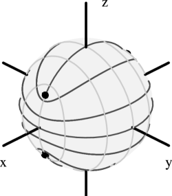
Figure 3: Behaviour of the confocal ellipsoidal coordinates in the limit of large radii $r$. The surfaces of constant $\lambda$ become spheres. The hyperboloids of constant $\mu$ and $\nu$ approach their asymptotic surfaces, and intersect the sphere on the light and dark curves, respectively. These form an orthogonal curvilinear coordinate system $(\mu,\nu)$ on the sphere. The black dots indicate the transition points ($\mu=\nu=-\beta$) between both sets of curves.

2.5.4 Conical coordinates: scale-free triaxial limit

At large radii, the confocal ellipsoidal coordinates ($\lambda,\mu,\nu$) reduce to conical coordinates ($r,\mu,\nu$), with $r$ the usual distance to the origin, i.e., $r^{2}=x^{2}+y^{2}+z^{2}$ and $\mu$ and $\nu$ angular coordinates on the sphere (Fig. 3). The potential $V_{S}(r,\mu,\nu)$ is scale-free, and of the form

$$V_{S}=-{\tilde{F}}(r)+\frac{F(\mu)-F(\nu)}{r^{2}(\mu\!-\!\nu)},$$ (2.27)

where ${\tilde{F}}(r)$ is arbitrary, and $F(\tau)=(\tau+\alpha)(\tau+\gamma)G(\tau)$, as in eq. (2.4).

The Jeans equations in conical coordinates follow from the general triaxial case (2.16) by going to large radii. Taking $\lambda\to r^{2}\gg-\alpha\geq\mu,\nu$, the stress components approach each other and we have

$$\frac{T_{\lambda\lambda}-T_{\mu\mu}}{2(\lambda-\mu)},\;\frac{T_{\lambda\lambda}-T_{\nu\nu}}{2(\lambda-\nu)}\sim\frac{1}{r}\to 0,\quad\frac{\partial}{\partial\lambda}\to\frac{1}{2r}\frac{\partial}{\partial\lambda}.$$ (2.28)

Hence, after multiplying (2.16a) by $2r$, the Jeans equations for scale-free Stäckel models are

$$\frac{\partial T_{rr}}{\partial r}+\frac{2T_{rr}-T_{\mu\mu}-T_{\nu\nu}}{r} = -\rho\frac{\partial V_{S}}{\partial r},$$

$$\frac{\partial T_{\mu\mu}}{\partial\mu}+\frac{T_{\mu\mu}-T_{\nu\nu}}{2(\mu-\nu)} = -\rho\frac{\partial V_{S}}{\partial\mu},$$ (2.29)

$$\frac{\partial T_{\nu\nu}}{\partial\nu}+\frac{T_{\nu\nu}-T_{\mu\mu}}{2(\nu-\mu)} = -\rho\frac{\partial V_{S}}{\partial\nu}.$$

The general Jeans equations in conical coordinates, as derived by Evans et al. (2000), reduce to (2.5.4) for vanishing mixed second moments. At the transition points between the curves of constant $\mu$ and $\nu$ ($\mu=\nu=-\beta$), the tensor components $T_{\mu\mu}$ and $T_{\nu\nu}$ coincide, resulting in the continuity condition

$$T_{\lambda\lambda}(r,-\beta,-\beta)=T_{\phi\phi}(r,-\beta,-\beta).$$ (2.30)

2.5.5 One-dimensional limits

There are several additional limiting cases with more symmetry for which the form of $V_{S}$ (Lynden–Bell 1962b) and the associated Jeans equations follow in a straightforward way from the expressions that were given above. We only mention spheres and circular discs.

When $\alpha\!=\!\beta\!=\!\gamma$, the variables $\mu$ and $\nu$ loose their meaning and the ellipsoidal coordinates reduce to spherical coordinates $(r,\theta,\phi)$. A steady-state spherical model without a preferred axis is invariant under a rotation over the angles $\theta$ and $\phi$, so that we are left with only one Jeans equation in $r$, and $T_{\theta\theta}=T_{\phi\phi}$. This equation can readily be obtained from the CBE in spherical coordinates (e.g., Binney & Tremaine 1987). It also follows as a limit from the Jeans equations (2.16) for triaxial Stäckel models or from any of the above two-dimensional limiting cases. Consider for example the Jeans equations in conical coordinates (2.5.4), and take $\mu\to\theta$ and $\nu\to\phi$. The stress components $T_{rr}$ and $T_{\mu\mu}=T_{\nu\nu}=T_{\phi\phi}=T_{\theta\theta}$ depend only $r$, so that we are left with

$$\frac{dT_{rr}}{dr}+\frac{2(T_{rr}-T_{\theta\theta})}{r}=-\rho\frac{dV_{S}}{dr},$$ (2.31)

which is the well-known result for non-rotating spherical systems (Binney & Tremaine 1987).

In a similar way, the one Jeans equation for the circular disc-case follows from, e.g., the first equation of (2.5.3) by taking $\mu=-\alpha$ and replacing $T_{\mu\mu}$ by $T_{\phi\phi}$, where $\phi$ is the azimuthal angle defined in §2.5.2. With $\lambda+\alpha=R^{2}$ this gives

$$\frac{dT_{RR}}{dR}+\frac{T_{RR}-T_{\phi\phi}}{R}=-\rho\frac{dV_{S}}{dR},$$ (2.32)

which may be compared with Binney & Tremaine (1987), their eq. (4.29).

2.5.6 Thin tube orbits

Each of the three tube orbit families in a triaxial Stäckel model consists of a rotation in one of the ellipsoidal coordinates and oscillations in the other two (§2.2). The I-tubes, for example, rotate in $\nu$ and oscillate in $\lambda$ and $\mu$, with turning points $\mu_{1}$, $\mu_{2}$ and $\lambda_{0}$, so that a typical orbit fills the volume

$$-\gamma\leq\nu\leq-\beta,\quad\mu_{1}\leq\mu\leq\mu_{2},\quad-\alpha\leq\lambda\leq\lambda_{0}.$$ (2.33)

When we restrict ourselves to infinitesimally thin I-tubes, i.e., $\mu_{1}=\mu_{2}$, there is no motion in the $\mu$-coordinate. Therefore, the second-order velocity moment in this coordinate is zero, and thus also the corresponding stress component $T_{\mu\mu}^{\mathrm{I}}\equiv 0$. As a result, eq. (2.16b) reduces to an algebraic relation between $T_{\lambda\lambda}^{\mathrm{I}}$ and $T_{\nu\nu}^{\mathrm{I}}$. This relation can be used to eliminate $T_{\nu\nu}^{\mathrm{I}}$ and $T_{\lambda\lambda}^{\mathrm{I}}$ from the remaining Jeans equations (2.16a) and (2.16c) respectively.

HZ92 solved the resulting two first-order PDEs (their Appendix B) and showed that the same result is obtained by direct evaluation of the second-order velocity moments, using the thin I-tube DF. They derived similar solutions for thin O- and S-tubes, for which there is no motion in the $\lambda$-coordinate, so that $T_{\lambda\lambda}^{\mathrm{O}}\equiv 0$ and $T_{\lambda\lambda}^{\mathrm{S}}\equiv 0$, respectively.

In Stäckel discs we have – besides the flat box orbits – only one family of (flat) tube orbits. For infinitesimally thin tube orbits $T_{\lambda\lambda}\equiv 0$, so that the Jeans equations (2.5.3) reduce to two different relations between $T_{\mu\mu}$ and the density and potential. In §3.4.4, we show how this places restrictions on the form of the density and we give the solution for $T_{\mu\mu}$. We also show that the general solution of (2.5.3), which we obtain in §3, contains the thin tube result. The same is true for the triaxial case: the general solution of (2.16), which we derive in §4, contains the three thin tube orbit solutions as special cases (§4.6.6).

2.6 All two-dimensional cases are similar

EL89 showed that the Jeans equations in oblate and prolate spheroidal coordinates, (2.5.1) and (2.5.2), can be transformed to a system that is equivalent to the two Jeans equations (2.5.3) in confocal elliptic coordinates. Evans et al. (2000) arrived at the same two-dimensional form for Stäckel models with a scale-free DF. We introduce a transformation which differs slightly from that of EL89, but has the advantage that it removes the singular denominators in the Jeans equations.

The Jeans equations (2.5.1) for prolate potentials can be simplified by introducing as dependent variables

$$\mathcal{T}_{\tau\tau}(\lambda,\mu)=(\lambda\!+\!\beta)^{\frac{1}{2}}(\mu\!+\!\beta)^{\frac{1}{2}}(T_{\tau\tau}\!-\!T_{\chi\chi}),\quad\tau=\lambda,\mu,$$ (2.34)

so that the first two equations in (2.5.1) transform to

$$\frac{\partial\mathcal{T}_{\lambda\lambda}}{\partial\lambda}\!+\!\frac{\mathcal{T}_{\lambda\lambda}\!-\!\mathcal{T}_{\mu\mu}}{2(\lambda\!-\!\mu)} = -(\lambda\!+\!\beta)^{\frac{1}{2}}(\mu\!+\!\beta)^{\frac{1}{2}}\!\!\biggl{[}\rho\frac{\partial V_{S}}{\partial\lambda}\!+\!\frac{\partial T_{\chi\chi}}{\partial\lambda}\!\biggr{]},$$

$$\frac{\partial\mathcal{T}_{\mu\mu}}{\partial\mu}\!+\!\frac{\mathcal{T}_{\mu\mu}\!-\!\mathcal{T}_{\lambda\lambda}}{2(\mu\!-\!\lambda)} = -(\mu\!+\!\beta)^{\frac{1}{2}}(\lambda\!+\!\beta)^{\frac{1}{2}}\!\!\biggl{[}\rho\frac{\partial V_{S}}{\partial\mu}\!+\!\frac{\partial T_{\chi\chi}}{\partial\mu}\!\biggr{]}.$$

The third Jeans equation (2.5.1) can be integrated in a straightforward fashion to give the $\chi$-dependence of $T_{\chi\chi}$. It is trivially satisfied for prolate models with $g(\chi)\equiv 0$. Hence if, following EL89, we regard $T_{\chi\chi}(\lambda,\mu)$ as a function which can be prescribed, then equations (2.6) have known right hand sides, and are therefore of the same form as those of the disc case (2.5.3). The singular denominator $(\mu+\beta)$ of (2.5.1) has disappeared, and there is a boundary condition

$$\mathcal{T}_{\mu\mu}(\lambda,-\beta)=0,$$ (2.36)

due to the second continuity condition of (2.5.1) and the definition (2.34).

A similar reduction applies for oblate potentials. The middle equation of (2.5.2) can be integrated to give the $\phi$-dependence of $T_{\phi\phi}$, and is trivially satisfied for oblate models. The remaining two equations (2.5.2) transform to

$$\frac{\partial\mathcal{T}_{\lambda\lambda}}{\partial\lambda}\!+\!\frac{\mathcal{T}_{\lambda\lambda}\!-\!\mathcal{T}_{\nu\nu}}{2(\lambda\!-\!\nu)} = -(\lambda\!+\!\alpha)^{\frac{1}{2}}(-\alpha\!-\!\nu)^{\frac{1}{2}}\!\!\biggl{[}\rho\frac{\partial V_{S}}{\partial\lambda}\!+\!\frac{\partial T_{\phi\phi}}{\partial\lambda}\!\!\biggr{]},$$

$$\frac{\partial\mathcal{T}_{\nu\nu}}{\partial\nu}\!+\!\frac{\mathcal{T}_{\nu\nu}\!-\!\mathcal{T}_{\lambda\lambda}}{2(\nu\!-\!\lambda)} = -(-\alpha\!-\!\nu)^{\frac{1}{2}}(\lambda\!+\!\alpha)^{\frac{1}{2}}\!\!\biggl{[}\rho\frac{\partial V_{S}}{\partial\nu}\!+\!\frac{\partial T_{\phi\phi}}{\partial\nu}\!\!\biggr{]},$$

in terms of the dependent variables

$$\mathcal{T}_{\tau\tau}(\lambda,\nu)=(\lambda\!+\!\alpha)^{\frac{1}{2}}(-\alpha\!-\!\nu)^{\frac{1}{2}}(T_{\tau\tau}\!-\!T_{\phi\phi}),\quad\tau=\lambda,\nu.$$ (2.38)

We now have two boundary conditions

$$\mathcal{T}_{\lambda\lambda}(-\alpha,\nu)=0,\quad\mathcal{T}_{\nu\nu}(\lambda,-\alpha)=0,$$ (2.39)

as a consequence of the last two continuity conditions of (2.5.2) and the definitions (2.38).

In the case of a scale-free DF, the stress components in the Jeans equations in conical coordinates (2.5.4) have the form $T_{\tau\tau}=r^{-\zeta}\mathcal{T}_{\tau\tau}(\mu,\nu)$, with $\zeta>0$ and $\tau=r,\mu,\nu$. After substitution and multiplication by $r^{\zeta+1}$, the first equation of (2.5.4) reduces to

$$(2-\zeta)\mathcal{T}_{rr}+\mathcal{T}_{\mu\mu}+\mathcal{T}_{\nu\nu}=r^{\zeta+1}\rho\frac{\partial V_{S}}{\partial r}.$$ (2.40)

When $\zeta=2$, $\mathcal{T}_{rr}$ drops out, so that the relation between $\mathcal{T}_{\mu\mu}$ and $\mathcal{T}_{\nu\nu}$ is known and the remaining two Jeans equations can be readily solved (Evans et al. 2000). In all other cases, $\mathcal{T}_{rr}$ can be obtained from (2.40) once we have solved the last two equations of (2.5.4) for $\mathcal{T}_{\mu\mu}$ and $\mathcal{T}_{\nu\nu}$. This pair of equations is identical to the system of Jeans equations (2.5.3) for the case of disc potentials. The latter is the simplest form of the equivalent two-dimensional problem for all Stäckel models with two degrees of freedom. We solve it in the next section.

Once we have derived the solution of (2.5.3), we may obtain the solution for prolate Stäckel potentials by replacing all terms $-\rho\partial V_{s}/\partial\tau$ $(\tau=\lambda,\mu)$ by the right-hand side of (2.6) and substituting the transformations (2.34) for $T_{\lambda\lambda}$ and $T_{\mu\mu}$. Similarly, our unified notation makes the application of the solution of (2.5.3) to the oblate case and to models with a scale-free DF straightforward (§3.4).

3 The two-dimensional case

We first apply Riemann’s method to solve the Jeans equations (2.5.3) in confocal elliptic coordinates for Stäckel discs (§2.5.3). This involves finding a Riemann–Green function that describes the solution for a source point of stress. The full solution is then obtained in compact form by representing the known right-hand side terms as a sum of sources. In §3.2, we introduce an alternative approach, the singular solution method. Unlike Riemann’s method, this can be extended to the three-dimensional case, as we show in §4. We analyse the choice of the boundary conditions in detail in §3.3. In §3.4, we apply the two-dimensional solution to the axisymmetric and scale-free limits, and we also consider a Stäckel disc built with thin tube orbits.

3.1 Riemann’s method

After differentiating the first Jeans equation of (2.5.3) with respect to $\mu$ and eliminating terms in $T_{\mu\mu}$ by applying the second equation, we obtain a second-order partial differential equation (PDE) for $T_{\lambda\lambda}$ of the form

$$\frac{\partial^{2}T_{\lambda\lambda}}{\partial\lambda\partial\mu}-\frac{3}{2(\lambda\!-\!\mu)}\frac{\partial T_{\lambda\lambda}}{\partial\lambda}+\frac{1}{2(\lambda\!-\!\mu)}\frac{\partial T_{\lambda\lambda}}{\partial\mu}=U_{\lambda\lambda}(\lambda,\mu).$$ (3.1)

Here $U_{\lambda\lambda}$ is a known function given by

$$U_{\lambda\lambda}=-\frac{1}{(\lambda\!-\!\mu)^{\frac{3}{2}}}\frac{\partial}{\partial\mu}\biggl{[}(\lambda\!-\!\mu)^{\frac{3}{2}}\rho\frac{\partial V_{S}}{\partial\lambda}\biggr{]}-\frac{\rho}{2(\lambda\!-\!\mu)}\frac{\partial V_{S}}{\partial\mu}.$$ (3.2)

We obtain a similar second-order PDE for $T_{\mu\mu}$ by interchanging $\lambda\leftrightarrow\mu$. Both PDEs can be solved by Riemann’s method. To solve them simultaneously, we define the linear second-order differential operator

$$\mathcal{L}=\frac{\partial^{2}}{\partial\lambda\partial\mu}-\frac{c_{1}}{\lambda\!-\!\mu}\frac{\partial}{\partial\lambda}+\frac{c_{2}}{\lambda\!-\!\mu}\frac{\partial}{\partial\mu},$$ (3.3)

with $c_{1}$ and $c_{2}$ constants to be specified. Hence, the more general second-order PDE

$$\mathcal{L}\,T=U,$$ (3.4)

with $T$ and $U$ functions of $\lambda$ and $\mu$ alone, reduces to those for the two stress components by taking

$$T=T_{\lambda\lambda}\!\!\!\!\! : c_{1}={\textstyle\frac{3}{2}},\quad c_{2}={\textstyle\frac{1}{2}},\quad U=U_{\lambda\lambda},$$

$$T=T_{\mu\mu}\!\!\!\!\! : c_{1}={\textstyle\frac{1}{2}},\quad c_{2}={\textstyle\frac{3}{2}},\quad U=U_{\mu\mu}.$$

In what follows, we introduce a Riemann–Green function $\mathcal{G}$ and incorporate the left-hand side of (3.4) into a divergence. Green’s theorem then allows us to rewrite the surface integral as a line integral over its closed boundary, which can be evaluated if $\mathcal{G}$ is chosen suitably. We determine the Riemann–Green function $\mathcal{G}$ which satisfies the required conditions, and then construct the solution.

3.1.1 Application of Riemann’s method

We form a divergence by defining a linear operator $\mathcal{L}^{\star}$, called the adjoint of $\mathcal{L}$ (e.g., Copson 1975), as

$$\mathcal{L}^{\star}=\frac{\partial^{2}}{\partial\lambda\partial\mu}+\frac{\partial}{\partial\lambda}\biggl{(}\!\frac{c_{1}}{\lambda\!-\!\mu}\!\biggr{)}-\frac{\partial}{\partial\mu}\biggl{(}\!\frac{c_{2}}{\lambda\!-\!\mu}\!\biggr{)}.$$ (3.6)

The combination $\mathcal{G}\mathcal{L}T-T\mathcal{L}^{\star}\mathcal{G}$ is a divergence for any twice differentiable function $\mathcal{G}$ because

$$\mathcal{G}\mathcal{L}T-T\mathcal{L}^{\star}\mathcal{G}=\partial L/\partial\lambda+\partial M/\partial\mu,$$ (3.7)

where

$$L(\lambda,\mu) = \frac{\mathcal{G}}{2}\frac{\partial T}{\partial\mu}-\frac{T}{2}\frac{\partial\mathcal{G}}{\partial\mu}-\frac{c_{1}\,\mathcal{G}\,T}{\lambda\!-\!\mu},$$

$$M(\lambda,\mu) = \frac{\mathcal{G}}{2}\frac{\partial T}{\partial\lambda}-\frac{T}{2}\frac{\partial\mathcal{G}}{\partial\lambda}+\frac{c_{2}\,\mathcal{G}\,T}{\lambda\!-\!\mu}.$$

We now apply the PDE (3.4) and the definition (3.6) in zero-subscripted variables $\lambda_{0}$ and $\mu_{0}$. We integrate the divergence (3.7) over the domain $D=\{(\lambda_{0},\mu_{0})$: $\lambda\leq\lambda_{0}\leq\infty,\mu\leq\mu_{0}\leq-\alpha\}$, with closed boundary $\Gamma$ (Fig. 4). It follows by Green’s theorem that

$$\iint\limits_{D}{\mathrm{d}}\lambda_{0}{\mathrm{d}}\mu_{0}\Bigl{(}\mathcal{G}\mathcal{L}_{0}T-T\mathcal{L}_{0}^{\star}\mathcal{G}\Bigr{)}=\\[-10.0pt] \oint\limits_{\Gamma}\!{\mathrm{d}}\mu_{0}\,L(\lambda_{0},\mu_{0})-\oint\limits_{\Gamma}\!{\mathrm{d}}\lambda_{0}\,M(\lambda_{0},\mu_{0}),$$ (3.9)

where $\Gamma$ is circumnavigated counter-clockwise. Here $\mathcal{L}_{0}$ and $\mathcal{L}_{0}^{\star}$ denote the operators (3.3) and (3.6) in zero-subscripted variables. We shall seek a Riemann–Green function $\mathcal{G}(\lambda_{0},\mu_{0})$ which solves the PDE

$$\mathcal{L}_{0}^{\star}\mathcal{G}=0,$$ (3.10)

in the interior of $D$. Then the left-hand side of (3.9) becomes $\iint_{D}{\mathrm{d}}\lambda_{0}{\mathrm{d}}\mu_{0}\mathcal{G}(\lambda_{0},\mu_{0})\,U(\lambda_{0},\mu_{0})$. The right-hand side of (3.9) has a contribution from each of the four sides of the rectangular boundary $\Gamma$. We suppose that $M(\lambda_{0},\mu_{0})$ and $L(\lambda_{0},\mu_{0})$ decay sufficiently rapidly as $\lambda_{0}\to\infty$ so that the contribution from the boundary at $\lambda_{0}=\infty$ vanishes and the infinite integration over $\lambda_{0}$ converges. Partial integration of the remaining terms then gives for the boundary integral

$$\int\limits_{\lambda}^{\infty}{\mathrm{d}}\lambda_{0}\Bigl{[}\!\Bigl{(}\frac{\partial\mathcal{G}}{\partial\lambda_{0}}\!-\!\frac{c_{2}\,\mathcal{G}}{\lambda_{0}\!-\!\mu_{0}}\Bigr{)}T\underset{\mu_{0}=\mu}{\Bigr{]}}\!+\!\!\int\limits_{\mu}^{-\alpha}{\mathrm{d}}\mu_{0}\Bigl{[}\Bigl{(}\frac{\partial\mathcal{G}}{\partial\mu_{0}}\!+\!\frac{c_{1}\,\mathcal{G}}{\lambda_{0}\!-\!\mu_{0}}\Bigr{)}T\underset{\lambda_{0}=\lambda}{\Bigr{]}}\\ \!+\!\int\limits_{\lambda}^{\infty}{\mathrm{d}}\lambda_{0}\Bigl{[}\Bigl{(}\frac{\partial T}{\partial\lambda_{0}}\!+\!\frac{c_{2}\,T}{\lambda_{0}\!-\!\mu_{0}}\Bigr{)}\mathcal{G}\underset{\mu_{0}=-\alpha}{\Bigr{]}}+\,\mathcal{G}(\lambda,\mu)T(\lambda,\mu).$$ (3.11)

We now impose on $\mathcal{G}$ the additional conditions

$$\mathcal{G}(\lambda,\mu)=1,$$ (3.12)

and

$$\frac{\partial\mathcal{G}}{\partial\lambda_{0}}-\frac{c_{2}\,\mathcal{G}}{\lambda_{0}\!-\!\mu_{0}}=0\qquad \mathrm{on} \quad\mu_{0}=\mu,$$

$$\frac{\partial\mathcal{G}}{\partial\mu_{0}}+\frac{c_{1}\,\mathcal{G}}{\lambda_{0}\!-\!\mu_{0}}=0\qquad \mathrm{on} \quad\lambda_{0}=\lambda.$$

Then eq. (3.9) gives the explicit solution

$$T(\lambda,\mu)=\int\limits_{\lambda}^{\infty}{\mathrm{d}}\lambda_{0}\int\limits_{\mu}^{-\alpha}{\mathrm{d}}\mu_{0}\,\mathcal{G}(\lambda_{0},\mu_{0})\,U(\lambda_{0},\mu_{0})\\[-10.0pt] -\int\limits_{\lambda}^{\infty}{\mathrm{d}}\lambda_{0}\Bigl{[}\Bigl{(}\frac{\partial T}{\partial\lambda_{0}}\!+\!\frac{c_{2}\,T}{\lambda_{0}\!-\!\mu_{0}}\Bigr{)}\mathcal{G}\underset{\mu_{0}=-\alpha}{\Bigr{]}}\hskip 10.0pt,$$ (3.14)

for the stress component, once we have found the Riemann–Green function $\mathcal{G}$.

Figure 4: The $(\lambda_{0},\mu_{0})$-plane. The total stress at a field point $(\lambda,\mu)$, consists of the weighted contributions from source points at $(\lambda_{0},\mu_{0})$ in the domain $D$, with boundary $\Gamma$.

3.1.2 The Riemann–Green function

Our prescription for the Riemann–Green function $\mathcal{G}(\lambda_{0},\mu_{0})$ is that it satisfies the PDE (3.10) as a function of $\lambda_{0}$ and $\mu_{0}$, and that it satisfies the boundary conditions (3.12) and (3.1.1) at the specific values $\lambda_{0}=\lambda$ and $\mu_{0}=\mu$. Consequently $\mathcal{G}$ depends on two sets of coordinates. Henceforth, we denote it as $\mathcal{G}(\lambda,\mu;\lambda_{0},\mu_{0})$.

An explicit expression for the Riemann–Green function which solves (3.10) is (Copson 1975)

$$\mathcal{G}(\lambda,\mu;\lambda_{0},\mu_{0})=\frac{(\lambda_{0}\!-\!\mu_{0})^{c_{2}}(\lambda\!-\!\mu_{0})^{c_{1}-c_{2}}}{(\lambda\!-\!\mu)^{c_{1}}}F(w),$$ (3.15)

where the parameter $w$ is defined as

$$w=\frac{(\lambda_{0}\!-\!\lambda)(\mu_{0}\!-\!\mu)}{(\lambda_{0}\!-\!\mu_{0})(\lambda\!-\!\mu)},$$ (3.16)

and $F(w)$ is to be determined. Since $w=0$ when $\lambda_{0}=\lambda$ or $\mu_{0}=\mu$, it follows from (3.12) that the function $F$ has to satisfy $F(0)=1$. It is straightforward to verify that $\mathcal{G}$ satisfies the conditions (3.1.1), and that eq. (3.10) reduces to the following ordinary differential equation for $F(w)$

$$w(1\!-\!w)F^{\prime\prime}+[1\!-\!(2+c_{1}\!-\!c_{2})w]F^{\prime}-c_{1}(1\!-\!c_{2})F=0.$$ (3.17)

This is a hypergeometric equation (e.g., Abramowitz & Stegun 1965), and its unique solution satisfying $F(0)=1$ is

$$F(w)={}_{2}F_{1}(c_{1},1\!-\!c_{2};1;w).$$ (3.18)

The Riemann–Green function (3.15) represents the influence at a field point at $(\lambda,\mu)$ due to a source point at $(\lambda_{0},\mu_{0})$. Hence it satisfies the PDE

$$\mathcal{L}\,\mathcal{G}(\lambda,\mu;\lambda_{0},\mu_{0})=\delta(\lambda_{0}\!-\!\lambda)\delta(\mu_{0}\!-\!\mu).$$ (3.19)

The first right-hand side term of the solution (3.14) is a sum over the sources in $D$ which are due to the inhomogeneous term $U$ in the PDE (3.4). That PDE is hyperbolic with characteristic variables $\lambda$ and $\mu$. By choosing to apply Green’s theorem to the domain $D$, we made it the domain of dependence (Strauss 1992) of the field point $(\lambda,\mu)$ for (3.4), and hence we implicitly decided to integrate that PDE in the direction of decreasing $\lambda$ and decreasing $\mu$.

The second right-hand side term of the solution (3.14) represents the solution to the homogeneous PDE $\mathcal{L}\,T=0$ due to the boundary values of $T$ on the part of the boundary $\mu=-\alpha$ which lies within the domain of dependence. There is only one boundary term because we implicitly require that $T(\lambda,\mu)\to 0$ as $\lambda\to\infty$. We verify in §3.1.4 that this requirement is indeed satisfied.

3.1.3 The disc solution

We obtain the Riemann–Green functions for $T_{\lambda\lambda}$ and $T_{\mu\mu}$, labeled as $\mathcal{G}_{\lambda\lambda}$ and $\mathcal{G}_{\mu\mu}$, respectively, from expressions (3.15) and (3.18) by substitution of the values for the constants $c_{1}$ and $c_{2}$ from (3.1). The hypergeometric function in $\mathcal{G}_{\lambda\lambda}$ is the complete elliptic integral of the second kind, $E(w)$. The hypergeometric function in $\mathcal{G}_{\mu\mu}$ can also be expressed in terms of $E(w)$ using eq. (15.2.15) of Abramowitz & Stegun (1965), so that we can write

$$\mathcal{G}_{\lambda\lambda}(\lambda,\mu;\lambda_{0},\mu_{0})=\frac{(\lambda_{0}\!-\!\mu_{0})^{\frac{3}{2}}}{(\lambda\!-\!\mu)^{\frac{1}{2}}}\frac{2E(w)}{\pi(\lambda_{0}\!-\!\mu)},$$ (3.20a)

$$\mathcal{G}_{\mu\mu}(\lambda,\mu;\lambda_{0},\mu_{0})=\frac{(\lambda_{0}\!-\!\mu_{0})^{\frac{3}{2}}}{(\lambda\!-\!\mu)^{\frac{1}{2}}}\frac{2E(w)}{\pi(\lambda\!-\!\mu_{0})},$$ (3.20b)

Substituting these into (3.14) gives the solution of the stress components throughout the disc as

$$T_{\lambda\lambda}(\lambda,\mu)=\frac{2}{\pi(\lambda\!-\!\mu)^{\frac{1}{2}}}\Biggl{\{}\\ \int\limits_{\lambda}^{\infty}{\mathrm{d}}\lambda_{0}\int\limits_{\mu}^{-\alpha}{\mathrm{d}}\mu_{0}\!\frac{E(w)}{(\lambda_{0}\!\!-\!\mu)}\!\biggl{\{}\!\!\frac{\partial}{\partial\mu_{0}}\!\biggl{[}\!-(\lambda_{0}\!-\!\mu_{0})^{\frac{3}{2}}\!\rho\frac{\partial V_{S}}{\partial\lambda_{0}}\!\biggr{]}\!-\frac{(\lambda_{0}\!\!-\!\mu_{0})^{\frac{1}{2}}}{2}\!\rho\frac{\partial V_{S}}{\partial\mu_{0}}\!\biggr{\}}\\ -\!\!\int\limits_{\lambda}^{\infty}{\mathrm{d}}\lambda_{0}\biggl{[}\!\frac{E(w)}{(\lambda_{0}\!-\!\mu)}\underset{\mu_{0}=-\alpha}{\biggr{]}}(\lambda_{0}\!+\!\alpha)\frac{{\mathrm{d}}}{{\mathrm{d}}\lambda_{0}}\!\Bigl{[}\!(\lambda_{0}\!+\!\alpha)^{\frac{1}{2}}T_{\lambda\lambda}(\lambda_{0},-\alpha)\!\Bigr{]}\!\!\Biggr{\}},$$ (3.21a)

$$T_{\mu\mu}(\lambda,\mu)=\frac{2}{\pi(\lambda\!-\!\mu)^{\frac{1}{2}}}\Biggl{\{}\\ \int\limits_{\lambda}^{\infty}{\mathrm{d}}\lambda_{0}\int\limits_{\mu}^{-\alpha}{\mathrm{d}}\mu_{0}\!\frac{E(w)}{(\lambda\!-\!\mu_{0})}\!\biggl{\{}\!\!\frac{\partial}{\partial\lambda_{0}}\!\biggl{[}\!-(\lambda_{0}\!-\!\mu_{0})^{\frac{3}{2}}\!\rho\frac{\partial V_{S}}{\partial\mu_{0}}\!\biggr{]}\!+\frac{(\lambda_{0}\!\!-\!\mu_{0})^{\frac{1}{2}}}{2}\!\rho\frac{\partial V_{S}}{\partial\lambda_{0}}\!\biggr{\}}\\ -\!\!\int\limits_{\lambda}^{\infty}{\mathrm{d}}\lambda_{0}\,\biggl{[}\!\frac{E(w)}{(\lambda\!-\!\mu_{0})}\underset{\mu_{0}=-\alpha}{\biggr{]}}\frac{{\mathrm{d}}}{{\mathrm{d}}\lambda_{0}}\!\Bigl{[}\!(\lambda_{0}\!+\!\alpha)^{\frac{3}{2}}T_{\mu\mu}(\lambda_{0},-\alpha)\!\Big{]}\!\!\Biggr{\}}.$$ (3.21b)

This solution depends on $\rho$ and $V_{S}$, which are assumed to be known, and on $T_{\lambda\lambda}(\lambda,-\alpha)$ and $T_{\mu\mu}(\lambda,-\alpha)$, i.e., the stress components on the part of the $y$-axis beyond the foci. Because these two stress components satisfy the first Jeans equation of (2.5.3) at $\mu=-\alpha$, we are only free to choose one of them, say $T_{\mu\mu}(\lambda,-\alpha)$. $T_{\lambda\lambda}(\lambda,-\alpha)$ then follows by integrating this first Jeans equation with respect to $\lambda$, using the continuity condition (2.26) and requiring that $T_{\lambda\lambda}(\lambda,-\alpha)\to 0$ as $\lambda\to\infty$.

3.1.4 Consistency check

We now investigate the behaviour of our solutions at large distances and verify that our working hypothesis concerning the radial fall-off of the functions $L$ and $M$ in eq. (3.1.1) is correct. The solution (3.14) consists of two components: an area integral due to the inhomogeneous right-hand side term of the PDE (3.4), and a single integral due to the boundary values. We examine them in turn to obtain the conditions for the integrals to converge. Next, we parameterise the behaviour of the density and potential at large distances and apply it to the solution (3.21) and to the energy equation (2.10) to check if the convergence conditions are satisfied for physical potential-density pairs.

As $\lambda_{0}\to\infty$, $w$ tends to the finite limit $(\mu_{0}-\mu)/(\lambda-\mu)$. Hence $E(w)$ is finite, and so, by (3.20), $\mathcal{G}_{\lambda\lambda}=\mathcal{O}(\lambda_{0}^{1/2})$ and $\mathcal{G}_{\mu\mu}=\mathcal{O}(\lambda_{0}^{3/2})$. Suppose now that $U_{\lambda\lambda}(\lambda_{0},\mu_{0})=\mathcal{O}(\lambda_{0}^{-l_{1}-1})$ and $U_{\mu\mu}(\lambda_{0},\mu_{0})=\mathcal{O}(\lambda_{0}^{-m_{1}-1})$ as $\lambda_{0}\to\infty$. The area integrals in the solution (3.14) then converge, provided that $l_{1}>\frac{1}{2}$ and $m_{1}>\frac{3}{2}$. These requirements place restrictions on the behaviour of the density $\rho$ and potential $V_{S}$ which we examine below. Since $\mathcal{G}_{\lambda\lambda}(\lambda,\mu;\lambda_{0},\mu_{0})$ is $\mathcal{O}(\lambda^{-1/2})$ as $\lambda\to\infty$, the area integral component of $T_{\lambda\lambda}(\lambda,\mu)$ behaves as $\mathcal{O}(\lambda^{-1/2}\int_{\lambda}^{\infty}\lambda_{0}^{-l_{1}-1/2}d\lambda_{0})$ and so is $\mathcal{O}(\lambda^{-l_{1}})$. Similarly, with $\mathcal{G}_{\mu\mu}(\lambda,\mu;\lambda_{0},\mu_{0})=\mathcal{O}(\lambda^{-3/2})$ as $\lambda\to\infty$, the first component of $T_{\mu\mu}(\lambda,\mu)$ is $\mathcal{O}(\lambda_{0}^{-m_{1}})$.

To analyse the second component of the solution (3.14), we suppose that the boundary value $T_{\lambda\lambda}(\lambda_{0},-\alpha)=\mathcal{O}(\lambda_{0}^{-l_{2}})$ and $T_{\mu\mu}(\lambda_{0},-\alpha)=\mathcal{O}(\lambda_{0}^{-m_{2}})$ as $\lambda_{0}\to\infty$. A similar analysis then shows that the boundary integrals converge, provided that $l_{2}>\frac{1}{2}$ and $m_{2}>\frac{3}{2}$, and that the second components of $T_{\lambda\lambda}(\lambda,\mu)$ and $T_{\mu\mu}(\lambda,\mu)$ are $\mathcal{O}(\lambda^{-l_{2}})$ and $\mathcal{O}(\lambda^{-m_{2}})$ as $\lambda\to\infty$, respectively.

We conclude that the convergence of the integrals in the solution (3.14) requires that $T_{\lambda\lambda}(\lambda,\mu)$ and $T_{\mu\mu}(\lambda,\mu)$ decay at large distance as $\mathcal{O}(\lambda^{-l})$ with $l>\frac{1}{2}$ and $\mathcal{O}(\lambda^{-m})$ with $m>\frac{3}{2}$, respectively. The requirements which we have imposed on $U(\lambda_{0},\mu_{0})$ and $T(\lambda_{0},-\alpha)$ cause the contributions to $\oint_{\Gamma}d\mu_{0}L(\lambda_{0},\mu_{0})$ in Green’s formula (3.9) from the segment of the path at large $\lambda_{0}$ to be negligible in all cases.

Having obtained the requirements for the Riemann–Green function analysis to be valid, we now investigate the circumstances in which they apply. Following Arnold et al. (1994), we consider densities $\rho$ that decay as $N(\mu)\lambda^{-s/2}$ at large distances. We suppose that the function $G(\tau)$ introduced in eq. (2.4) is $\mathcal{O}(\tau^{\delta})$ for $-\frac{1}{2}\leq\delta<0$ as $\tau\to\infty$. The lower limit $\delta=-\frac{1}{2}$ corresponds to a potential due to a finite total mass, while the upper limit restricts it to potentials that decay to zero at large distances.

For the disc potential (2.24), we then have that $f(\tau)=\mathcal{O}(\tau^{\delta+1})$ when $\tau\to\infty$. Using the definition (3.2), we obtain

$$U_{\lambda\lambda}(\lambda,\mu)=\frac{f^{\prime}(\mu)-f^{\prime}(\lambda)}{2(\lambda-\mu)^{2}}\rho+\frac{V_{S}+f^{\prime}(\lambda)}{(\lambda-\mu)}\frac{\partial\rho}{\partial\mu},$$ (3.22a)

$$U_{\mu\mu}(\lambda,\mu)=\frac{f^{\prime}(\lambda)-f^{\prime}(\mu)}{2(\lambda-\mu)^{2}}\rho-\frac{V_{S}+f^{\prime}(\mu)}{(\lambda-\mu)}\frac{\partial\rho}{\partial\lambda},$$ (3.22b)

where $\rho$ is the surface density of the disc. It follows that $U_{\lambda\lambda}(\lambda,\mu)$ is generally the larger and is $\mathcal{O}(\lambda^{\delta-s/2-1})$ as $\lambda\to\infty$, whereas $U_{\mu\mu}(\lambda,\mu)$ is $\mathcal{O}(\lambda^{-2-s/2})$. Hence, for the components of the stresses (3.21) we have $T_{\lambda\lambda}=\mathcal{O}(\lambda^{\delta-s/2})$ and $T_{\mu\mu}=\mathcal{O}(\lambda^{-1-s/2})$. This estimate for $U_{\lambda\lambda}$ assumes that $\partial\rho/\partial\mu$ is also $\mathcal{O}(\lambda^{-s/2})$. It is too high if the density becomes independent of angle at large distances, as it does for discs with $s<3$ (Evans & de Zeeuw 1992). Using these estimates with the requirements for integral convergence that were obtained earlier, we obtain the conditions $s>2\delta+1$ and $s>1$, respectively, for inhomogeneous terms in $T_{\lambda\lambda}(\lambda,\mu)$ and $T_{\mu\mu}(\lambda,\mu)$ to be valid solutions. The second condition implies the first because $\delta<0$.

With $V_{S}(\lambda,\mu)=\mathcal{O}(\lambda^{\delta})$ at large $\lambda$, it follows from the energy equation (2.10) for bound orbits that the second-order velocity moments $\langle v_{\tau}^{2}\rangle$ cannot exceed $\mathcal{O}(\lambda^{\delta})$, and hence that stresses $T_{\tau\tau}=\rho\langle v_{\tau}^{2}\rangle$ cannot exceed $\mathcal{O}(\lambda^{\delta-s/2})$. This implies for $T_{\lambda\lambda}(\lambda,\mu)$ that $s>2\delta+1$, and for $T_{\mu\mu}(\lambda,\mu)$ we have the more stringent requirement that $s>2\delta+3$. This last requirement is unnecessarily restrictive, but an alternative form of the solution is needed to do better. Since that alternative form arises naturally with the singular solution method, we return to this issue in §3.2.6.

Thus, for the Riemann–Green solution to apply, we find the conditions $s>1$ and $-\frac{1}{2}\leq\delta<0$. These conditions are satisfied for the perfect elliptic disk $(s=3,\delta=-\frac{1}{2})$, and for many other separable discs (Evans & de Zeeuw 1992).

3.1.5 Relation to the EL89 analysis

EL89 solve for the difference $\Delta\equiv T_{\lambda\lambda}-T_{\mu\mu}$ using a Green’s function method which is essentially equivalent to the approach used here. EL89 give the Fourier transform of their Green’s function, but do not invert it. We give the Riemann–Green function for $\Delta$ in Appendix A, and then rederive it by a Laplace transform analysis. Our Laplace transform analysis can be recast in terms of Fourier transforms. When we do this, we obtain a result which differs from that of EL89.

3.2 Singular Solution Superposition

We have solved the disc problem (2.5.3) by combining the two Jeans equations into a single second-order PDE in one of the stress components, and then applying Riemann’s method to it. However, Riemann’s method and other standard techniques do not carry over to a single third-order PDE in one dependent variable, which is the best that one could expect to have in the general case. We therefore introduce an alternative but equivalent method of solution, also based on the superposition of source points. In constrast to Riemann’s method, this singular solution method is applicable to the general case of triaxial Stäckel models.

3.2.1 Simplified Jeans equations

We define new independent variables

$$S_{\lambda\lambda}(\lambda,\mu) = |\lambda\!-\!\mu|^{\frac{1}{2}}\,T_{\lambda\lambda}(\lambda,\mu),$$

$$S_{\mu\mu}(\lambda,\mu) = |\mu\!-\!\lambda|^{\frac{1}{2}}\,T_{\mu\mu}(\lambda,\mu),$$

where $|.|$ denotes absolute value, introduced to make the square root single-valued with respect to cyclic permutation of $\lambda\to\mu\to\lambda$. The Jeans equations (2.5.3) can then be written in the form

$$\frac{\partial S_{\lambda\lambda}}{\partial\lambda}-\frac{S_{\mu\mu}}{2(\lambda\!-\!\mu)}=-|\lambda\!-\!\mu|^{\frac{1}{2}}\rho\frac{\partial V_{S}}{\partial\lambda}\equiv g_{1}(\lambda,\mu),$$ (3.24a)

$$\frac{\partial S_{\mu\mu}}{\partial\mu}-\frac{S_{\lambda\lambda}}{2(\mu\!-\!\lambda)}=-|\mu\!-\!\lambda|^{\frac{1}{2}}\rho\frac{\partial V_{S}}{\partial\mu}\equiv g_{2}(\lambda,\mu).$$ (3.24b)

For given density and potential, $g_{1}$ and $g_{2}$ are known functions of $\lambda$ and $\mu$. Next, we consider a simplified form of (3.24) by taking for $g_{1}$ and $g_{2}$, respectively

$$\tilde{g}_{1}(\lambda,\mu)=0,\quad\tilde{g}_{2}(\lambda,\mu)=\delta(\lambda_{0}\!-\!\lambda)\delta(\mu_{0}\!-\!\mu),$$ (3.25)

with $-\beta\leq\mu\leq\mu_{0}\leq-\alpha\leq\lambda\leq\lambda_{0}$. A similar set of simplified equations is obtained by interchanging the expressions for $\tilde{g}_{1}$ and $\tilde{g}_{2}$. We refer to solutions of these simplified Jeans equations as singular solutions.

Singular solutions can be interpreted as contributions to the stresses at a fixed point $(\lambda,\mu)$ due to a source point in $(\lambda_{0},\mu_{0})$ (Fig. 4). The full stress at the field point can be obtained by adding all source point contributions, each with a weight that depends on the local density and potential. In what follows, we derive the singular solutions, and then use this superposition principle to construct the solution for the Stäckel discs in §3.2.6.

3.2.2 Homogeneous boundary problem

The choice (3.25) places constraints on the functional form of $S_{\lambda\lambda}$ and $S_{\mu\mu}$. The presence of the delta-functions in $\tilde{g}_{2}$ requires that $S_{\mu\mu}$ contains a term $-\delta(\lambda_{0}\!-\!\lambda)\mathcal{H}(\mu_{0}\!-\!\mu)$, with the step-function

$$\mathcal{H}(x\!-\!x_{0})=\begin{cases}0,&\text{$x<x_{0}$},\\ 1,&\text{$x\geq x_{0}$}.\end{cases}$$ (3.26)

Since $\mathcal{H}^{\prime}(y)=\delta(y)$, it follows that, by taking the partial derivative of $-\delta(\lambda_{0}\!-\!\lambda)\mathcal{H}(\mu_{0}\!-\!\mu)$ with respect to $\mu$, the delta-functions are balanced. There is no balance when $S_{\lambda\lambda}$ contains $\delta(\lambda_{0}\!-\!\lambda)$, and similarly neither stress components can contain $\delta(\mu_{0}\!-\!\mu)$. We can, however, add a function of $\lambda$ and $\mu$ to both components, multiplied by $\mathcal{H}(\lambda_{0}\!-\!\lambda)\mathcal{H}(\mu_{0}\!-\!\mu)$. In this way, we obtain a singular solution of the form

$$S_{\lambda\lambda} = A(\lambda,\mu)\mathcal{H}(\lambda_{0}\!-\!\lambda)\mathcal{H}(\mu_{0}\!-\!\mu),$$

$$S_{\mu\mu} = B(\lambda,\mu)\mathcal{H}(\lambda_{0}\!-\!\lambda)\mathcal{H}(\mu_{0}\!-\!\mu)\!-\!\delta(\lambda_{0}\!-\!\lambda)\mathcal{H}(\mu_{0}\!-\!\mu),$$

in terms of functions $A$ and $B$ that have to be determined. Substituting these forms in the simplified Jeans equations and matching terms yields two homogeneous equations

$$\frac{\partial A}{\partial\lambda}-\frac{B}{2(\lambda\!-\!\mu)}=0,\quad\frac{\partial B}{\partial\mu}-\frac{A}{2(\mu\!-\!\lambda)}=0,$$ (3.28)

and two boundary conditions

$$A(\lambda_{0},\mu)=\frac{1}{2(\lambda_{0}\!-\!\mu)},\quad B(\lambda,\mu_{0})=0.$$ (3.29)

Two alternative boundary conditions which are useful below can be found as follows. Integrating the first of the equations (3.28) with respect to $\lambda$ on $\mu=\mu_{0}$, where $B(\lambda,\mu_{0})=0$, gives

$$A(\lambda,\mu_{0})=\frac{1}{2(\lambda_{0}\!-\!\mu_{0})}.$$ (3.30)

Similarly, integrating the second of equations (3.28) with respect to $\mu$ on $\lambda=\lambda_{0}$ where $A$ is known gives

$$B(\lambda_{0},\mu)=\frac{\mu_{0}\!-\!\mu}{4(\lambda_{0}\!-\!\mu_{0})(\lambda_{0}\!-\!\mu)}.$$ (3.31)

Even though expressions (3.30) and (3.31) do not add new information, they will be useful for identifying contour integral formulas in the analysis which follows.

We have reduced the problem of solving the Jeans equations (2.5.3) for Stäckel discs to a two-dimensional boundary problem. We solve this problem by first deriving a one-parameter particular solution (§3.2.3) and then making a linear combination of particular solutions with different values of their free parameter, such that the four boundary expressions are satisfied simultaneously (§3.2.4). This gives the solution of the homogeneous boundary problem.

3.2.3 Particular solution

To find a particular solution of the homogeneous equations (3.28) with one free parameter $z$, we take as an Ansatz

$$A(\lambda,\mu)\!\!\! \propto \!\!\!(\lambda\!-\!\mu)^{a_{1}}(z\!-\!\lambda)^{a_{2}}(z\!-\!\mu)^{a_{3}},$$

$$B(\lambda,\mu)\!\!\! \propto \!\!\!(\lambda\!-\!\mu)^{b_{1}}(z\!-\!\lambda)^{b_{2}}(z\!-\!\mu)^{b_{3}},$$

with $a_{i}$ and $b_{i}$ $(i=1,2,3)$ all constants. Hence,

$$\frac{\partial A}{\partial\lambda} = A\biggl{(}\frac{a_{1}}{\lambda\!-\!\mu}-\frac{a_{2}}{z\!-\!\lambda}\biggr{)}=\frac{1}{2(\lambda\!-\!\mu)}\biggl{(}2a_{1}A\frac{z\!-\!\mu}{z\!-\!\lambda}\,\biggr{)},$$

$$\frac{\partial B}{\partial\mu} = B\biggl{(}\frac{b_{1}}{\mu\!-\!\lambda}-\frac{b_{3}}{z\!-\!\mu}\biggr{)}=\frac{1}{2(\mu\!-\!\lambda)}\biggl{(}2b_{1}B\frac{z\!-\!\lambda}{z\!-\!\mu}\,\biggr{)},$$

where we have set $a_{2}=-a_{1}$ and $b_{3}=-b_{1}$. Taking $a_{1}=b_{1}=\frac{1}{2}$, the homogeneous equations are satisfied if

$$\frac{z\!-\!\lambda}{z\!-\!\mu}=\frac{A}{B}=\frac{(z\!-\!\lambda)^{-\frac{1}{2}-b_{2}}}{(z\!-\!\mu)^{-\frac{1}{2}-a_{3}}},$$ (3.34)

so, $a_{3}=b_{2}=-\frac{3}{2}$. We denote the resulting solutions as

$$A^{P}(\lambda,\mu)=\frac{|\lambda\!-\!\mu|^{\frac{1}{2}}}{(z\!-\!\lambda)^{\frac{1}{2}}(z\!-\!\mu)^{\frac{3}{2}}},$$ (3.35a)

$$B^{P}(\lambda,\mu)=\frac{|\mu\!-\!\lambda|^{\frac{1}{2}}}{(z\!-\!\mu)^{\frac{1}{2}}(z\!-\!\lambda)^{\frac{3}{2}}}.$$ (3.35b)

These particular solutions follow from each other by cyclic permutation $\lambda\to\mu\to\lambda$, as is required from the symmetry of the homogeneous equations (3.28).

3.2.4 The homogeneous solution

Figure 5: Contours $C^{\mu}$ and $C^{\lambda}$ in the complex $z$-plane which appear in the solution (3.37). The two cuts running from $\mu$ to $\mu_{0}$ and one from $\lambda$ to $\lambda_{0}$ make the integrands single-valued.

We now consider a linear combination of the particular solution (3.35) by integrating it over the free parameter $z$, which we assume to be complex. We choose the integration contours in the complex $z$-plane, such that the four boundary expressions can be satisfied simultaneously.

We multiply $B^{P}(\lambda,\mu)$ by $(z\!-\!\mu_{0})^{\frac{1}{2}}$, and integrate it over the closed contour $C^{\mu}$ (Fig. 5). When $\mu=\mu_{0}$, the integrand is analytic within $C^{\mu}$, so that the integral vanishes by Cauchy’s theorem. Since both the multiplication factor and the integration are independent of $\lambda$ and $\mu$, it follows from the superposition principle that the homogeneous equations are still satisfied. In this way, the second of the boundary expressions (3.29) is satisfied.

Next, we also multiply $B^{P}(\lambda,\mu)$ by $(z-\lambda_{0})^{-\frac{1}{2}}$, so that the contour $C^{\lambda}$ (Fig. 5) encloses a double pole when $\lambda=\lambda_{0}$. From the Residue theorem (e.g., Conway 1973), it then follows that

$$\oint\limits_{C^{\lambda}}\frac{(z\!-\!\mu_{0})^{\frac{1}{2}}}{(z\!-\!\lambda_{0})^{\frac{1}{2}}}B^{P}(\lambda_{0},\mu)\,{\mathrm{d}}z=\oint\limits_{C^{\lambda}}\frac{(z\!-\!\mu_{0})^{\frac{1}{2}}(\lambda_{0}\!-\!\mu)^{\frac{1}{2}}}{(z\!-\!\mu)^{\frac{1}{2}}(z\!-\!\lambda_{0})^{2}}\,{\mathrm{d}}z=\\[5.0pt] 2\pi i(\lambda_{0}\!-\!\mu)^{\frac{1}{2}}\biggl{[}\frac{{\mathrm{d}}}{{\mathrm{d}}z}\biggl{(}\frac{z\!-\!\mu_{0}}{z\!-\!\mu}\biggr{)}^{\frac{1}{2}}\underset{z=\lambda_{0}}{\biggr{]}}=\!\frac{\pi i(\mu_{0}\!-\!\mu)}{(\lambda_{0}\!-\!\mu_{0})^{\frac{1}{2}}(\lambda_{0}\!-\!\mu)},$$ (3.36)

which equals the boundary expression (3.31), up to the factor $4\pi i(\lambda_{0}\!-\!\mu_{0})^{\frac{1}{2}}$.

Taking into account the latter factor, and the ratio (3.34) of $A$ and $B$, we postulate as homogeneous solution

$$A(\lambda,\mu)\!=\!\!\frac{1}{4\pi i}\frac{|\lambda\!-\!\mu|^{\frac{1}{2}}}{|\lambda_{0}\!-\!\mu_{0}|^{\frac{1}{2}}}\oint\limits_{C}\frac{(z\!-\!\mu_{0})^{\frac{1}{2}}\,{\mathrm{d}}z}{(z\!-\!\lambda)^{\frac{1}{2}}\!(z\!-\!\mu)^{\frac{3}{2}}\!(z\!-\!\lambda_{0})^{\frac{1}{2}}},$$ (3.37a)

$$B(\lambda,\mu)\!=\!\!\frac{1}{4\pi i}\frac{|\mu\!-\!\lambda|^{\frac{1}{2}}}{|\lambda_{0}\!-\!\mu_{0}|^{\frac{1}{2}}}\oint\limits_{C}\frac{(z\!-\!\mu_{0})^{\frac{1}{2}}\,{\mathrm{d}}z}{(z\!-\!\mu)^{\frac{1}{2}}\!(z\!-\!\lambda)^{\frac{3}{2}}\!(z\!-\!\lambda_{0})^{\frac{1}{2}}},$$ (3.37b)

with the choice for the contour $C$ still to be specified.

The integrands in (3.37) consist of multi-valued functions that all come in pairs $(z\!-\!\tau)^{1/2-m}(z\!-\!\tau_{0})^{1/2-n}$, for integer $m$ and $n$, and for $\tau$ being either $\lambda$ or $\mu$. Hence, we can make the integrands single-valued by specifying two cuts in the complex $z$-plane, one from $\mu$ to $\mu_{0}$ and one from $\lambda$ to $\lambda_{0}$. The integrands are now analytic in the cut plane away from its cuts and behave as $z^{-2}$ at large distances, so that the integral over a circular contour with infinite radius is zero. Connecting the simple contours $C^{\lambda}$ and $C^{\mu}$ with this circular contour shows that the cumulative contribution from each of these contours cancels. As a consequence, every time we integrate over the contour $C^{\lambda}$, we will obtain the same result by integrating over $-C^{\mu}$ instead. This means we integrate over $C^{\mu}$ and take the negative of the result or, equally, integrate over $C^{\mu}$ in clockwise direction.

Figure 6: Integration along the contour $C^{\tau}$. The contour is wrapped around the branch points $\tau$ and $\tau_{0}$ ($\tau=\lambda,\mu$), and split into four parts. $\Gamma_{1}$ and $\Gamma_{3}$ run parallel to the real axis in opposite directions. $\Gamma_{2}$ and $\Gamma_{4}$ are two arcs around $\tau$ and $\tau_{0}$, respectively.

For example, we obtained the boundary expression for $B$ in (3.36) by applying the Residue theorem to the double pole enclosed by the contour $C^{\lambda}$. The evaluation of the integral becomes less straightforward when we consider the contour $-C^{\mu}$ instead. Wrapping the contour around the branch points $\mu$ and $\mu_{0}$ (Fig. 6), one may easily verify that the contribution from the two arcs vanishes if their radius goes to zero. Taking into account the change in phase when going around the two branch points, one may show that the contributions from the two remaining parts of the contour, parallel to the real axis, are equivalent. Hence, we arrive at the following (real) integral

$$B(\lambda_{0},\mu)=\frac{1}{2\pi}\frac{(\lambda\!-\!\mu_{0})^{\frac{1}{2}}}{(\lambda_{0}\!-\!\mu_{0})^{\frac{1}{2}}}\int\limits_{\mu}^{\mu_{0}}\frac{{\mathrm{d}}t}{(\lambda_{0}\!-\!t)^{2}}\sqrt{\frac{\mu_{0}\!-\!t}{t\!-\!\mu}}.$$ (3.38)

The substitution

$$t=\mu+\frac{(\mu_{0}\!-\!\mu)(\lambda_{0}\!-\!\mu_{0})\,\sin^{2}\theta}{(\mu_{0}\!-\!\mu)\,s\!-\!(\lambda_{0}\!-\!\mu)}$$ (3.39)

then indeed gives the correct boundary expression (3.31).

When we take $\mu=\mu_{0}$ in (3.37b), we are left with the integrand $(z-\lambda)^{-3/2}(z-\lambda_{0})^{-1/2}$. This is analytic within the contour $C^{\mu}$ and hence it follows from Cauchy’s theorem that there is no contribution. However, if we take the contour $-C^{\lambda}$ instead, it is not clear at once that the integral indeed is zero. To evaluate the complex integral we wrap the contour $C^{\lambda}$ around the branch points $\lambda$ and $\lambda_{0}$ (Fig. 6). There will be no contribution from the arc around $\lambda_{0}$ if its radius goes to zero. However, since the integrand involves the term $z-\lambda$ with power $-\frac{3}{2}$, the contribution from the arc around $\lambda$ is of the order $\epsilon^{-1/2}$ and hence goes to infinity if its radius $\epsilon>0$ reduces to zero. If we let the two remaining straight parts of the contour run from $\lambda+\epsilon$ to $\lambda_{0}$, then their cumulative contribution becomes proportional to $\tan\theta(\epsilon)$, with $\theta(\epsilon)$ approaching $\frac{\pi}{2}$ when $\epsilon$ reduces to zero. Hence, both the latter contribution and the contribution from the arc around $\lambda$ approaches infinity. However, careful investigation of their limiting behaviour shows that they cancel when $\epsilon$ reaches zero, as is required for the boundary expression $B(\lambda,\mu_{0})=0$.

We have shown that the use of $C^{\lambda}$ and $-C^{\mu}$ gives the same result, but the effort to evaluate the contour integral varies between the two choices. The boundary expressions for $A(\lambda,\mu)$, (3.29) and (3.30) are obtained most easily if we consider $C^{\lambda}$ when $\lambda=\lambda_{0}$ and $-C^{\mu}$ when $\mu=\mu_{0}$. In both cases the integrand in (3.37a) has a single pole within the chosen contour, so that the boundary expressions follow by straightforward application of the Residue theorem.

We now have proven that the homogeneous solution (3.37) solves the homogeneous equations (3.28), satisfies the boundary values (3.29)–(3.31) separately and, from the observation that $C^{\lambda}$ and $-C^{\mu}$ produce the same result, also simultaneously.

3.2.5 Evaluation of the homogeneous solution

The homogeneous solution (3.37) consists of complex contour integrals, which we transform to real integrals by wrapping the contours $C^{\lambda}$ and $C^{\mu}$ around the corresponding pair of branch points (Fig. 6). To have no contribution from the arcs around the branch points, we choose the (combination of) contours such that the terms in the integrand involving these branch points have powers larger than $-1$. In this way, we can always evaluate the complex integral as a (real) integral running from one branch point to the other.

In the homogeneous solution (3.37a) for $A$ we choose $C=C^{\lambda}$ and in (3.37b) for $B$ we take $C=-C^{\mu}$. Taking into account the changes in phase when going around the branch points, we obtain the following expressions for the homogeneous solution

$$A(\lambda,\mu)\!=\!\!\frac{1}{2\pi}\frac{|\lambda\!-\!\mu|^{\frac{1}{2}}}{|\lambda_{0}\!-\!\mu_{0}|^{\frac{1}{2}}}\int\limits_{\lambda}^{\lambda_{0}}\frac{{\mathrm{d}}t}{t\!-\!\mu}\!\sqrt{\!\frac{t\!-\!\mu_{0}}{(t\!-\!\lambda)(t\!-\!\mu)(\lambda_{0}\!-\!t)}},$$ (3.40a)

$$B(\lambda,\mu)\!=\!\!\frac{1}{2\pi}\frac{|\lambda\!-\!\mu|^{\frac{1}{2}}}{|\lambda_{0}\!-\!\mu_{0}|^{\frac{1}{2}}}\int\limits_{\mu}^{\mu_{0}}\frac{{\mathrm{d}}t}{\lambda\!-\!t}\!\sqrt{\!\frac{\mu_{0}\!-\!t}{(\lambda\!-\!t)(t\!-\!\mu)(\lambda_{0}\!-\!t)}}.$$ (3.40b)

By a parameterisation of the form (3.39), or by using an integral table (e.g., Byrd & Friedman 1971), expressions (3.40) can be written conveniently in terms of the complete elliptic integral of the second kind, $E$, and its derivative $E^{\prime}$

$$A(\lambda,\mu;\lambda_{0},\mu_{0})=\frac{E(w)}{\pi(\lambda_{0}\!-\!\mu)},$$ (3.41a)

$$B(\lambda,\mu;\lambda_{0},\mu_{0})=-\frac{2wE^{\prime}(w)}{\pi(\lambda_{0}\!-\!\lambda)}.$$ (3.41b)

with $w$ defined as in (3.16). The second set of arguments that were added to $A$ and $B$ make explicit the position $(\lambda_{0},\mu_{0})$ of the source point which is causing the stresses at the field point $(\lambda,\mu)$.

3.2.6 The disc solution

The solution of equations (3.24) with right hand sides of the simplified form

$$\tilde{g}_{1}(\lambda,\mu)=\delta(\lambda_{0}\!-\!\lambda)\delta(\mu_{0}\!-\!\mu),\quad\tilde{g}_{2}(\lambda,\mu)=0,$$ (3.42)

is obtained from the solution (3.2.2) by interchanging $\lambda\leftrightarrow\mu$ and $\lambda_{0}\leftrightarrow\mu_{0}$. It is

$$S_{\lambda\lambda} = B(\mu,\lambda;\mu_{0},\lambda_{0})\mathcal{H}(\lambda_{0}\!\!-\!\lambda)\mathcal{H}(\mu_{0}\!\!-\!\mu)\!-\!\delta(\mu_{0}\!\!-\!\mu)\mathcal{H}(\lambda_{0}\!\!-\!\lambda),$$

$$S_{\mu\mu} = A(\mu,\lambda;\mu_{0},\lambda_{0})\mathcal{H}(\lambda_{0}\!\!-\!\lambda)\mathcal{H}(\mu_{0}\!\!-\!\mu).$$

To find the solution to the full equations (3.24) at $(\lambda,\mu)$, we multiply the singular solutions (3.2.2) and (3.2.6) by $g_{1}(\lambda_{0},\mu_{0})$ and $g_{2}(\lambda_{0},\mu_{0})$ respectively and integrate over $D$, the domain of dependence of $(\lambda,\mu)$. This gives the first two lines of the two equations (3.44) below. The terms in the third lines are due to the boundary values of $S_{\mu\mu}$ at $\mu=-\alpha$. They are found by multiplying the singular solution (3.2.2) evaluated for $\mu_{0}=-\alpha$ by $-S_{\mu\mu}(\lambda_{0},-\alpha)$ and integrating over $\lambda_{0}$ in $D$. It is easily verified that this procedure correctly represents the boundary values with singular solutions. The final result for the general solution of the Jeans equations (3.24) for Stäckel discs, after using the evaluations (3.41), is

$$S_{\lambda\lambda}(\lambda,\mu)=-\int\limits_{\lambda}^{\infty}{\mathrm{d}}\lambda_{0}\;g_{1}(\lambda_{0},\mu)\\ +\int\limits_{\lambda}^{\infty}{\mathrm{d}}\lambda_{0}\int\limits_{\mu}^{-\alpha}{\mathrm{d}}\mu_{0}\biggl{[}-g_{1}(\lambda_{0},\mu_{0})\frac{2wE^{\prime}(w)}{\pi(\mu_{0}\!-\!\mu)}\!+\!g_{2}(\lambda_{0},\mu_{0})\frac{E(w)}{\pi(\lambda_{0}\!-\!\mu)}\biggr{]}\\ -\int\limits_{\lambda}^{\infty}{\mathrm{d}}\lambda_{0}\,S_{\mu\mu}(\lambda_{0},-\alpha)\,\biggl{[}\frac{E(w)}{\pi(\lambda_{0}\!-\!\mu)}\underset{\mu_{0}=-\alpha}{\biggr{]}},\hskip 66.0pt$$ (3.44a)

$$S_{\mu\mu}(\lambda,\mu)=-\int\limits_{\mu}^{-\alpha}{\mathrm{d}}\mu_{0}\;g_{2}(\lambda,\mu_{0})\\ +\int\limits_{\lambda}^{\infty}{\mathrm{d}}\lambda_{0}\int\limits_{\mu}^{-\alpha}{\mathrm{d}}\mu_{0}\biggl{[}-g_{1}(\lambda_{0},\mu_{0})\frac{E(w)}{\pi(\lambda\!-\!\mu_{0})}\!-\!g_{2}(\lambda_{0},\mu_{0})\frac{2wE^{\prime}(w)}{\pi(\lambda_{0}\!-\!\lambda)}\biggr{]}\\ +S_{\mu\mu}(\lambda,-\alpha)-\int\limits_{\lambda}^{\infty}{\mathrm{d}}\lambda_{0}\,S_{\mu\mu}(\lambda_{0},-\alpha)\biggl{[}-\frac{2wE^{\prime}(w)}{\pi(\lambda_{0}\!-\!\lambda)}\underset{\mu_{0}=-\alpha}{\biggr{]}}.$$ (3.44b)

The terms $(\mu_{0}\!-\!\mu)^{-1}$ and $(\lambda_{0}\!-\!\lambda)^{-1}$ do not cause singularities because they are canceled by components of $w$. In order to show that equations (3.44) are equivalent to the solution (3.21) given by Riemann’s method, integrate the terms in $E^{\prime}(w)$ by parts, and use the definitions of $S_{\tau\tau}$, $g_{1}$ and $g_{2}$.

3.2.7 Convergence of the disc solution

We now return to the convergence issues first discussed in §3.1.4, where we assumed that the density $\rho$ decays as $N(\mu)\lambda^{-s/2}$ at large distances and the Stäckel potential as $\mathcal{O}(\lambda^{\delta})$. For the physical reasons given there, the assigned boundary stress $T_{\mu\mu}(\lambda,-\alpha)$ cannot exceed $\mathcal{O}(\lambda^{\delta-s/2})$ at large $\lambda$, giving an $S_{\mu\mu}(\lambda,-\alpha)$ of $\mathcal{O}(\lambda^{\delta-s/2+1/2})$. It follows that the infinite integrals in $S_{\mu\mu}(\lambda_{0},-\alpha)$ in the solution (3.44) require only that $s>2\delta+1$ for their convergence. This is the less restrictive result to which we referred earlier.

The terms in the boundary stress are seen to contribute terms of the correct order $\mathcal{O}(\lambda^{\delta-s/2+1/2})$ to $S_{\lambda\lambda}(\lambda,\mu)$ and $S_{\mu\mu}(\lambda,\mu)$. The formulas for the density and potential show that $g_{1}(\lambda,\mu)=\mathcal{O}(\lambda^{\delta-s/2-1/2})$ while $g_{2}(\lambda,\mu)$ is larger and $\mathcal{O}(\lambda^{-s/2-1/2})$ as $\lambda\to\infty$. The $\lambda_{0}$ integrations with $g_{1}$ and $g_{2}$ in their integrands all converge provided $s>2\delta+1$. Hence, both $S_{\lambda\lambda}(\lambda,\mu)$ and $S_{\mu\mu}(\lambda,\mu)$ are $\mathcal{O}(\lambda^{\delta-s/2+1/2})$, so that the stress components $T_{\tau\tau}(\lambda,\mu)$ ($\tau=\lambda,\mu$) are $\mathcal{O}(\lambda^{\delta-s/2})$, which is consistent with the physical reasoning of §3.1.4.

Hence, all the conditions necessary for (3.44) to be a valid solution of the Jeans equations (3.24) for a Stäckel disc are satisfied provided that $s>2\delta+1$. We have seen in §3.1.4 that $\delta$ must lie in the range $[-\frac{1}{2},0)$. When $\delta\to 0$ the models approach the isothermal disk, for which also $s=1$ when the density is consistent with the potential. Only then our requirement $s>2\delta+1$ is violated.

3.3 Alternative boundary conditions

We now derive the alternative form of the general disc solution when the boundary conditions are not specified on $\mu=-\alpha$ but on $\mu=-\beta$, or on $\lambda=-\alpha$ rather than in the limit $\lambda\to\infty$. While the former switch is straightforward, the latter is non-trivial, and leads to non-physical solutions.

3.3.1 Boundary condition for $\mu$

The analysis in §3.1 and §3.2 is that needed when the boundary conditions are imposed at large $\lambda$ and at $\mu=-\alpha$. The Jeans equations (2.5.3) can be solved in a similar way when one or both of those conditions are imposed instead at the opposite boundaries $\lambda=-\alpha$ and/or $\mu=-\beta$. The solution by Riemann’s method is accomplished by applying Green’s theorem to a different domain, for example $D^{\prime}=\{(\lambda_{0},\mu_{0})$: $\lambda\leq\lambda_{0}\leq\infty,-\beta\leq\mu_{0}\leq\mu\}$ when the boundary conditions are at $\mu=-\beta$ and as $\lambda\to\infty$. The Riemann–Green functions have to satisfy the same PDE (3.10) and the same boundary conditions (3.12) and (3.1.1), and so again are given by equations (3.20a) and (3.20b). The variable $w$ is negative in $D^{\prime}$ instead of positive as in $D$, but this is unimportant. The only significant difference in the solution of eq. (3.4) is that of a sign due to changes in the limits of the line integrals. The final result, in place of eq. (3.14), is

$$T(\lambda,\mu)=-\int\limits_{\lambda}^{\infty}{\mathrm{d}}\lambda_{0}\int\limits_{-\beta}^{\mu}{\mathrm{d}}\mu_{0}\mathcal{G}(\lambda_{0},\mu_{0})\,U(\lambda_{0},\mu_{0})\\[-10.0pt] -\int\limits_{\lambda}^{\infty}{\mathrm{d}}\lambda_{0}\Bigl{[}\Bigl{(}\frac{\partial T}{\partial\lambda_{0}}+\frac{c_{2}\,T}{\lambda_{0}\!-\!\mu_{0}}\Bigr{)}\mathcal{G}\underset{\mu_{0}=-\beta}{\Bigr{]}}.$$ (3.45)

To apply the method of singular solutions to solve for the stresses when the boundary stresses are specified at $\mu=-\beta$ rather than at $\mu=-\alpha$, we modify the singular solutions (3.2.2) by replacing the step-function $\mathcal{H}(\mu_{0}\!-\!\mu)$ by $-\mathcal{H}(\mu\!-\!\mu_{0})$ throughout. No other change is needed because both functions give $-\delta(\mu-\mu_{0})$ on partial differentiation with respect to $\mu$. The two-dimensional problem for $A$ and $B$ remains the same, and so, as with Riemann’s method, its solution remains the same. Summing over sources in $D^{\prime}$ now gives

$$S_{\lambda\lambda}(\lambda,\mu)=-\int\limits_{\lambda}^{\infty}{\mathrm{d}}\lambda_{0}\;g_{1}(\lambda_{0},\mu)\\ -\int\limits_{\lambda}^{\infty}{\mathrm{d}}\lambda_{0}\int\limits_{-\beta}^{\mu}{\mathrm{d}}\mu_{0}\biggl{[}-g_{1}(\lambda_{0},\mu_{0})\frac{2wE^{\prime}(w)}{\pi(\mu_{0}\!-\!\mu)}+g_{2}(\lambda_{0},\mu_{0})\frac{E(w)}{\pi(\lambda_{0}\!-\!\mu)}\biggr{]}\\ -\int\limits_{\lambda}^{\infty}{\mathrm{d}}\lambda_{0}\,S_{\mu\mu}(\lambda_{0},-\beta)\,\biggl{[}\frac{E(w)}{\pi(\lambda_{0}\!-\!\mu)}\underset{\mu_{0}=-\beta}{\biggr{]}},\hskip 66.0pt$$ (3.46a)

$$S_{\mu\mu}(\lambda,\mu)=\int\limits_{-\beta}^{\mu}{\mathrm{d}}\mu_{0}\;g_{2}(\lambda,\mu_{0})\\ -\int\limits_{\lambda}^{\infty}{\mathrm{d}}\lambda_{0}\int\limits_{-\beta}^{\mu}{\mathrm{d}}\mu_{0}\biggl{[}-g_{1}(\lambda_{0},\mu_{0})\frac{E(w)}{\pi(\lambda\!-\!\mu_{0})}-g_{2}(\lambda_{0},\mu_{0})\frac{2wE^{\prime}(w)}{\pi(\lambda_{0}\!-\!\lambda)}\biggr{]}\\ +S_{\mu\mu}(\lambda,-\beta)-\int\limits_{\lambda}^{\infty}{\mathrm{d}}\lambda_{0}\,S_{\mu\mu}(\lambda_{0},-\beta)\biggl{[}-\frac{2wE^{\prime}(w)}{\pi(\lambda_{0}\!-\!\lambda)}\underset{\mu_{0}=-\beta}{\biggr{]}}.\hskip 2.0pt$$ (3.46b)

as an alternative to equations (3.44).

3.3.2 Boundary condition for $\lambda$

There is a much more significant difference when one assigns boundary values at $\lambda=-\alpha$ rather than at $\lambda\to\infty$. It is still necessary that stresses decay to zero at large distances. The stresses induced by arbitrary boundary data at the finite boundary $\lambda=-\alpha$ do decay to zero as a consequence of geometric divergence. The issue is that of the rate of this decay. We find that it is generally less than that required by our analysis in §3.1.4.

To isolate the effect of boundary data at $\lambda=-\alpha$, we study solutions of the two-dimensional Jeans equations (2.5.3) when the inhomogeneous right hand side terms are set to zero and homogeneous boundary conditions of zero stress are applied at either $\mu=-\alpha$ or $\mu=-\beta$. These solutions can be derived either by Riemann’s method or by singular solutions. The solution of the homogeneous PDE $\mathcal{L}T=0$ is

$$T(\lambda,\mu)=-\int\limits_{\mu}^{-\alpha}{\mathrm{d}}\mu_{0}\Bigl{[}\Bigl{(}\frac{\partial T}{\partial\mu_{0}}\!-\!\frac{c_{1}\,T}{\lambda_{0}\!-\!\mu_{0}}\Bigr{)}\mathcal{G}(\lambda,\mu;\lambda_{0},\mu_{0})\underset{\lambda_{0}=-\alpha}{\Bigr{]}},$$ (3.47)

for the case of zero stress at $\mu=-\alpha$, and

$$T(\lambda,\mu)=\int\limits^{\mu}_{-\beta}{\mathrm{d}}\mu_{0}\Bigl{[}\Bigl{(}\frac{\partial T}{\partial\mu_{0}}\!-\!\frac{c_{1}\,T}{\lambda_{0}\!-\!\mu_{0}}\Bigr{)}\mathcal{G}(\lambda,\mu;\lambda_{0},\mu_{0})\underset{\lambda_{0}=-\alpha}{\Bigr{]}},$$ (3.48)

for the case of zero stress at $\mu=-\beta$.

The behaviour of the stresses at large distances is governed by the behaviour of the Riemann–Green functions $\mathcal{G}$ for distant field points $(\lambda,\mu)$ and source points at $\lambda_{0}=-\alpha$. It follows from equations (3.20) that $T_{\lambda\lambda}(\lambda,\mu)=\mathcal{O}(\lambda^{-1/2})$ and $T_{\mu\mu}(\lambda,\mu)=\mathcal{O}(\lambda^{-3/2})$. As a restult, the radial stresses dominate at large distances and they decay as only the inverse first power of distance. Their rate of decay is less than $\mathcal{O}(\lambda^{\delta-s/2})$ – obtained in §3.1.4 from physical arguments – if the requirement $s>2\delta+1$ is satisfied. This inequality is the necessary condition which we derived in §3.2.6 for (3.44) to be a valid solution of the disc Jeans equations (3.24). It is violated in the isothermal limit.

There is a physical implication of radial stresses which decay as only the inverse first power of distance. It implies that net forces of finite magnitude are needed at an outer boundary to maintain the system, the finite magnitudes arising from the product of the decaying radial stresses and the increasing length of the boundary over which they act. That length grows as the first power of distance. Because this situation is perhaps more naturally understood in three dimensions, we return to it in our discussion of oblate models in §3.4.2. For now, lacking any physical reason for allowing a stellar system to have such an external constraint, we conclude that boundary conditions can be applied only at large $\lambda$ and not at $\lambda=-\alpha$.

3.3.3 Disc solution for a general finite region

We now apply the singular solution method to solve equations (3.24) in some rectangle $\mu_{{\rm min}}\leq\mu\leq\mu_{{\rm max}}$, $\lambda_{{\rm min}}\leq\lambda\leq\lambda_{{\rm max}}$, when the stress $S_{\mu\mu}$ is given a boundary in $\mu$, and $S_{\lambda\lambda}$ is given on a boundary in $\lambda$. This solution includes (3.44) and (3.46) as special cases. It will be needed for the large-radii scale-free case of §3.4.3.

As we saw in §3.3.1, singular solutions can easily be adapted to alternative choices for the domain of dependence of a field point $(\lambda,\mu)$. Originally this was $D$, the first of the four quadrants into which $(\lambda_{0},\mu_{0})$-space is split by the lines $\lambda_{0}=\lambda$ and $\mu_{0}=\mu$ (Fig. 4). It has the singular solution (3.2.2). We then obtained the singular solution for the fourth quadrant $D^{\prime}$ simply by replacing $\mathcal{H}(\mu_{0}\!-\!\mu)$ by $-\mathcal{H}(\mu\!-\!\mu_{0})$ in (3.2.2). We can similarly find the singular solution for the second quadrant $\lambda_{{\rm min}}\leq\lambda_{0}\leq\lambda$, $\mu\leq\mu_{0}\leq\mu_{{\rm max}}$ by replacing $\mathcal{H}(\lambda_{0}\!-\!\lambda)$ by $-\mathcal{H}(\lambda\!-\!\lambda_{0})$, and for the third quadrant $\lambda_{{\rm min}}\leq\lambda_{0}\leq\lambda$, $\mu_{{\rm min}}\leq\mu_{0}\leq\mu$ by replacing $\mathcal{H}(\lambda_{0}\!-\!\lambda)$ by $-\mathcal{H}(\lambda\!-\!\lambda_{0})$ and $\mathcal{H}(\mu_{0}\!-\!\mu)$ by $-\mathcal{H}(\mu\!-\!\mu_{0})$. We find the part of the solution of equations (3.24) due to the right hand side $g$ terms by multiplying the first and second terms of the singular solutions by $g_{1}(\lambda_{0},\mu_{0})$ and $g_{2}(\lambda_{0},\mu_{0})$, respectively, and integrating over the relevant domain. We use $\lambda=\lambda_{e}$ and $\mu=\mu_{e}$ to denote the boundaries at which stresses are specified. We find the part of the solution generated by the boundary values of $S_{\mu\mu}$ by multiplying the singular solution (3.2.2), modified for the domain and evaluated at $\mu_{0}=\mu_{e}$, by $\pm S_{\mu\mu}(\lambda_{0},\mu_{e})$ and integrating over $\lambda_{0}$ in the domain. The plus sign is needed when $\mu_{e}=\mu_{{\rm min}}$ and the minus when $\mu_{e}=\mu_{{\rm max}}$. Similarly, the part of the solution generated by the boundary values of $S_{\lambda\lambda}$ is obtained by multiplying the singular solution (3.2.6), modified for the domain and evaluated at $\lambda_{0}=\lambda_{e}$, by $\pm S_{\lambda\lambda}(\lambda_{e},\mu_{0})$ and integrating over $\mu_{0}$ in the domain. The sign is plus if $\lambda_{e}=\lambda_{{\rm min}}$ and minus if $\lambda_{e}=\lambda_{{\rm max}}$. The final solution is

$$S_{\lambda\lambda}(\lambda,\mu)=S_{\lambda\lambda}(\lambda_{e},\mu)-\!\int\limits_{\lambda}^{\lambda_{e}}{\mathrm{d}}\lambda_{0}g_{1}(\lambda_{0},\mu)\\ +\!\!\int\limits_{\lambda}^{\lambda_{e}}{\mathrm{d}}\lambda_{0}\!\!\int\limits_{\mu}^{\mu_{e}}{\mathrm{d}}\mu_{0}\left[g_{1}(\lambda_{0},\!\mu_{0}\!)B(\mu,\!\lambda;\!\mu_{0},\!\lambda_{0}\!)\!+\!g_{2}(\lambda_{0},\!\mu_{0}\!)A(\lambda,\!\mu;\!\lambda_{0},\!\mu_{0}\!)\right]\\ -\!\!\int\limits_{\lambda}^{\lambda_{e}}{\mathrm{d}}\lambda_{0}S_{\mu\mu}(\!\lambda_{0},\!\mu_{e})A(\lambda,\!\mu;\!\lambda_{0},\!\mu_{e}\!)-\!\!\int\limits_{\mu}^{\mu_{e}}{\mathrm{d}}\mu_{0}S_{\lambda\lambda}(\!\lambda_{e},\!\mu_{0})B(\mu,\!\lambda;\!\mu_{0},\!\lambda_{e}\!),\\[-10.0pt] \$$ (3.49a)

$$S_{\mu\mu}(\lambda,\mu)=S_{\mu\mu}(\lambda,\mu_{e})-\int\limits_{\mu}^{\mu_{e}}{\mathrm{d}}\mu_{0}g_{2}(\lambda,\mu_{0})\\ +\!\!\int\limits_{\lambda}^{\lambda_{e}}{\mathrm{d}}\lambda_{0}\!\!\int\limits_{\mu}^{\mu_{e}}{\mathrm{d}}\mu_{0}\left[g_{1}(\lambda_{0},\!\mu_{0}\!)A(\mu,\!\lambda;\!\mu_{0},\!\lambda_{0}\!)\!+\!g_{2}(\lambda_{0},\!\mu_{0}\!)B(\lambda,\!\mu;\!\lambda_{0},\!\mu_{0}\!)\right]\\ -\!\!\int\limits_{\lambda}^{\lambda_{e}}{\mathrm{d}}\lambda_{0}S_{\mu\mu}(\!\lambda_{0},\!\mu_{e}\!)B(\lambda,\!\mu;\!\lambda_{0},\!\mu_{e}\!)-\!\!\int\limits_{\mu}^{\mu_{e}}{\mathrm{d}}\mu_{0}S_{\lambda\lambda}(\!\lambda_{e},\!\mu_{0}\!)\,A(\mu,\!\lambda;\!\mu_{0},\!\lambda_{e}\!).\\[-10.0pt] \$$ (3.49b)

This solution is uniquely determined once $g_{1}$ and $g_{2}$ are given, and the boundary values $S_{\mu\mu}(\lambda_{0},\mu_{e})$ and $S_{\lambda\lambda}(\lambda_{e},\mu_{0})$ are prescribed. It shows that the hyperbolic equations (3.24) can equally well be integrated in either direction in the characteristic variables $\lambda$ and $\mu$. Solutions (3.44) and (3.46) are obtained by taking $\lambda_{e}\to\infty$, $S_{\lambda\lambda}(\lambda_{e},\mu_{0})\to 0$, setting $\mu_{e}=-\alpha$ and $\mu_{e}=-\beta$ respectively, and evaluating $A$ and $B$ by equations (3.41).

3.4 Applying the disc solution to limiting cases

We showed in §2.6 that the Jeans equations for prolate and oblate potentials and for three-dimensional Stäckel models with a scale-free DF all reduce to a set of two equations equivalent to those for the Stäckel disc. Here we apply our solution for the Stäckel disc to these special three-dimensional cases, with particular attention to the behaviour at large radii and the boundary conditions. This provides further insight in some of the previously published solutions. We also consider the case of a Stäckel disc built with thin tube orbits.

3.4.1 Prolate potentials

We can apply the disc solution (3.46) to solve the Jeans equations (2.6) by setting $S_{\lambda\lambda}(\lambda,\mu)=|\lambda-\mu|^{\frac{1}{2}}\mathcal{T}_{\lambda\lambda}(\lambda,\mu)$ and $S_{\mu\mu}(\lambda,\mu)=|\mu-\lambda|^{\frac{1}{2}}\mathcal{T}_{\mu\mu}(\lambda,\mu)$, and taking

$$g_{1}(\lambda,\mu) = -|\lambda\!-\!\mu|^{\frac{1}{2}}(\lambda\!+\!\beta)^{\frac{1}{2}}(\mu\!+\!\beta)^{\frac{1}{2}}\biggl{[}\rho\frac{\partial V_{S}}{\partial\lambda}\!+\!\frac{\partial T_{\chi\chi}}{\partial\lambda}\!\biggr{]},$$

$$g_{2}(\lambda,\mu) = -|\mu\!-\!\lambda|^{\frac{1}{2}}(\lambda\!+\!\beta)^{\frac{1}{2}}(\mu\!+\!\beta)^{\frac{1}{2}}\biggl{[}\rho\frac{\partial V_{S}}{\partial\mu}\!+\!\frac{\partial T_{\chi\chi}}{\partial\mu}\!\biggr{]}.$$

The boundary terms in $S_{\mu\mu}(\lambda,-\beta)$ vanish because of the boundary condition (2.36). As before, we regard the azimuthal stress $T_{\chi\chi}$ as a variable that can be arbitrarily assigned, provided that it has the correct behaviour at large $\lambda$ (§3.1.4). The choice of $T_{\chi\chi}$ is also restricted by the requirement that the resulting solutions for the stresses $T_{\lambda\lambda}$ and $T_{\mu\mu}$ must be non-negative (see §2.3).

The analysis needed to show that the solution obtained in this way is valid requires only minor modifications of that of §3.2.7. We suppose that the prescribed azimuthal stresses also decay as $\mathcal{O}(\lambda^{\delta-s/2})$ as $\lambda\to\infty$. As a result of the extra factor in the definitions (3.4.1), we now have $g_{1}(\lambda,\mu)=\mathcal{O}(\lambda^{\delta-s/2})$ and $g_{2}(\lambda,\mu)=\mathcal{O}(\lambda^{-s/2})$ as $\lambda\to\infty$. The $\lambda_{0}$ integrations converge provided $s>2\delta+2$, and $S_{\lambda\lambda}$ and $S_{\mu\mu}$ are $\mathcal{O}(\lambda^{\delta-s/2+1})$. Hence the stresses $T_{\lambda\lambda}$ and $T_{\mu\mu}$, which follow from $T_{\tau\tau}=T_{\chi\chi}+S_{\tau\tau}/\sqrt{(\lambda\!-\!\mu)(\lambda\!+\!\beta)(\mu\!+\!\beta)}$, are once again $\mathcal{O}(\lambda^{\delta-s/2})$. The requirement $s>2\delta+2$ is no stronger than the requirement $s>2\delta+1$ of §3.2.7; it is simply the three-dimensional version of that requirement. It also does not break down until the isothermal limit. That limit is still $\delta\to 0$, but now $s\to 2$.

3.4.2 Oblate potentials

The oblate case with Jeans equations (2.6) differs significantly from the prolate case. Now $S_{\lambda\lambda}(\lambda,\nu)=|\lambda-\nu|^{\frac{1}{2}}\mathcal{T}_{\lambda\lambda}(\lambda,\nu)$ vanishes at $\lambda=-\alpha$ and $S_{\nu\nu}(\lambda,\nu)=|\nu-\lambda|^{\frac{1}{2}}\mathcal{T}_{\nu\nu}(\lambda,\nu)$ vanishes at $\nu=-\alpha$. If one again supposes that the azimuthal stresses $T_{\phi\phi}$ can be assigned initially, then one encounters the problem discussed in §3.3.2 of excessively large radial stresses at large distances. To relate that analysis to the present case, we use the solution (3.44) with $\mu$ replaced by $\nu$, and with zero boundary value $S_{\nu\nu}(\lambda,-\alpha)$, and for $g_{1}$ and $g_{2}$ the right hand side of (2.6) multiplied by $|\lambda-\nu|^{\frac{1}{2}}$ and $|\nu-\lambda|^{\frac{1}{2}}$, respectively.

The estimates we obtained for the prolate case are still valid, so the stresses $T_{\lambda\lambda}$ and $T_{\nu\nu}$ are $\mathcal{O}(\lambda^{\delta-s/2})$. Difficulties arise when this solution for $S_{\lambda\lambda}$ does not vanish at $\lambda=-\alpha$, but instead has some nonzero value $\kappa(\nu)$ there. To obtain a physically acceptable solution, we must add to it a solution of the homogeneous equations (2.6) with boundary values $\mathcal{T}_{\lambda\lambda}(-\alpha,\nu)=-\kappa(\nu)/\sqrt{-\alpha-\nu}$ and $\mathcal{T}_{\nu\nu}(\lambda,-\alpha)=0$. This is precisely the problem we discussed in §3.3.2 where we showed that the resulting solution gives $\mathcal{T}_{\lambda\lambda}(\lambda,\mu)=\mathcal{O}(\lambda^{-1/2})$, and hence $T_{\lambda\lambda}(\lambda,\mu)=\mathcal{O}(\lambda^{-1})$. This is larger than $\mathcal{O}(\lambda^{\delta-s/2})$ when the three-dimensional requirement $s>2\delta+2$ is met. We therefore conclude that the approach in which one first selects the azimuthal stress $T_{\phi\phi}$ and then calculates the other two stresses will be unsuccessful unless the choice of $T_{\phi\phi}$ is fortunate, and leads to $\kappa(\nu)\equiv 0$. Otherwise, it leads only to models which either violate the continuity condition $T_{\lambda\lambda}-T_{\phi\phi}=0$ at $\lambda=-\alpha$, or else have radial stresses which require external forces at large distances.

The physical implication of radial stresses which decay as only $\mathcal{O}(\lambda^{-1})$, or the inverse second power of distance, is that net forces of finite magnitude are needed at an outer boundary to maintain the system. This finite magnitude arises from the product of the decaying radial stresses and the increasing surface area of the boundary over which they act, which grows as the second power of distance. This situation is analogous to that of an isothermal sphere, as illustrated in problem 4–9 of Binney & Tremaine (1987), for which the contribution from an outer surface integral must be taken into account in the balance between energies required by the virial theorem.

There are, of course, many physical models which satisfy the continuity condition and whose radial stresses decay in the physically correct manner at large distances, but some strategy other than that of assigning $T_{\phi\phi}$ initially is needed to find them. In fact, only Evans (1990) used the approach of assigning $T_{\phi\phi}$ initially. He computed a numerical solution for a mass model with $s=3$ and $V_{S}\propto\mathcal{O}(\lambda^{-1/2}\ln\lambda)$ for large $\lambda$, so that the stresses there should be $\mathcal{O}(\lambda^{-2}\ln\lambda)$. He set $T_{\phi\phi}=-\frac{1}{3}\rho V_{S}$, which is of this magnitude, and integrated from $\lambda=-\alpha$ in the direction of increasing $\lambda$ for a finite range. Evans does not report on the large $\lambda$ behaviour, and it is possible that his choice of $T_{\phi\phi}$ gives $\kappa(\nu)=0$, but his Figure 2 especially shows velocity ellipsoids which become increasingly elongated in the radial direction, consistent with our prediction that $T_{\lambda\lambda}$ generally grows as $\mathcal{O}(\lambda^{-1})$ when the boundary value of $T_{\lambda\lambda}$ is assigned at $\lambda=-\alpha$.

A more common and effective approach to solve the Jeans equations for oblate models has been to specify the ratio $T_{\lambda\lambda}/T_{\nu\nu}$, and then to solve for one of those stresses and $T_{\phi\phi}$ (Bacon, Simien & Monnet 1983; Dejonghe & de Zeeuw 1988; Evans & Lynden–Bell 1991; Arnold 1995). This leads to a much simpler mathematical problem with just a single first-order PDE. The characteristics of that PDE have non-negative slopes $d\lambda/d\nu$, and therefore cut across the coordinate lines of constant $\lambda$ and $\nu$. The solution is obtained by integrating in along the characteristics from large $\lambda$. The continuity conditions (2.5.2) are taken care of automatically, the region $-\gamma\leq\nu\leq-\alpha\leq\infty$ is covered, and it is easy to verify that the stresses so obtained are everywhere positive.

3.4.3 Large radii limit with scale-free DF

We found in §2.5.4 that the first of the Jeans equations in conical coordinates (2.5.4) reduces to an algebraic relation for the radial stress $T_{rr}$. The problem that remains is that of solving the second and third Jeans equations for $T_{\mu\mu}$ and $T_{\nu\nu}$. Those equations are exactly the same as those of the disc case after we apply the coordinate permutation $\lambda\to\mu\to\nu$, and the physical domain is $-\gamma\leq\nu\leq-\beta\leq\mu\leq-\alpha$ with finite ranges of both variables. Hence, the solution (3.49) can be applied with $T_{\mu\mu}$ assigned at either $\mu_{e}=-\alpha$ or $\mu_{e}=-\beta$, and $T_{\nu\nu}$ at either $\nu_{e}=-\beta$ or $\nu_{e}=-\gamma$. For $g_{1}$ and $g_{2}$ we take the same expressions as for the disc case, i.e., the right-hand side of (3.24), but with $\lambda\to\mu\to\nu$ and multiplied by $r^{\zeta}$. To obtain $T_{\mu\mu}$ and $T_{\nu\nu}$ from the $S_{\lambda\lambda}$ and $S_{\mu\mu}$ respectively, we use the transformation

$$S_{\tau\tau}=(\mu\!-\!\nu)^{\frac{1}{2}}\,r^{\zeta}T_{\tau\tau},\quad\tau=\mu,\nu,$$ (3.51)

with $\zeta>0$ the scaling factor. We can choose to specify the stress components on the two boundaries $\mu=-\beta$ and $\nu=-\beta$. For a given radius $r$ these boundaries cover the circular cross section with the $(x,z)$-plane (Fig. 3). We can consider the $(x,z)$-plane as the starting space for the solution. It turns out that the latter also applies to the triaxial solution (§4.6.3) and compares well with Schwarzschild (1993), who used the same plane to start his numerically calculated orbits from.

3.4.4 Thin tube orbits

For infinitesimally thin tube orbits in Stäckel discs we have that $S_{\lambda\lambda}\equiv 0$ (§2.5.6), so that equations (3.24) reduce to

$$-\frac{S_{\mu\mu}}{2(\lambda\!-\!\mu)}=g_{1}(\lambda,\mu),\quad\frac{\partial S_{\mu\mu}}{\partial\mu}=g_{2}(\lambda,\mu).$$ (3.52)

A solution is possible only if the right hand side terms satisfy the subsidiary equation

$$g_{2}(\lambda,\mu)=-2\frac{\partial}{\partial\mu}\left[(\lambda\!-\!\mu)g_{1}(\lambda,\mu)\right].$$ (3.53)

We find below that this equation places restrictions on the form of the (surface) density $\rho$, and we use this relation between $g_{1}$ and $g_{2}$ to show that the disc solution (3.44) yields the right results for the stress components.

If we write the disc potential (2.24) as a divided difference, $V_{S}=-f[\lambda,\mu]$, we have that

$$g_{1}=(\lambda\!-\!\mu)^{\frac{1}{2}}\rho f[\lambda,\lambda,\mu],\quad g_{2}=(\lambda\!-\!\mu)^{\frac{1}{2}}\rho f[\lambda,\mu,\mu].$$ (3.54)

Upon substitution of these expressions in (3.53) we obtain a PDE in $\mu$, of which the solution implies the following form for the density

$$\rho(\lambda,\mu)=\frac{\tilde{f}(\lambda)}{(\lambda\!-\!\mu)\sqrt{f[\lambda,\lambda,\mu]}},$$ (3.55)

where $\tilde{f}(\lambda)$ is an arbitrary function independent of $\mu$. From (3.52) and the definition (3.2.1) it then follows that $T_{\mu\mu}(\lambda,\mu,\nu)=-2\tilde{f}(\lambda)\sqrt{f[\lambda,\lambda,\mu]}$. The tube density that de Zeeuw, Hunter & Schwarzschild (1987) derive from the DF for thin tube orbits in the perfect elliptic disk (their eq. [4.25]) is indeed of the form (3.55).

To show that the general disc solution (3.44) gives $S_{\lambda\lambda}(\lambda,\mu)=0$, we substitute eq. (3.53) for $g_{2}(\lambda,\mu)$ in (3.44a). After partial integration and using

$$2(\lambda_{0}\!-\!\mu_{0})\frac{\partial}{\partial\mu_{0}}\frac{E(w)}{\pi(\lambda_{0}\!-\!\mu)}=\frac{2wE^{\prime}(w)}{\pi(\mu_{0}\!-\!\mu)},$$ (3.56)

we find that the area integral reduces to

$$\int\limits_{\lambda}^{\infty}{\mathrm{d}}\lambda_{0}\biggl{\{}g_{1}(\lambda_{0},\mu)-2(\lambda_{0}\!+\!\alpha)g_{1}(\lambda_{0},-\alpha)\biggl{[}\frac{E(w)}{\pi(\lambda_{0}\!-\!\mu)}\underset{\mu_{0}=-\alpha}{\biggr{]}}\biggr{\}}.$$ (3.57)

The first part cancels the first line of (3.44a) and since from (3.52) we have that $-2(\lambda_{0}\!+\!\alpha)g_{1}(\lambda_{0},-\alpha)=S_{\mu\mu}(\lambda_{0},-\alpha)$, the second part cancels the third line. Hence, we have $S_{\lambda\lambda}(\lambda,\mu)=0$ as required. To see that the general disc solution also yields $S_{\mu\mu}(\lambda,\mu)$ correctly, we apply similar steps to (3.44b), where we use the relation

$$-2(\lambda_{0}\!-\!\mu_{0})\frac{\partial}{\partial\mu_{0}}\frac{2wE^{\prime}(w)}{\pi(\lambda_{0}\!-\!\lambda)}=\frac{E(w)}{\pi(\lambda\!-\!\mu_{0})}.$$ (3.58)

We are finally left with

$$S_{\mu\mu}(\lambda,\mu)=S_{\mu\mu}(\lambda,-\alpha)-\int\limits_{\mu}^{-\alpha}{\mathrm{d}}\mu_{0}g_{2}(\lambda,\mu_{0}),$$ (3.59)

which is just the second equation of (3.52) integrated with respect to $\mu$.

4 The general case

We now solve the system of three Jeans equations (2.16) for triaxial Stäckel models by applying the singular solution superposition method, introduced in §3.2 for the two-dimensional case. Although the calculations are more complex for a triaxial model, the step-wise solution method is similar to that in two dimensions. Specifically, we first simplify the Jeans equations and show that they reduce to a three-dimensional homogeneous boundary problem. We then find a two-parameter particular solution and apply contour integration to both complex parameters to obtain the general homogeneous solution. The latter yields the three singular solutions of the simplified Jeans equations, from which, by superposition, we construct the general solution.

4.1 Simplified Jeans equations

We start by introducing the functions

$$S_{\tau\tau}(\lambda,\mu,\nu)=\sqrt{(\lambda\!-\!\mu)(\lambda\!-\!\nu)(\mu\!-\!\nu)}\,T_{\tau\tau}(\lambda,\mu,\nu),$$ (4.1)

with $\tau=\lambda,\mu,\nu$, to write the Jeans equations for triaxial Stäckel models (2.16) in the more convenient form

$$\frac{\partial S_{\lambda\lambda}}{\partial\lambda}-\frac{S_{\mu\mu}}{2(\lambda\!-\!\mu)}-\frac{S_{\nu\nu}}{2(\lambda\!-\!\nu)}=g_{1}(\lambda,\mu,\nu),$$ (4.2a)

$$\frac{\partial S_{\mu\mu}}{\partial\mu}-\frac{S_{\nu\nu}}{2(\mu\!-\!\nu)}-\frac{S_{\lambda\lambda}}{2(\mu\!-\!\lambda)}=g_{2}(\lambda,\mu,\nu),$$ (4.2b)

$$\frac{\partial S_{\nu\nu}}{\partial\nu}-\frac{S_{\lambda\lambda}}{2(\nu\!-\!\lambda)}-\frac{S_{\mu\mu}}{2(\nu\!-\!\mu)}=g_{3}(\lambda,\mu,\nu),$$ (4.2c)

where the function $g_{1}$ is defined as

$$g_{1}(\lambda,\mu,\nu)=-\sqrt{(\lambda\!-\!\mu)(\lambda\!-\!\nu)(\mu\!-\!\nu)}\,\rho\,\frac{\partial V_{S}}{\partial\lambda},$$ (4.3)

and $g_{2}$ and $g_{3}$ follow by cyclic permutation $\lambda\to\mu\to\nu\to\lambda$. We keep the three terms $\lambda\!-\!\mu$, $\lambda\!-\!\nu$ and $\mu\!-\!\nu$ under one square root. With each cyclic permutation two of the three terms change sign, so that the combination of the three terms is always positive real. Therefore. the square root of the combination is always single-valued, whereas in the case of three separate square roots we would have a multi-valued function.

We simplify equations (4.2) by substituting for $g_{1}$, $g_{2}$ and $g_{3}$, respectively

$$\tilde{g}_{1}(\lambda,\mu,\nu) = 0,$$

$$\tilde{g}_{2}(\lambda,\mu,\nu) = \,\delta(\lambda_{0}\!-\!\lambda)\,\delta(\mu_{0}\!-\!\mu)\,\delta(\nu_{0}\!-\!\nu),$$ (4.4)

$$\tilde{g}_{3}(\lambda,\mu,\nu) = 0,$$

with

$$-\gamma\leq\nu\leq\nu_{0}\leq-\beta\leq\mu\leq\mu_{0}\leq-\alpha\leq\lambda\leq\lambda_{0}.$$ (4.5)

We obtain two similar systems of simplified equations by cyclic permutation of the left-hand side of (4.2). Once we have obtained the singular solutions of the simplified system with the right-hand side given by (4.1), those for the other two systems follow via cyclic permutation.

4.2 Homogeneous boundary problem

The choice (4.1) implies that the functions $S_{\tau\tau}(\lambda,\mu,\nu)$ (4.1) must have the following forms

$$S_{\lambda\lambda} = A(\lambda,\mu,\nu)\,\mathcal{H}(\lambda_{0}\!-\!\lambda)\mathcal{H}(\mu_{0}\!-\!\mu)\mathcal{H}(\nu_{0}\!-\!\nu)$$

$$+\;F(\lambda,\mu)\,\delta(\nu_{0}\!-\!\nu)\mathcal{H}(\lambda_{0}\!-\!\lambda)\mathcal{H}(\mu_{0}\!-\!\mu),$$

$$S_{\mu\mu} = B(\lambda,\mu,\nu)\,\mathcal{H}(\lambda_{0}\!-\!\lambda)\mathcal{H}(\mu_{0}\!-\!\mu)\mathcal{H}(\nu_{0}\!-\!\nu)$$

$$+\;G(\lambda,\mu)\,\delta(\nu_{0}\!-\!\nu)\mathcal{H}(\lambda_{0}\!-\!\lambda)\mathcal{H}(\mu_{0}\!-\!\mu)$$

$$+\;H(\mu,\nu)\,\delta(\lambda_{0}\!-\!\lambda)\mathcal{H}(\mu_{0}\!-\!\mu)\mathcal{H}(\nu_{0}\!-\!\nu)$$

$$-\;\delta(\lambda_{0}\!-\!\lambda)\delta(\nu_{0}\!-\!\nu)\mathcal{H}(\mu_{0}\!-\!\mu),$$

$$S_{\nu\nu} = C(\lambda,\mu,\nu)\,\mathcal{H}(\lambda_{0}\!-\!\lambda)\mathcal{H}(\mu_{0}\!-\!\mu)\mathcal{H}(\nu_{0}\!-\!\nu)$$

$$+\;I(\mu,\nu)\,\delta(\lambda_{0}\!-\!\lambda)\mathcal{H}(\mu_{0}\!-\!\mu)\mathcal{H}(\nu_{0}\!-\!\nu),$$

with $A$, $B$, $C$ and $F$, $G$, $H$, $I$ yet unknown functions of three and two coordinates, respectively, and $\mathcal{H}$ the step-function (3.26). After substituting these forms into the simplified Jeans equations and matching terms we obtain 14 equations. Eight of them comprise the following two homogeneous systems with two boundary conditions each

$$\left\{\begin{array}[]{lclclcl}\displaystyle\frac{\partial F}{\partial\lambda}-\frac{G}{2(\lambda\!-\!\mu)}&=&0,&&\displaystyle F(\lambda_{0},\mu)&=&\displaystyle\frac{1}{2(\lambda_{0}\!-\!\mu)},\\[10.0pt] \displaystyle\frac{\partial G}{\partial\mu}-\frac{F}{2(\mu\!-\!\lambda)}&=&0,&&\displaystyle G(\lambda,\mu_{0})&=&0,\end{array}\right.$$ (4.7)

and

$$\left\{\begin{array}[]{lclclcl}\displaystyle\frac{\partial H}{\partial\mu}-\frac{I}{2(\mu\!-\!\nu)}&=&0,&&\displaystyle H(\mu_{0},\nu)&=&0,\\[10.0pt] \displaystyle\frac{\partial I}{\partial\nu}-\frac{H}{2(\nu\!-\!\mu)}&=&0,&&\displaystyle I(\mu,\nu_{0})&=&\displaystyle\frac{1}{2(\nu_{0}\!-\!\mu)}.\end{array}\right.$$ (4.8)

We have shown in §3 how to solve these two-dimensional homogeneous boundary problems in terms of the complete elliptic integral of the second kind $E$ and its derivative $E^{\prime}$. The solutions are

$$F(\lambda,\mu) =\frac{E(w)}{\pi(\lambda_{0}-\mu)}, G(\lambda,\mu) =-\frac{2wE^{\prime}(w)}{\pi(\lambda_{0}-\lambda)},$$

$$H(\mu,\nu) =-\frac{2uE^{\prime}(u)}{\pi(\nu_{0}-\nu)}, I(\mu,\nu) =-\frac{E(u)}{\pi(\mu-\nu_{0})},$$

where $u$ and similarly $v$, which we will encounter later on, follow from $w$ (3.16) by cyclic permutation $\lambda\to\mu\to\nu\to\lambda$ and $\lambda_{0}\to\mu_{0}\to\nu_{0}\to\lambda_{0}$, so that

$$u=\frac{(\mu_{0}\!-\!\mu)(\nu_{0}\!-\!\nu)}{(\mu_{0}\!-\!\nu_{0})(\mu\!-\!\nu)},\quad v=\frac{(\nu_{0}\!-\!\nu)(\lambda_{0}\!-\!\lambda)}{(\lambda_{0}\!-\!\nu_{0})(\lambda\!-\!\nu)}.$$ (4.10)

The remaining six equations form a three-dimensional homogeneous boundary problem, consisting of three homogeneous Jeans equations

$$\frac{\partial A}{\partial\lambda}-\frac{B}{2(\lambda\!-\!\mu)}-\frac{C}{2(\lambda\!-\!\nu)} = 0,$$

$$\frac{\partial B}{\partial\mu}-\frac{C}{2(\mu\!-\!\nu)}-\frac{A}{2(\mu\!-\!\lambda)} = 0,$$ (4.11)

$$\frac{\partial C}{\partial\nu}-\frac{A}{2(\nu\!-\!\lambda)}-\frac{B}{2(\nu\!-\!\mu)} = 0.$$

and three boundary conditions, specifically the values of $A(\lambda_{0},\mu,\nu)$, $B(\lambda,\mu_{0},\nu)$, and $C(\lambda,\mu,\nu_{0})$. As in §3.2.2, it is useful to supplement these boundary conditions with the values of $A$, $B$, and $C$ at the other boundary surfaces. These are obtained by integrating the pairs of equations (4.2) which apply at those surfaces, and using the boundary conditions. This results in the following nine boundary values

$$A(\lambda_{0},\mu,\nu) = \frac{1}{2\pi}\!\Biggl{[}\!\frac{E(u)}{(\lambda_{0}\!\!-\!\nu)(\mu\!-\!\nu_{0})}\!+\!\frac{2uE^{\prime}(u)}{(\lambda_{0}\!\!-\!\mu)(\nu_{0}\!\!-\!\nu)}\!\Biggr{]},$$

$$A(\lambda,\mu_{0},\nu) = \frac{1}{2\pi}\!\Biggl{[}\!\frac{E(v)}{(\lambda_{0}\!\!-\!\nu)(\mu_{0}\!\!-\!\nu_{0})}\!+\!\frac{2vE^{\prime}(v)}{(\lambda_{0}\!\!-\!\mu_{0})(\nu_{0}\!\!-\!\nu)}\!\Biggr{]},$$

$$A(\lambda,\mu,\nu_{0}) = \frac{E(w)}{4\pi(\lambda_{0}\!\!-\!\mu)}\!\Biggl{[}\!\frac{\lambda\!-\!\mu}{(\lambda\!-\!\nu_{0})(\mu\!-\!\nu_{0})}\!+\!\frac{\lambda_{0}\!\!-\!\mu_{0}}{(\lambda_{0}\!\!-\!\nu_{0})(\mu_{0}\!\!-\!\nu_{0})}\!\Biggr{]},$$

$$B(\lambda_{0},\mu,\nu) = \frac{uE^{\prime}(u)}{2\pi(\nu_{0}\!\!-\!\nu)}\!\Biggl{[}\!\frac{\mu_{0}\!\!-\!\mu}{(\lambda_{0}\!-\!\!\mu_{0})(\lambda_{0}\!\!-\!\mu)}\!-\!\frac{\nu_{0}\!\!-\!\nu}{(\lambda_{0}\!\!-\!\nu_{0})(\lambda_{0}\!\!-\!\nu)}\!\Biggr{]},$$

$$B(\lambda,\mu_{0},\nu) = \,0,$$ (4.12)

$$B(\lambda,\mu,\nu_{0}) = \frac{wE^{\prime}(w)}{2\pi(\lambda_{0}\!\!-\!\lambda)}\!\Biggl{[}\!\frac{\mu_{0}\!\!-\!\mu}{(\mu_{0}\!\!-\!\nu_{0})(\mu\!-\!\nu_{0})}\!-\!\frac{\lambda_{0}\!\!-\!\lambda}{(\lambda_{0}\!\!-\!\nu_{0})(\lambda\!-\!\nu_{0})}\!\Biggr{]},$$

$$C(\lambda_{0},\mu,\nu) = \frac{E(u)}{4\pi(\mu\!-\!\nu_{0})}\!\Biggl{[}\!\frac{\mu\!-\!\nu}{(\lambda_{0}\!\!-\!\mu)(\lambda_{0}\!\!-\!\nu)}\!+\!\frac{\mu_{0}\!\!-\!\nu_{0}}{(\lambda_{0}\!\!-\!\mu_{0})(\lambda_{0}\!\!-\!\nu_{0})}\!\Biggr{]},$$

$$C(\lambda,\mu_{0},\nu) = \frac{1}{2\pi}\!\Biggl{[}\!\frac{E(v)}{(\lambda_{0}\!\!-\!\mu_{0})(\lambda\!-\!\nu_{0})}\!-\!\frac{2vE^{\prime}(v)}{(\mu_{0}\!\!-\!\nu_{0})(\lambda_{0}\!\!-\!\lambda)}\!\Biggr{]},$$

$$C(\lambda,\mu,\nu_{0}) = \frac{1}{2\pi}\!\Biggl{[}\!\frac{E(w)}{(\lambda_{0}\!\!-\!\mu)(\lambda\!-\!\nu_{0})}\!-\!\frac{2wE^{\prime}(w)}{(\mu\!-\!\nu_{0})(\lambda_{0}\!\!-\!\lambda)}\!\Biggr{]}.$$

If we can solve the three homogeneous equations (4.2) and satisfy the nine boundary expressions (4.2) simultaneously, then we obtain the singular solutions (4.2). By superposition, we can then construct the solution of the Jeans equations for triaxial Stäckel models.

4.3 Particular solution

By analogy with the two-dimensional case, we look for particular solutions of the homogeneous equations (4.2) and by superposition of these particular solutions we try to satisfy the boundary expressions (4.2) simultaneously, in order to obtain the homogeneous solution for $A$, $B$ and $C$.

4.3.1 One-parameter particular solution

By substitution one can verify that

$$A^{P}(\lambda,\mu,\nu)=\frac{\sqrt{(\lambda\!-\!\mu)(\lambda\!-\!\nu)(\mu\!-\!\nu)}}{(\lambda\!-\!\mu)(\lambda\!-\!\nu)}\frac{(z\!-\!\lambda)}{(z\!-\!\mu)(z\!-\!\nu)},$$ (4.13)

with $B^{P}$ and $C^{P}$ following from $A^{P}$ by cyclic permutation, solves the homogeneous equations (4.2). To satisfy the nine boundary expressions (4.2), we could integrate this particular solution over its free parameter $z$, in the complex plane. From §3.2.4, it follows that, at the boundaries, this results in simple polynomials in $(\lambda,\mu,\nu)$ and $(\lambda_{0},\mu_{0},\nu_{0})$. This means that the nine boundary expressions (4.2) cannot be satisfied, since in addition to these simple polynomials they also contain $E$ and $E^{\prime}$. The latter are functions of one variable, so that at least one extra freedom is necessary. Hence, we look for a particular solution with two free parameters.

4.3.2 Two-parameter particular solution

A particular solution with two free parameters $z_{1}$ and $z_{2}$ can be found by splitting the $z$-dependent terms of the one-parameter solution (4.13) into two similar parts and then relabelling them. The result is the following two-parameter particular solution

$$A^{P} = \frac{\sqrt{(\lambda\!-\!\mu)(\lambda\!-\!\nu)(\mu\!-\!\nu)}}{(\lambda\!-\!\mu)(\lambda\!-\!\nu)}\prod_{i=1}^{2}\frac{(z_{i}\!-\!\lambda)^{\frac{1}{2}}}{(z_{i}\!-\!\mu)^{\frac{1}{2}}(z_{i}\!-\!\nu)^{\frac{1}{2}}},$$

$$B^{P} = \frac{\sqrt{(\lambda\!-\!\mu)(\lambda\!-\!\nu)(\mu\!-\!\nu)}}{(\mu\!-\!\nu)(\mu\!-\!\lambda)}\prod_{i=1}^{2}\frac{(z_{i}\!-\!\mu)^{\frac{1}{2}}}{(z_{i}\!-\!\nu)^{\frac{1}{2}}\!(z_{i}\!-\!\lambda)^{\frac{1}{2}}},$$ (4.14)

$$C^{P} = \frac{\sqrt{(\lambda\!-\!\mu)(\lambda\!-\!\nu)(\mu\!-\!\nu)}}{(\nu\!-\!\lambda)(\nu\!-\!\mu)}\prod_{i=1}^{2}\frac{(z_{i}\!-\!\nu)^{\frac{1}{2}}}{(z_{i}\!-\!\lambda)^{\frac{1}{2}}(z_{i}\!-\!\mu)^{\frac{1}{2}}}.$$

These functions are cyclic in $(\lambda,\mu,\nu)$, as is required from the symmetry of the homogeneous equations (4.2). The presence of the square roots, such as occurred earlier in the solution (3.2.3) for the disc case, allows us to fit boundary values that contain elliptic integrals.

To show that this particular solution solves the homogeneous Jeans equations, we calculate the derivative of $A^{P}(\lambda,\mu,\nu)$ with respect to $\lambda$:

$$\frac{\partial A^{P}}{\partial\lambda}=\frac{A^{P}}{2}\Biggl{(}\frac{1}{\lambda\!-\!z_{1}}+\frac{1}{\lambda\!-\!z_{2}}-\frac{1}{\lambda\!-\!\mu}-\frac{1}{\lambda\!-\!\nu}\Biggr{)}.$$ (4.15)

This can be written as

$$\frac{\partial A^{P}}{\partial\lambda} = \frac{1}{2(\lambda\!-\!\mu)}\Biggl{[}-\frac{(z_{1}\!-\!\mu)(z_{2}\!-\!\mu)(\lambda\!-\!\nu)}{(z_{1}\!-\!\lambda)(z_{2}\!-\!\lambda)(\mu\!-\!\nu)}A^{P}\Biggr{]}$$

$$+\;\frac{1}{2(\lambda\!-\!\nu)}\Biggl{[}\frac{(z_{1}\!-\!\nu)(z_{2}\!-\!\nu)(\lambda\!-\!\mu)}{(z_{1}\!-\!\lambda)(z_{2}\!-\!\lambda)(\mu\!-\!\nu)}A^{P}\Biggr{]}.$$

From the two-parameter particular solution we have

$$\frac{B^{P}}{A^{P}} = -\frac{(z_{1}-\mu)(z_{2}-\mu)(\lambda-\nu)}{(z_{1}-\lambda)(z_{2}-\lambda)(\mu-\nu)},$$

$$\frac{C^{P}}{A^{P}} = \frac{(z_{1}-\nu)(z_{2}-\nu)(\lambda-\mu)}{(z_{1}-\lambda)(z_{2}-\lambda)(\mu-\nu)},$$

so that, after substitution of these ratios, the first homogeneous equation of (4.2), is indeed satisfied. The remaining two homogeneous equations can be checked in the same way.

4.4 The homogeneous solution

In order to satisfy the four boundary expressions of the two-dimensional case, we multiplied the one-parameter particular solution by terms depending on $\lambda_{0}$, $\mu_{0}$ and the free complex parameter $z$, followed by contour integration over the latter. Similarly, in the triaxial case we multiply the two-parameter particular solution (3.35) by terms depending on $\lambda_{0}$, $\mu_{0}$, $\nu_{0}$ and the two free parameters $z_{1}$ and $z_{2}$, in such a way that by contour integration over the latter two complex parameters the nine boundary expressions (4.2) can be satisfied. Since these terms and the integration are independent of $\lambda$, $\mu$ and $\nu$, it follows from the superposition principle that the homogeneous equations (4.2) remain satisfied.

The contour integrations over $z_{1}$ and $z_{2}$ are mutually independent, since we can separate the two-parameter particular solution (4.3.2) with respect to these two parameters. This allows us to choose a pair of contours, one contour in the $z_{1}$-plane and the other contour in the $z_{2}$-plane, and integrate over them separately. We consider the same simple contours as in the disk case (Fig. 5) around the pairs of branch points $(\lambda,\lambda_{0})$ and $(\mu,\mu_{0})$, and a similar contour around $(\nu,\nu_{0})$. We denote these contours by $C_{i}^{\lambda}$, $C_{i}^{\mu}$ and $C_{i}^{\nu}$ respectively, with $i=1,2$ indicating in which of the two complex planes we apply the contour integration.

4.4.1 Boundary expressions for $B$

It follows from (4.2) that $B=0$ at the boundary $\mu=\mu_{0}$. From Cauchy’s theorem, $B$ would indeed vanish if, in this case, in either the $z_{1}$-plane or $z_{2}$-plane the integrand for $B$ is analytic within the chosen integration contour. The boundary expression for $B$ at $\nu=\nu_{0}$ follows from the one at $\lambda=\lambda_{0}$ by taking $\nu\leftrightarrow\lambda$ and $\nu_{0}\leftrightarrow\lambda_{0}$. In addition to this symmetry, also the form of both boundary expressions puts constraints on the solution for $B$. The boundary expressions can be separated in two parts, one involving the complete elliptic integral $E^{\prime}$ and the other consisting of a two-component polynomial in $\tau$ and $\tau_{0}$ ($\tau=\lambda,\mu,\nu$). Each of the two parts follows from a contour integration in one of the two complex planes. For either of the complex parameters, $z_{1}$ or $z_{2}$, the integrands will consist of a combination of the six terms $z_{i}-\tau$ and $z_{i}-\tau_{0}$ with powers that are half-odd integers, i.e., the integrals are of hyperelliptic form. If two of the six terms cancel on one of the boundaries, we will be left with an elliptic integral. We expect the polynomial to result from applying the Residue theorem to a double pole, as this would involve a first derivative and hence give two components. This leads to the following Ansatz

$$B(\lambda,\mu,\nu)\propto\frac{\sqrt{(\lambda\!-\!\mu)(\lambda\!-\!\nu)(\mu\!-\!\nu)}}{(\mu\!-\!\nu)(\mu\!-\!\lambda)}\times\\ \hskip 20.0pt\oint\limits_{C_{1}}\frac{(z_{1}\!-\!\mu)^{\frac{1}{2}}(z_{1}\!-\!\lambda_{0})^{\frac{1}{2}}\,{\mathrm{d}}z_{1}}{(z_{1}\!-\!\nu)^{\frac{1}{2}}(z_{1}\!-\!\lambda)^{\frac{1}{2}}(z_{1}\!-\!\mu_{0})^{\frac{1}{2}}(z_{1}\!-\!\nu_{0})^{\frac{3}{2}}}\times\\ \oint\limits_{C_{2}}\frac{(z_{2}\!-\!\mu)^{\frac{1}{2}}(z_{2}\!-\!\nu_{0})^{\frac{1}{2}}\,{\mathrm{d}}z_{2}}{(z_{2}\!-\!\nu)^{\frac{1}{2}}(z_{2}\!-\!\lambda)^{\frac{1}{2}}(z_{2}\!-\!\mu_{0})^{\frac{1}{2}}(z_{2}\!-\!\lambda_{0})^{\frac{3}{2}}}.$$ (4.18)

Upon substitution of $\mu=\mu_{0}$, the terms involving $\mu_{0}$ cancel in both integrals, so that the integrands are analytic in both contours $C_{1}^{\mu}$ and $C_{2}^{\mu}$. Hence, by choosing either of these contours as integration contour, the boundary expression $B(\lambda,\mu_{0},\nu)=0$ is satisfied.

When $\lambda=\lambda_{0}$, the terms with $\lambda_{0}$ in the first integral in (4.18) cancel, while in the second integral we have $(z_{2}-\lambda_{0})^{-2}$. The first integral is analytic within $C_{1}^{\lambda}$, so that there is no contribution from this contour. However, the integral over $C_{1}^{\mu}$ is elliptic and can be evaluated in terms of $E^{\prime}$ (cf. §3.2.5). We apply the Residue theorem to the second integral, for which there is a double pole inside the contour $C_{2}^{\lambda}$. Considering $C_{1}^{\mu}$ and $C_{2}^{\lambda}$ as a pair of contours, the expression for $B$ at $\lambda=\lambda_{0}$ becomes

$$B(\lambda,\mu,\nu)\propto-16\pi^{2}\frac{\sqrt{(\lambda_{0}\!-\!\mu_{0})(\lambda_{0}\!-\!\nu_{0})(\mu_{0}\!-\!\nu_{0})}}{(\mu_{0}\!-\!\nu_{0})(\mu_{0}\!-\!\lambda_{0})}\times\\ \frac{uE^{\prime}(u)}{2\pi(\nu_{0}\!\!-\!\nu)}\!\Biggl{[}\!\frac{\mu_{0}\!\!-\!\mu}{(\lambda_{0}\!\!-\!\mu_{0})(\lambda_{0}\!\!-\!\mu)}\!-\!\frac{\nu_{0}\!\!-\!\nu}{(\lambda_{0}\!\!-\!\nu_{0})(\lambda_{0}\!\!-\!\nu)}\!\Biggr{]},$$ (4.19)

which is the required boundary expression up to a scaling factor. As before, we keep the terms $\lambda_{0}\!-\!\mu_{0}$, $\lambda_{0}\!-\!\nu_{0}$ and $\mu_{0}\!-\!\nu_{0}$ under one square root, so that it is single-valued with respect to cyclic permutation in these coordinates.

The boundary expression for $B$ at $\nu=\nu_{0}$ is symmetric with the one at $\lambda=\lambda_{0}$, so that a similar approach can be used. In this case, for the second integral, there is no contribution from $C_{2}^{\nu}$, whereas it can be expressed in terms of $E^{\prime}$ if $C_{2}=C_{2}^{\mu}$. The first integrand has a double pole in $C_{1}^{\nu}$. The total contribution from the pair ($C_{1}^{\nu}$,$C_{2}^{\mu}$) gives the correct boundary expression, up to a scaling factor that is the same as in (4.19).

Taking into account the latter scaling factor, this shows that the Ansatz (4.18) for $B$ produces the correct boundary expressions and hence we postulate it as the homogeneous solution for $B$. The expressions for $A$ and $C$ then follow from the ratios (4.3.2). Absorbing the minus sign in (4.19) into the pair of contours, i.e., either of the two contours we integrate in clockwise direction, we postulate the following homogeneous solution

$$A(\lambda,\mu,\nu) = \frac{(\mu_{0}\!\!-\!\nu_{0}\!)(\mu_{0}\!\!-\!\lambda_{0}\!)}{16\pi^{2}(\lambda\!-\!\mu)(\lambda\!-\!\nu)}\sqrt{\!\frac{(\lambda\!-\!\mu)(\lambda\!-\!\nu)(\mu\!-\!\nu)}{(\lambda_{0}\!\!-\!\mu_{0}\!)(\lambda_{0}\!\!-\!\nu_{0}\!)(\mu_{0}\!\!-\!\nu_{0}\!)}}\times$$

$$\oint\limits_{C_{1}} \frac{(z_{1}\!-\!\lambda)^{\frac{1}{2}}(z_{1}\!-\!\lambda_{0})^{\frac{1}{2}}\,{\mathrm{d}}z_{1}}{(z_{1}\!-\!\mu)^{\frac{1}{2}}(z_{1}\!-\!\nu)^{\frac{1}{2}}(z_{1}\!-\!\mu_{0})^{\frac{1}{2}}(z_{1}\!-\!\nu_{0})^{\frac{3}{2}}}\times$$

$$\oint\limits_{C_{2}} \frac{(z_{2}\!-\!\lambda)^{\frac{1}{2}}(z_{2}\!-\!\nu_{0})^{\frac{1}{2}}\,{\mathrm{d}}z_{2}}{(z_{2}\!-\!\mu)^{\frac{1}{2}}(z_{2}\!-\!\nu)^{\frac{1}{2}}(z_{2}\!-\!\mu_{0})^{\frac{1}{2}}(z_{2}\!-\!\lambda_{0})^{\frac{3}{2}}},$$ (4.20)

$$B(\lambda,\mu,\nu) = \frac{(\mu_{0}\!\!-\!\nu_{0}\!)(\mu_{0}\!\!-\!\lambda_{0}\!)}{16\pi^{2}(\mu\!-\!\nu)(\mu\!-\!\lambda)}\sqrt{\!\frac{(\lambda\!-\!\mu)(\lambda\!-\!\nu)(\mu\!-\!\nu)}{(\lambda_{0}\!\!-\!\mu_{0}\!)(\lambda_{0}\!\!-\!\nu_{0}\!)(\mu_{0}\!\!-\!\nu_{0}\!)}}\times$$

$$\oint\limits_{C_{1}} \frac{(z_{1}\!-\!\mu)^{\frac{1}{2}}(z_{1}\!-\!\lambda_{0})^{\frac{1}{2}}\,{\mathrm{d}}z_{1}}{(z_{1}\!-\!\nu)^{\frac{1}{2}}(z_{1}\!-\!\lambda)^{\frac{1}{2}}(z_{1}\!-\!\mu_{0})^{\frac{1}{2}}(z_{1}\!-\!\nu_{0})^{\frac{3}{2}}}\times$$

$$\oint\limits_{C_{2}} \frac{(z_{2}\!-\!\mu)^{\frac{1}{2}}(z_{2}\!-\!\nu_{0})^{\frac{1}{2}}\,{\mathrm{d}}z_{2}}{(z_{2}\!-\!\nu)^{\frac{1}{2}}(z_{2}\!-\!\lambda)^{\frac{1}{2}}(z_{2}\!-\!\mu_{0})^{\frac{1}{2}}(z_{2}\!-\!\lambda_{0})^{\frac{3}{2}}},$$ (4.21)

$$C(\lambda,\mu,\nu) = \frac{(\mu_{0}\!\!-\!\nu_{0}\!)(\mu_{0}\!\!-\!\lambda_{0}\!)}{16\pi^{2}(\nu\!-\!\lambda)(\nu\!-\!\mu)}\sqrt{\!\frac{(\lambda\!-\!\mu)(\lambda\!-\!\nu)(\mu\!-\!\nu)}{(\lambda_{0}\!\!-\!\mu_{0}\!)(\lambda_{0}\!\!-\!\nu_{0}\!)(\mu_{0}\!\!-\!\nu_{0}\!)}}\times$$

$$\oint\limits_{C_{1}} \frac{(z_{1}\!-\!\nu)^{\frac{1}{2}}(z_{1}\!-\!\lambda_{0})^{\frac{1}{2}}\,{\mathrm{d}}z_{1}}{(z_{1}\!-\!\lambda)^{\frac{1}{2}}(z_{1}\!-\!\mu)^{\frac{1}{2}}(z_{1}\!-\!\mu_{0})^{\frac{1}{2}}(z_{1}\!-\!\nu_{0})^{\frac{3}{2}}}\times$$

$$\oint\limits_{C_{2}} \frac{(z_{2}\!-\!\nu)^{\frac{1}{2}}(z_{2}\!-\!\nu_{0})^{\frac{1}{2}}\,{\mathrm{d}}z_{2}}{(z_{2}\!-\!\lambda)^{\frac{1}{2}}(z_{2}\!-\!\mu)^{\frac{1}{2}}(z_{2}\!-\!\mu_{0})^{\frac{1}{2}}(z_{2}\!-\!\lambda_{0})^{\frac{3}{2}}}.$$ (4.22)

The integrands consist of multi-valued functions that all come in pairs of the form $(z-\tau)^{\frac{1}{2}-m}(z-\tau_{0})^{\frac{1}{2}-n}$, for integers $m$ and $n$, with $\tau$ equal to $\lambda$, $\mu$ or $\nu$. Hence, completely analogous to our procedure in §3.2.4, we can make the integrands single-valued by specifying, in the complex $z_{1}$-plane and $z_{2}$-plane, three cuts running between the three pairs $(\lambda,\lambda_{0})$, $(\mu,\mu_{0})$, $(\nu,\nu_{0})$ of branch points, that are enclosed by the simple contours. The integrands are now analytic in the cut plane away from its cuts and behave again as $z_{i}^{-2}$ at large distances, so that the integral over a circular contour with radius going to infinity, will be zero. Hence, connecting the simple contours $C_{i}^{\lambda}$, $C_{i}^{\mu}$ and $C_{i}^{\nu}$ with this circular contour, shows that their cumulative contribution cancels

$$C_{i}^{\nu}+C_{i}^{\mu}+C_{i}^{\lambda}=0,\qquad i=1,2.$$ (4.23)

This relation will allow us to make a combination of contours, so that the nine boundary expressions (4.2) can be satisfied simultaneously (§4.4.3). Before doing so, we first establish whether, with the homogeneous solution for $A$ and $C$ given by (4.4.1) and (4.4.1), respectively, we indeed satisfy their corresponding boundary expressions separately.

4.4.2 Boundary expressions for $A$ and $C$

The boundary expressions and the homogeneous solution of $C$, follow from those of $A$ by taking $\lambda\leftrightarrow\nu$ and $\lambda_{0}\leftrightarrow\nu_{0}$. Henceforth, once we have checked the boundary expressions for $A$, those for $C$ can be checked in a similar way.

Upon substitution of $\lambda=\lambda_{0}$ in the expression for $A$ (4.4.1), the first integrand is proportional to $z_{1}-\lambda^{\prime}$ and thus is analytic within the contour $C_{1}^{\lambda}$. The contribution to the boundary expression therefore needs to come from either $C_{1}^{\mu}$ or $C_{1}^{\nu}$. The substitution

$$z_{1}-\lambda_{0}=\frac{\lambda_{0}\!-\!\nu}{\mu\!-\!\nu}(z_{1}\!-\!\mu)-\frac{\lambda_{0}\!-\!\mu}{\mu\!-\!\nu}(z_{1}\!-\!\nu),$$ (4.24)

splits the first integral into two complete elliptic integrals

$$\frac{\lambda_{0}\!-\!\nu}{\mu\!-\!\nu}\oint\limits_{C_{1}}\frac{(z_{1}\!-\!\mu)^{\frac{1}{2}}\,{\mathrm{d}}z_{1}}{(z_{1}\!-\!\nu)^{\frac{1}{2}}(z_{1}\!-\!\mu_{0})^{\frac{1}{2}}(z_{1}\!-\!\nu_{0})^{\frac{3}{2}}}\\ -\frac{\lambda_{0}\!-\!\mu}{\mu\!-\!\nu}\oint\limits_{C_{1}}\frac{(z_{1}\!-\!\nu)^{\frac{1}{2}}\,{\mathrm{d}}z_{1}}{(z_{1}\!-\!\mu)^{\frac{1}{2}}(z_{1}\!-\!\mu_{0})^{\frac{1}{2}}(z_{1}\!-\!\nu_{0})^{\frac{3}{2}}}.$$ (4.25)

Within the contour $C_{1}^{\mu}$, the integrals can be evaluated in terms of $E^{\prime}(u)$ and $E(u)$ respectively. When $\lambda=\lambda_{0}$, the second integral in (4.4.1) has a single pole contribution from the contour $C_{2}^{\lambda}$. Together, $-C_{1}^{\mu}C_{2}^{\lambda}$, exactly reproduces the boundary expression $A(\lambda_{0},\mu,\nu)$ in (4.2).

When $\mu=\mu_{0}$, both integrands in the expression for $A$ have a single pole within the contour $C_{i}^{\mu}$. However, the combination $C_{1}^{\mu}C_{2}^{\mu}$ does not give the correct boundary expression. We again split both integrals to obtain the required complete elliptic integrals. In the first we substitute

$$z_{1}-\lambda_{0}=\frac{\lambda_{0}\!-\!\nu_{0}}{\mu_{0}\!-\!\nu_{0}}(z_{1}\!-\!\mu_{0})-\frac{\lambda_{0}\!-\!\mu_{0}}{\mu_{0}\!-\!\nu_{0}}(z_{1}\!-\!\nu_{0}).$$ (4.26)

For the contour $C_{1}^{\lambda}$, the first integral after the split can be evaluated in terms of $E^{\prime}(v)$, but the second integral we leave unchanged. For the integral in the $z_{2}$-plane we substitute

$$z_{2}-\nu_{0}=\frac{\lambda_{0}\!-\!\nu_{0}}{\lambda_{0}\!-\!\mu_{0}}(z_{2}\!-\!\mu_{0})-\frac{\mu_{0}\!-\!\nu_{0}}{\lambda_{0}\!-\!\mu_{0}}(z_{2}\!-\!\lambda_{0}).$$ (4.27)

We take $C_{2}^{\nu}$ as contour, and evaluate the first integral after the split in terms of $E(v)$. We again leave the second integral unchanged. Except for the contour choice, it is of the same form as the integral we left unchanged in the $z_{1}$-plane.

To obtain the required boundary expression for $A$ at $\mu=\mu_{0}$, it turns out that we have to add the contribution of three pairs of contours, $C_{1}^{\lambda}C_{2}^{\mu}$, $C_{1}^{\mu}C_{2}^{\nu}$ and $C_{1}^{\mu}C_{2}^{\mu}$. With the above substitutions (4.26) and (4.27), the first two pairs together provide the required boundary expression, but in addition we have two similar contour integrals

$$\frac{i/8\pi}{(\lambda_{0}\!\!-\!\nu_{0}\!)^{\frac{1}{2}}(\lambda\!-\!\nu)^{\frac{1}{2}}}\oint\limits_{C^{\tau}}\frac{(z\!-\!\lambda)^{\frac{1}{2}}\,{\mathrm{d}}z}{(z\!-\!\nu)^{\frac{1}{2}}\!(z\!-\!\lambda_{0}\!)^{\frac{1}{2}}\!(z\!-\!\nu_{0}\!)^{\frac{1}{2}}\!(z\!-\!\mu_{0}\!)},$$ (4.28)

with contours $C^{\lambda}$ and $C^{\nu}$, respectively. The third pair, $C_{1}^{\mu}C_{2}^{\mu}$, involves the product of two single pole contributions. The resulting polynomial

$$\frac{i/8\pi}{(\lambda_{0}\!\!-\!\nu_{0}\!)^{\frac{1}{2}}(\lambda\!-\!\nu)^{\frac{1}{2}}}\,\frac{2\pi i\,(\lambda\!-\!\mu_{0}\!)^{\frac{1}{2}}}{\!(\mu_{0}\!\!-\!\nu)^{\frac{1}{2}}\!(\lambda_{0}\!\!-\!\mu_{0}\!)^{\frac{1}{2}}\!(\mu_{0}\!\!-\!\nu_{0}\!)^{\frac{1}{2}}},$$ (4.29)

can be written in the same form as (4.28), with contour $C^{\mu}$. As a result, we now have the same integral over all three contours, so that from (4.23), the cumulative result vanishes and we are left with the required boundary expression.

The expression for $A$ at $\nu=\nu_{0}$ resembles the one for $B$ at the same boundary. This is expected since their boundary expressions in (4.2) are also very similar. The first integral now has a contribution from a double pole in the contour $C_{1}^{\nu}$. The second integral has no contribution from the contour $C_{2}^{\nu}$. However, within $C_{2}^{\mu}$, the second integral can be evaluated in terms of $E(w)$. We obtain the correct boundary expression $A(\lambda,\mu,\nu_{0})$ by considering the pair $-C_{1}^{\nu}C_{2}^{\mu}$.

4.4.3 Combination of contours

In the previous paragraphs we have constructed a homogeneous solution for $A$, $B$ and $C$, and we have shown that with this solution all nine boundary expressions can be satisfied. For each boundary expression separately, we have determined the required pair of contours and also contours from which there is no contribution. Now we have to find the right combination of all these contours to fit the boundary expressions simultaneously.

We first summarise the required and non-contributing pairs of contours per boundary expression

$$A(\lambda_{0},\mu,\nu)\!\!\!\!\! : -C_{1}^{\mu}C_{2}^{\lambda}\pm C_{1}^{\lambda}C_{2}^{\tau},$$

$$A(\lambda,\mu_{0},\nu)\!\!\!\!\! : +C_{1}^{\mu}C_{2}^{\nu}+C_{1}^{\lambda}C_{2}^{\mu}+C_{1}^{\mu}C_{2}^{\mu},$$

$$A(\lambda,\mu,\nu_{0})\!\!\!\!\! : -C_{1}^{\nu}C_{2}^{\mu}\pm C_{1}^{\tau}C_{2}^{\nu},$$

$$B(\lambda_{0},\mu,\nu)\!\!\!\!\! : -C_{1}^{\mu}C_{2}^{\lambda}\pm C_{1}^{\lambda}C_{2}^{\tau},$$

$$B(\lambda,\mu_{0},\nu)\!\!\!\!\! : \pm C_{1}^{\mu}C_{2}^{\tau}\pm C_{1}^{\tau}C_{2}^{\mu},$$ (4.30)

$$B(\lambda,\mu,\nu_{0})\!\!\!\!\! : -C_{1}^{\nu}C_{2}^{\mu}\pm C_{1}^{\tau}C_{2}^{\nu},$$

$$C(\lambda_{0},\mu,\nu)\!\!\!\!\! : -C_{1}^{\mu}C_{2}^{\lambda}\pm C_{1}^{\lambda}C_{2}^{\tau},$$

$$C(\lambda,\mu_{0},\nu)\!\!\!\!\! : +C_{1}^{\mu}C_{2}^{\nu}+C_{1}^{\lambda}C_{2}^{\mu}+C_{1}^{\mu}C_{2}^{\mu},$$

$$C(\lambda,\mu,\nu_{0})\!\!\!\!\! : -C_{1}^{\nu}C_{2}^{\mu}\pm C_{1}^{\tau}C_{2}^{\nu},$$

where $\tau$ can be $\lambda$, $\mu$ or $\nu$. At each boundary separately, $\lambda=\lambda_{0}$, $\mu=\mu_{0}$ and $\nu=\nu_{0}$, the allowed combination of contours matches between $A$, $B$ and $C$. This leaves the question how to relate the combination of contours at the different boundaries relative to each other.

From (4.23), we know that in both the complex $z_{1}$-plane and $z_{2}$-plane, the cumulative contribution of the three simple contours cancels. As a consequence, each of the following three combinations of integration contours

$$C_{1}^{\mu}C_{2}^{\mu}=-\,C_{1}^{\mu}\,(\,C_{2}^{\lambda}+C_{2}^{\nu}\,)=-\,(\,C_{1}^{\lambda}+C_{1}^{\nu}\,)\,C_{2}^{\mu},$$ (4.31)

will give the same result. Similarly, we can add to each combination the pairs $C_{1}^{\lambda}C_{2}^{\mu}$ and $C_{1}^{\mu}C_{2}^{\nu}$, to obtain

$$C_{1}^{\mu}C_{2}^{\nu}\!+\!C_{1}^{\lambda}C_{2}^{\mu}\!+\!C_{1}^{\mu}C_{2}^{\mu}\!=\!C_{1}^{\lambda}C_{2}^{\mu}\!-\!C_{1}^{\mu}C_{2}^{\lambda}\!=\!C_{1}^{\mu}C_{2}^{\nu}\!-\!C_{1}^{\nu}C_{2}^{\mu}.$$ (4.32)

The first combination of contour pairs matches the allowed range for $\mu=\mu_{0}$ in (4.4.3) and the second and third match the boundary expressions $\lambda=\lambda_{0}$ and $\nu=\nu_{0}$. This completes the proof that the expressions (4.4.1)–(4.4.1) for $A$, $B$ and $C$ solve the homogeneous equations (4.2) and satisfy the nine boundary expressions (4.2) simultaneously when the integration contour is any of the three combinations (4.32). We shall see below that the first of these combinations is preferred in numerical evaluations.

4.5 Evaluation of the homogeneous solutions

We write the complex contour integrals in the homogeneous solutions $A$, $B$ and $C$ (4.4.1–4.4.1) as real integrals. The resulting complete hyperelliptic integrals are expressed as single quadratures, which can be evaluated numerically in a straightforward way. We also express the complete elliptic integrals in the two-dimensional homogeneous solutions $F$, $G$, $H$ and $I$ (4.2) in this way to facilitate their numerical evaluation.

4.5.1 From complex to real integrals

To transform the complex contour integrals in (4.4.1)–(4.4.1) in real integrals we wrap the contours $C^{\lambda}$, $C^{\mu}$ and $C^{\nu}$ around the corresponding pair of branch points (Fig. 6). The integrands consist of terms $z-\tau$ and $z-\tau_{0}$, all with powers larger than $-1$, except $z_{1}-\nu_{0}$ and $z_{2}-\lambda_{0}$, both of which occur to the power $-\frac{3}{2}$. This means that for all simple contours $C_{i}^{\tau}$ $(\tau=\lambda,\mu,\nu;i=1,2)$, except for $C_{1}^{\nu}$ and $C_{2}^{\lambda}$, the contribution from the arcs around the branch points vanishes. In the latter case, we are left with the parts parallel to the real axis, so that we can rewrite the complex integrals as real integrals with the branch points as integration limits. The only combination of contours of the three given in (4.32) that does not involve both $C_{1}^{\nu}$ and $C_{2}^{\lambda}$, is

$$S\equiv C_{1}^{\mu}C_{2}^{\nu}+C_{1}^{\lambda}C_{2}^{\mu}+C_{1}^{\mu}C_{2}^{\mu}.$$ (4.33)

We have to be careful with the changes in phase when wrapping each of the simple contours around the branch points. One can verify that the phase changes per contour are the same for all three the homogeneous solutions $A$, $B$ and $C$, and also that the contribution from the parts parallel to the real axis is equivalent. This gives a factor 2 per contour and thus a factor 4 for the combination of contour pairs in $S$. In this way, we can transform the double complex contour integration into the following combination of real integrals

$$\iint\limits_{S}{\mathrm{d}}z_{1}{\mathrm{d}}z_{2}=4(\int\limits_{\lambda}^{\lambda_{0}}{\mathrm{d}}t_{1}\!\int\limits_{\mu}^{\mu_{0}}{\mathrm{d}}t_{2}+\!\int\limits_{\mu}^{\mu_{0}}{\mathrm{d}}t_{1}\!\int\limits_{\nu}^{\nu_{0}}{\mathrm{d}}t_{2}-\!\int\limits_{\mu}^{\mu_{0}}{\mathrm{d}}t_{1}\!\int\limits_{\mu}^{\mu_{0}}{\mathrm{d}}t_{2}),$$ (4.34)

with $t_{i}$ the real part of $z_{i}$.

We apply this transformation to (4.4.1)–(4.4.1), and we absorb the factor of 4 left in the denominators into the integrals, so that we can write

$$A(\!\lambda,\!\mu,\!\nu;\!\lambda_{0},\!\mu_{0},\!\nu_{0}\!) = \frac{(\mu_{0}\!\!-\!\nu_{0}\!)(\mu_{0}\!\!-\!\lambda_{0}\!)\Lambda}{\pi^{2}(\lambda\!-\!\mu)(\lambda\!-\!\nu)}\!\left(A_{1}A_{2}\!+\!A_{3}A_{4}\!-\!A_{2}A_{3}\!\right)\!,$$

$$B(\!\lambda,\!\mu,\!\nu;\!\lambda_{0},\!\mu_{0},\!\nu_{0}\!) = \frac{(\mu_{0}\!\!-\!\nu_{0}\!)(\mu_{0}\!\!-\!\lambda_{0}\!)\Lambda}{\pi^{2}(\mu\!-\!\nu)(\mu\!-\!\lambda)}\!\left(B_{1}B_{2}\!+\!B_{3}B_{4}\!-\!B_{2}B_{3}\!\right)\!,$$

$$C(\!\lambda,\!\mu,\!\nu;\!\lambda_{0},\!\mu_{0},\!\nu_{0}\!) = \frac{(\mu_{0}\!\!-\!\nu_{0}\!)(\mu_{0}\!\!-\!\lambda_{0}\!)\Lambda}{\pi^{2}(\nu\!-\!\lambda)(\nu\!-\!\mu)}\!\left(C_{1}C_{2}\!+\!C_{3}C_{4}\!-\!C_{2}C_{3}\!\right)\!,$$

where $A_{i}$, $B_{i}$ and $C_{i}$ ($i=1,2,3,4$) are complete hyperelliptic integrals, for which we give expressions below, and

$$\Lambda^{2}=\frac{(\lambda\!-\!\mu)(\lambda\!-\!\nu)(\mu\!-\!\nu)}{(\lambda_{0}\!\!-\!\mu_{0}\!)(\lambda_{0}\!\!-\!\nu_{0}\!)(\mu_{0}\!\!-\!\nu_{0}\!)}.$$ (4.36)

The second set of arguments added to $A$, $B$ and $C$ make explicit the position $(\lambda_{0},\mu_{0},\nu_{0})$ of the source point which is causing the stresses at the field point $(\lambda,\mu,\nu)$.

4.5.2 The complete hyperelliptic integrals

With the transformation described in the previous section the expression for, e.g., the complete hyperelliptic integral $A_{2}$ is of the form

$$A_{2}=\frac{1}{2}\int\limits_{\mu}^{\mu_{0}}\frac{{\mathrm{d}}t}{\lambda_{0}\!-\!t}\sqrt{\frac{(\lambda\!-\!t)(t\!-\!\nu_{0})}{(\mu_{0}\!-\!t)(t\!-\!\mu)(\lambda_{0}\!-\!t)(t\!-\!\nu)}}.$$ (4.37)

The integrand has two singularities, one at the lower integration limit $t=\mu$ and one at the upper integration limit $t=\mu_{0}$. The substitution $t=\mu+(\mu_{0}-\mu)\cos^{2}\theta$ removes both singularities, since ${\mathrm{d}}t/\sqrt{(\mu_{0}\!-\!t)(t\!-\!\mu)}=2(\mu_{0}-\mu){\mathrm{d}}\theta$.

All complete hyperelliptic integrals $A_{i}$, $B_{i}$ and $C_{i}$ ($i=1,2,3,4$) in (4.5.1) are of the form (4.37) and have at most two singularities at either of the integration limits. Hence, we can apply a similar substitution to remove the singularities. This results in the following expressions

$$A_{1} \!=\!(\lambda_{0}\!-\!\lambda)^{2}\int\limits_{0}^{\pi/2}\!\!\frac{\sin^{2}\theta\cos^{2}\theta{\mathrm{d}}\theta}{x_{3}\Delta_{x}}, A_{2} \!=\!\int\limits_{0}^{\pi/2}\!\!\frac{y_{1}y_{4}{\mathrm{d}}\theta}{y_{3}\Delta_{y}},$$

$$A_{4} \!=\!(\nu_{0}\!-\!\nu)\int\limits_{0}^{\pi/2}\!\!\frac{z_{2}\sin^{2}\theta{\mathrm{d}}\theta}{z_{1}\Delta_{z}}, A_{3} \!=\!\int\limits_{0}^{\pi/2}\!\!\frac{y_{3}y_{4}{\mathrm{d}}\theta}{y_{1}\Delta_{y}},$$

$$B_{1} \!=\!(\lambda_{0}\!-\!\lambda)\int\limits_{0}^{\pi/2}\!\!\frac{x_{2}\sin^{2}\theta{\mathrm{d}}\theta}{x_{3}\Delta_{x}}, B_{2} \!=\!(\mu_{0}\!-\!\mu)\int\limits_{0}^{\pi/2}\!\!\frac{y_{1}\cos^{2}\theta{\mathrm{d}}\theta}{y_{3}\Delta_{y}},$$

$$B_{4} \!=\!(\nu_{0}\!-\!\nu)\int\limits_{0}^{\pi/2}\!\!\frac{z_{4}\sin^{2}\theta{\mathrm{d}}\theta}{z_{1}\Delta_{z}}, B_{3} \!=\!(\mu_{0}\!-\!\mu)\int\limits_{0}^{\pi/2}\!\!\frac{y_{3}\cos^{2}\theta{\mathrm{d}}\theta}{y_{1}\Delta_{y}},$$

$$C_{1} \!=\!(\lambda_{0}\!-\!\lambda)\int\limits_{0}^{\pi/2}\!\!\frac{x_{4}\sin^{2}\theta{\mathrm{d}}\theta}{x_{3}\Delta_{x}}, C_{2} \!=\!\int\limits_{0}^{\pi/2}\!\!\frac{y_{1}y_{2}{\mathrm{d}}\theta}{y_{3}\Delta_{y}},$$

$$C_{4} \!=\!(\nu_{0}\!-\!\nu)^{2}\int\limits_{0}^{\pi/2}\!\!\frac{\sin^{2}\theta\cos^{2}\theta{\mathrm{d}}\theta}{z_{1}\Delta_{z}}, C_{3} \!=\!\int\limits_{0}^{\pi/2}\!\!\frac{y_{2}y_{3}{\mathrm{d}}\theta}{y_{1}\Delta_{y}},$$

where we have defined

$$\Delta_{x}^{2}=x_{1}x_{2}x_{3}x_{4},\quad\Delta_{y}^{2}=y_{1}y_{2}y_{3}y_{4},\quad\Delta_{z}^{2}=z_{1}z_{2}z_{3}z_{4},$$ (4.39)

and the factors $x_{i}$, $y_{i}$ and $z_{i}$ $(i=1,2,3,4)$ are given by

$$x_{1} \!=\!(\lambda\!-\!\mu_{0})\!+\!(\lambda_{0}\!-\!\lambda)\cos^{2}\theta, x_{2} \!=\!(\lambda\!-\!\mu)\!+\!(\lambda_{0}\!-\!\lambda)\cos^{2}\theta,$$

$$x_{3} \!=\!(\lambda\!-\!\nu_{0})\!+\!(\lambda_{0}\!-\!\lambda)\cos^{2}\theta, x_{4} \!=\!(\lambda\!-\!\nu)\!+\!(\lambda_{0}\!-\!\lambda)\cos^{2}\theta,$$

$$y_{1} \!=\!(\mu\!-\!\nu_{0})\!+\!(\mu_{0}\!-\!\mu)\cos^{2}\theta, y_{2} \!=\!(\mu\!-\!\nu)\!+\!(\mu_{0}\!-\!\mu)\cos^{2}\theta,$$

$$y_{3} \!=\!(\mu\!-\!\lambda_{0})\!+\!(\mu_{0}\!-\!\mu)\cos^{2}\theta, y_{4} \!=\!(\mu\!-\!\lambda)\!+\!(\mu_{0}\!-\!\mu)\cos^{2}\theta,$$

$$z_{1} \!=\!(\nu\!-\!\lambda_{0})\!+\!(\nu_{0}\!-\!\nu)\cos^{2}\theta, z_{2} \!=\!(\nu\!-\!\lambda)\!+\!(\nu_{0}\!-\!\nu)\cos^{2}\theta,$$

$$z_{3} \!=\!(\nu\!-\!\mu_{0})\!+\!(\nu_{0}\!-\!\nu)\cos^{2}\theta, z_{4} \!=\!(\nu\!-\!\mu)\!+\!(\nu_{0}\!-\!\nu)\cos^{2}\theta.$$ (4.40)

For each $i$ these factors follow from each other by cyclic permutation of $\lambda\to\mu\to\nu\to\lambda$ and at the same time $\lambda_{0}\to\mu_{0}\to\nu_{0}\to\lambda_{0}$. Half of the factors – all $x_{i}$, $y_{1}$ and $y_{2}$ – are always positive, whereas the other factors are always negative. The latter implies that one has to be careful with the signs of the factors under the square root when evaluating the single quadratures numerically.

4.5.3 The complete elliptic integrals

The two-dimensional homogeneous solutions $F$, $G$, $H$ and $I$ are given in (4.2) in terms of the Legendre complete elliptic integrals $E(m)$ and $E^{\prime}(m)=[E(m)-K(m)]/2m$. Numerical routines for $E(m)$ and $K(m)$ (e.g., Press et al. 1999) generally require the argument to be $0\leq m<1$. In the allowed range of the confocal ellipsoidal coordinates, the arguments $u$ (4.10) and $w$ (3.16) become larger than unity. In these cases we can use transformations to express $E(m)$ and $K(m)$ in terms of $E(1/m)$ and $K(1/m)$ (e.g., Byrd & Friedman 1971).

We prefer, however, to write the complete elliptic integrals as single quadratures similar to the above expressions for the hyperelliptic integrals. These quadratures can easily be evaluated numerically and apply to the full range of the confocal ellipsoidal coordinates. The resulting expressions for the two-dimensional homogeneous solutions are

$$F(\lambda,\mu;\lambda_{0},\mu_{0}) = \frac{1}{\pi}\sqrt{\!\frac{\lambda\!-\!\mu}{\lambda_{0}\!-\!\mu_{0}}}\int\limits_{0}^{\pi/2}\!\!\frac{x_{1}d\theta}{x_{2}\sqrt{x_{1}x_{2}}},$$

$$G(\lambda,\mu;\lambda_{0},\mu_{0}) = \frac{1}{\pi}\sqrt{\!\frac{\lambda\!-\!\mu}{\lambda_{0}\!-\!\mu_{0}}}(\mu_{0}\!-\!\mu)\!\!\int\limits_{0}^{\pi/2}\!\!\frac{\sin^{2}\theta d\theta}{y_{4}\sqrt{y_{3}y_{4}}},$$

$$H(\mu,\nu;\mu_{0},\nu_{0}) = \frac{1}{\pi}\sqrt{\!\frac{\mu\!-\!\nu}{\mu_{0}\!-\!\nu_{0}}}(\mu_{0}\!-\!\mu)\!\!\int\limits_{0}^{\pi/2}\!\!\frac{\sin^{2}\theta d\theta}{y_{2}\sqrt{y_{1}y_{2}}},$$

$$I(\mu,\nu;\mu_{0},\nu_{0}) = \frac{1}{\pi}\sqrt{\!\frac{\mu\!-\!\nu}{\mu_{0}\!-\!\nu_{0}}}\int\limits_{0}^{\pi/2}\!\!\frac{z_{3}d\theta}{z_{4}\sqrt{z_{3}z_{4}}}.$$ (4.41)

Again we have added two arguments to make the position of the unit source explicitly. We note that the homogeneous solutions $A(\lambda,\mu;\lambda_{0},\mu_{0})$ and $B(\lambda,\mu;\lambda_{0},\mu_{0})$ for the disc case (3.41) are equivalent to $F$ and $G$ respectively.

4.6 General triaxial solution

We now construct the solution of the Jeans equations for triaxial Stäckel models (4.2), by superposition of singular solutions, which involve the homogeneous solution derived in the above. We match the solution to the boundary conditions at $\mu=-\alpha$ and $\nu=-\beta$, and check for convergence of the solution when $\lambda\to\infty$. Next, we consider alternative boundary conditions and present the triaxial solution for a general finite region. We also show that the general solution yields the correct result in the case of thin tube orbits and the triaxial Abel models of Dejonghe & Laurent (1991). Finally, we describe a numerical test of the triaxial solution to a polytrope model.

4.6.1 Superposition of singular solutions

Substitution of the functions $A$, $B$, $C$ (4.5.1) and the functions $F$, $G$, $H$, $I$ (4.5.3) in expression (4.2), provides the three singular solutions of the system of simplified Jeans equations, with the right-hand side given by (4.1). We denote these by $S_{2}^{\tau\tau}$ $(\tau=\lambda,\mu,\nu)$. The singular solutions of the two similar simplified systems, with the triplet of delta functions at the right-hand side of the first and third equation, $S_{1}^{\tau\tau}$ and $S_{3}^{\tau\tau}$ then follow from $S_{2}^{\tau\tau}$ by cyclic permutation. This gives

$$S_{1}^{\lambda\lambda} = B(\nu,\lambda,\mu;\nu_{0},\lambda_{0},\mu_{0})\!+\!G(\nu,\lambda;\nu_{0},\lambda_{0})\delta(\mu_{0}\!-\!\mu)$$

$$+H(\lambda,\mu;\lambda_{0},\mu_{0})\delta(\nu_{0}\!-\!\nu)\!-\!\delta(\mu_{0}\!-\!\mu)\delta(\nu_{0}\!-\!\nu),$$

$$S_{1}^{\mu\mu} = C(\nu,\lambda,\mu;\nu_{0},\lambda_{0},\mu_{0})\!+\!I(\lambda,\mu;\lambda_{0},\mu_{0})\delta(\nu_{0}\!-\!\nu)$$

$$S_{1}^{\nu\nu} = A(\nu,\lambda,\mu;\nu_{0},\lambda_{0},\mu_{0})\!+\!F(\nu,\lambda;\nu_{0},\lambda_{0})\delta(\mu_{0}\!-\!\mu),$$ (4.42a)

$$S_{2}^{\lambda\lambda} = A(\lambda,\mu,\nu;\lambda_{0},\mu_{0},\nu_{0})\!+\!F(\lambda,\mu;\lambda_{0},\mu_{0})\delta(\nu_{0}\!-\!\nu),$$

$$S_{2}^{\mu\mu} = B(\lambda,\mu,\nu;\lambda_{0},\mu_{0},\nu_{0})\!+\!G(\lambda,\mu;\lambda_{0},\mu_{0})\delta(\nu_{0}\!-\!\nu)$$

$$+H(\mu,\nu;\mu_{0},\nu_{0})\delta(\lambda_{0}\!-\!\lambda)\!-\!\delta(\nu_{0}\!-\!\nu)\delta(\lambda_{0}\!-\!\lambda),$$

$$S_{2}^{\nu\nu} = C(\lambda,\mu,\nu;\lambda_{0},\mu_{0},\nu_{0})\!+\!I(\mu,\nu;\mu_{0},\nu_{0})\delta(\lambda_{0}\!-\!\lambda)$$ (4.42b)

$$S_{3}^{\lambda\lambda} = C(\mu,\nu,\lambda;\mu_{0},\nu_{0},\lambda_{0})\!+\!I(\nu,\lambda;\nu_{0},\lambda_{0})\delta(\mu_{0}\!-\!\mu),$$

$$S_{3}^{\mu\mu} = A(\mu,\nu,\lambda;\mu_{0},\nu_{0},\lambda_{0})\!+\!F(\mu,\nu;\mu_{0},\nu_{0})\delta(\lambda_{0}\!-\!\lambda)$$

$$S_{3}^{\nu\nu} = B(\mu,\nu,\lambda;\mu_{0},\nu_{0},\lambda_{0})\!+\!G(\mu,\nu;\mu_{0},\nu_{0})\delta(\lambda_{0}\!-\!\lambda)$$ (4.42c)

$$+H(\nu,\lambda;\nu_{0},\lambda_{0})\delta(\mu_{0}\!-\!\mu)\!-\!\delta(\lambda_{0}\!-\!\lambda)\delta(\mu_{0}\!-\!\mu).$$

These singular solutions describe the contribution of a source point in $(\lambda_{0},\mu_{0},\nu_{0})$ to $(\lambda,\mu,\nu)$. To find the solution of the full equations (4.2), we multiply the singular solutions (4.42), (4.42) and (4.42) by $g_{1}(\lambda_{0},\mu_{0},\nu_{0})$, $g_{2}(\lambda_{0},\mu_{0},\nu_{0})$ and $g_{3}(\lambda_{0},\mu_{0},\nu_{0})$, respectively, so that the contribution from the source point naturally depends on the local density and potential (cf. eq. [4.3]). Then, for each coordinate $\tau=\lambda,\mu,\nu$, we add the three weighted singular solutions, and integrate over the volume $\Omega$, defined as

$$\Omega\!=\!\left\{(\lambda_{0},\mu_{0},\mu_{0}\!)\!:\!\lambda\!\leq\!\lambda_{0}\!\!<\!\!\infty,\mu\!\leq\!\mu_{0}\!\!\leq\!\!-\alpha,\nu\!\leq\!\nu_{0}\!\!\leq\!\!-\beta\right\}\!,$$ (4.43)

which is the three-dimensional extension of the integration domain $D$ in Fig. 4. The resulting solution solves the inhomogeneous Jeans equations (4.2), but does not give the correct values at the boundaries $\mu=-\alpha$ and $\nu=-\beta$. They are found by multiplying the singular solutions (4.42) evaluated at $\mu_{0}=-\alpha$, and, similarly, the singular solutions (4.42) evaluated at $\nu_{0}=-\beta$, by $-S_{\mu\mu}(\lambda_{0},-\alpha,\nu_{0})$ and $-S_{\nu\nu}(\lambda_{0},\mu_{0},-\beta)$, respectively, and integrating in $\Omega$ over the coordinates that are not fixed. One can verify that this procedure represents the boundary values correctly. The final result for the general solution of the Jeans equations (4.2) for triaxial Stäckel models is

$$S_{\tau\tau}(\lambda, \mu ,\!\nu)\!=\!\!\!\int\limits_{\lambda}^{\infty}{\mathrm{d}}\lambda_{0}\!\!\!\int\limits_{\mu}^{-\alpha}{\mathrm{d}}\mu_{0}\!\!\!\int\limits_{\nu}^{-\beta}{\mathrm{d}}\nu_{0}\!\!\sum_{i=1}^{3}g_{i}(\lambda_{0}\!,\!\mu_{0}\!,\!\nu_{0})S_{i}^{\tau\tau}\!(\lambda,\!\mu,\!\nu;\!\lambda_{0}\!,\!\mu_{0}\!,\!\nu_{0})$$ (4.44)

$$- \!\!\!\int\limits_{\nu}^{-\beta}{\mathrm{d}}\nu_{0}\!\!\!\int\limits_{\lambda}^{\infty}{\mathrm{d}}\lambda_{0}\,S_{\mu\mu}(\lambda_{0},\!-\alpha,\!\nu_{0})\,S_{2}^{\tau\tau}\!(\lambda,\!\mu,\!\nu;\!\lambda_{0},\!-\alpha,\!\nu_{0})$$

$$- \!\!\!\int\limits_{\lambda}^{\infty}{\mathrm{d}}\lambda_{0}\!\!\!\int\limits_{\mu}^{-\alpha}{\mathrm{d}}\mu_{0}\,S_{\nu\nu}(\lambda_{0},\!\mu_{0},\!-\beta)\,S_{3}^{\tau\tau}\!(\lambda,\!\mu,\!\nu;\!\lambda_{0}\!,\!\mu_{0}\!,\!-\beta),$$

where $\tau=(\lambda,\mu,\nu)$. This gives the stresses everywhere, once we have specified $S_{\mu\mu}(\lambda,-\alpha,\nu)$ and $S_{\nu\nu}(\lambda,\mu,-\beta)$. At both boundaries $\mu=-\alpha$ and $\nu=-\beta$, the three stress components are related by a set of two Jeans equations, i.e., (4.2) evaluated at $\mu=-\alpha$ and $\nu=-\beta$ respectively. From §3, we know that the solution of these two-dimensional systems both will involve a (boundary) function of one variable. We need this latter freedom to satisfy the continuity conditions (2.17). This means it is sufficient to specify any of the three stress components at $\mu=-\alpha$ and $\nu=-\beta$.

4.6.2 Convergence of the general triaxial solution

As in §§3.1.4, 3.2.7 and 3.4 we suppose $G(\tau)=\mathcal{O}(\tau^{\delta})$ when $\tau\to\infty$, with $\delta$ in the range $[-\frac{1}{2},0)$. This implies that the potential $V_{S}$ (2.3) is also $\mathcal{O}(\tau^{\delta})$. We assume that the density $\rho$, which does not need to be the density $\rho_{S}$ which generates $V_{S}$, is of the form $N(\mu,\nu)\lambda^{-s/2}$ when $\lambda\to\infty$. In the special case where $\rho=\rho_{S}$, we have $s\leq 4$ except possibly along the $z$-axis. When $s=4$ the models remain flattened out to the largest radii, but when $s<4$ the function $N(\mu,\nu)\to 1$ in the limit $\lambda\to\infty$ (de Zeeuw et al. 1986).

From the definition (4.3), we find that $g_{1}(\lambda_{0},\mu_{0},\nu_{0})=\mathcal{O}(\lambda_{0}^{\delta-s/2})$ as $\lambda_{0}\to\infty$, while $g_{2}(\lambda_{0},\mu_{0},\nu_{0})$ and $g_{3}(\lambda_{0},\mu_{0},\nu_{0})$ are larger and both $\mathcal{O}(\lambda_{0}^{-s/2})$. To investigate the behaviour of the singular solutions (4.42) at large distance, we have to carefully analyse the complete hyperelliptic (4.38) and elliptic (4.5.3) integrals as $\lambda_{0}\to\infty$. This is simplified by writing them as Carlson’s $R$-functions (Carlson 1977). We finally find for the singular solutions that $S_{1}^{\tau\tau}=\mathcal{O}(1)$ when $\lambda_{0}\to\infty$, whereas $S_{2}^{\tau\tau}$ and $S_{3}^{\tau\tau}$ are smaller and $\mathcal{O}(\lambda_{0}^{-1})$, with $\tau=\lambda,\mu,\nu$. This shows that for the volume integral in the triaxial solution (4.44) to converge, we must have $\delta-s/2+1<0$. This is equivalent to the requirement $s>2\delta+2$ we obtained in §3.4 for the limiting cases of prolate and oblate potentials and for the large radii limit with scale-free DF. From the convergence of the remaining two double integrals in (4.44), we find that the boundary stresses $S_{\mu\mu}(\lambda,-\alpha,\nu)$ and $S_{\nu\nu}(\lambda,\mu,-\beta)$ cannot exceed $\mathcal{O}(1)$ when $\lambda\to\infty$.

The latter is in agreement with the large $\lambda$ behaviour of $S_{\tau\tau}(\lambda,\mu,\nu)$ that follows from the volume integral. The singular solutions $S_{i}^{\lambda\lambda}=\mathcal{O}(1)$ ($i=1,2,3$) when $\lambda\to\infty$, larger than $S_{i}^{\mu\mu}$ and $S_{i}^{\nu\nu}$, which are all $\mathcal{O}(\lambda^{-1})$. Evaluating the volume integral at large distance then gives $S_{\tau\tau}(\lambda,\mu,\nu)=\mathcal{O}(\lambda^{\delta-s/2+1})$, i.e., not exceeding $\mathcal{O}(1)$ if the requirement $s>2\delta+2$ is satisfied. We obtain the same behaviour and requirement from the energy equation (2.10).

We conclude that for the general triaxial case, as well as for the limiting cases with a three-dimensional shape, the stress components $T_{\tau\tau}(\lambda,\mu,\nu)$ are $\mathcal{O}(\lambda^{\delta-s/2})$ at large distance, with the requirement that $s>2\delta+2$ for $-\frac{1}{2}\leq\delta<0$. We obtained the same result for the stresses in the disc case, except that then $s>2\delta+1$. Both the three-dimensional and two-dimensional requirements are met for many density distributions $\rho$ and potentials $V_{S}$ of interest. They do not break down until the isothermal limit $\delta\to 0$, with $s=1$ (disc) and $s=2$ (three-dimensional) is reached.

4.6.3 Alternative boundary conditions

Our solution for the stress components at each point $(\lambda,\mu,\nu)$ in a triaxial model with a Stäckel potential consists of the weighted contribution of all sources outwards of this point. Accordingly, we have integrated with respect to $\lambda_{0}$, $\mu_{0}$ and $\nu_{0}$, with lower limits the coordinates of the chosen point and upper limits $\infty$, $-\alpha$ and $-\beta$, respectively. To obtain the correct expressions at the outer boundaries, the stresses must vanish when $\lambda\to\infty$ and they have to be specified at $\mu=-\alpha$ and $\nu=-\beta$.

The integration limits $\lambda$, $\mu$ and $\nu$ are fixed, but for the other three limits we can, in principle, equally well choose $-\alpha$, $-\beta$ and $-\gamma$ respectively. The latter choices also imply the specification of the stress components at these boundaries instead. Each of the eight possible combinations of these limits corresponds to one of the octants into which the physical region $-\gamma\leq\nu_{0}\leq-\beta\leq\mu_{0}\leq-\alpha\leq\lambda_{0}<\infty$ is split by the lines through the point $(\lambda,\mu,\nu)$. By arguments similar to those given in §3.3, one may show that in all octants the expressions (4.5.1) for $A$, $B$, $C$, and (4.2) for $F$, $G$, $H$, $I$ are equivalent. Hence, again the only differences in the singular solutions are due to possible changes in the sign of the step-functions, but the changes in the integration limits cancel the sign differences between the corresponding singular solutions. However, as in §3.3 for the two-dimensional case, it is not difficult to show that while switching the boundary conditions $\mu$ and $\nu$ is indeed straightforward, the switch from $\lambda\to\infty$ to $\lambda=-\alpha$ again leads to solutions which generally have the incorrect radial fall-off, and hence are non-physical.

4.6.4 Triaxial solution for a general finite region

If we denote non-fixed integration limits by $\lambda_{e}$, $\mu_{e}$ and $\nu_{e}$ respectively, we can write the triaxial solution for a general finite region as

$$S_{\tau\tau}(\lambda, \mu ,\!\nu)\!=\!\!\!\int\limits_{\lambda}^{\lambda_{e}}{\mathrm{d}}\lambda_{0}\!\!\!\int\limits_{\mu}^{\mu_{e}}{\mathrm{d}}\mu_{0}\!\!\!\int\limits_{\nu}^{\nu_{e}}{\mathrm{d}}\nu_{0}\!\!\sum_{i=1}^{3}g_{i}(\lambda_{0}\!,\!\mu_{0}\!,\!\nu_{0})S_{i}^{\tau\tau}\!(\lambda,\!\mu,\!\nu;\!\lambda_{0}\!,\!\mu_{0}\!,\!\nu_{0})$$ (4.45)

$$- \!\!\!\int\limits_{\mu}^{\mu_{e}}{\mathrm{d}}\mu_{0}\!\!\!\int\limits_{\nu}^{\nu_{e}}{\mathrm{d}}\nu_{0}\,S_{\lambda\lambda}(\lambda_{e},\!\mu_{0}\!,\!\nu_{0})\,S_{1}^{\tau\tau}\!(\lambda,\!\mu,\!\nu;\!\lambda_{e},\!\mu_{0}\!,\!\nu_{0})$$

$$- \!\!\!\int\limits_{\nu}^{\nu_{e}}{\mathrm{d}}\nu_{0}\!\!\!\int\limits_{\lambda}^{\lambda_{e}}{\mathrm{d}}\lambda_{0}\,S_{\mu\mu}(\lambda_{0}\!,\!\mu_{e},\!\nu_{0})\,S_{2}^{\tau\tau}\!(\lambda,\!\mu,\!\nu;\!\lambda_{0}\!,\!\mu_{e},\!\nu_{0})$$

$$- \!\!\!\int\limits_{\lambda}^{\lambda_{e}}{\mathrm{d}}\lambda_{0}\!\!\!\int\limits_{\mu}^{\mu_{e}}{\mathrm{d}}\mu_{0}\,S_{\nu\nu}(\lambda_{0}\!,\!\mu_{0}\!,\!\nu_{e})\,S_{3}^{\tau\tau}\!(\lambda,\!\mu,\!\nu;\!\lambda_{0}\!,\!\mu_{0}\!,\!\nu_{e}),$$

with, as usual, $\tau=\lambda,\mu,\nu$. The weight functions $g_{i}$ ($i=1,2,3$) are defined in (4.3) and the singular solutions $S_{i}^{\tau\tau}$ are given by (4.42). The non-fixed integration limits are chosen in the corresponding physical ranges, i.e., $\lambda_{e}\in[-\alpha,\infty]$, $\mu_{e}\in[-\beta,-\alpha]$ and $\nu_{e}\in[-\gamma,-\beta]$, but $\lambda_{e}\neq-\alpha$ (see §4.6.3). The solution requires the specification of the stress components on the boundary surfaces $\lambda=\lambda_{e}$, $\mu=\mu_{e}$ and $\nu=\nu_{e}$. On each of these surfaces the three stress components are related by two of the three Jeans equations (4.2) and the continuity conditions (2.17). Hence, once one of the stress components is prescribed on three boundary surfaces, the solution (4.44) yields all three stresses everywhere in the triaxial Stäckel galaxy. The stresses on the remaining three boundary surfaces then follow as the limits of the latter solution.

4.6.5 Physical solutions

Statler (1987) and HZ92 showed that many different DFs are consistent with a triaxial density $\rho$ in the potential $V_{S}$. Specifically, the boundary plane $\nu=-\beta$, i.e., the area outside the focal hyperbola in the ($x,z$)-plane (Fig. 2), is only reached by inner (I) and outer (O) long-axis tube orbits. A split between the contribution of both orbit families to the density in this plane has to be chosen, upon which the DF for both the I and O orbits is fixed in case only thin tubes are populated, but many other possibilities exist when the full set of I- and O-orbits is included. For each of these DFs, the density provided by the I- and O-tubes can then in principle be found throughout configuration space. In the area outside the focal ellipse in the ($y,z$)-plane ($\mu=-\alpha$), only the O-tubes and S-tubes contribute to the density. Subtracting the known density of the O-orbits leaves the density to be provided by the S-tubes in this plane, from which their DF can be determined. This is again unique when only thin orbits are used, but is non-unique otherwise. The density that remains after subtracting the I-, O-, and S-tube densities from $\rho$ must be provided by the box (B) orbits. Their DF is now fixed, and can be found by solving a system of linear equations, starting from the outside ($\lambda\to\infty$).

The total DF is the sum of the DFs of the four orbit families, and is hence highly non-unique. All these DFs give rise to a range of stresses $T_{\lambda\lambda},T_{\mu\mu},T_{\nu\nu}$, and our solution of the Jeans equations must be sufficiently general to contain them as a subset. This is indeed the case, as we are allowed to choose the stresses on the special surfaces $\nu=-\beta$ and $\mu=-\alpha$. However, not all choices will correspond to physical DFs. The requirement $T_{\tau\tau}\geq 0$ is necessary but not sufficient for the associated DF to be non-negative everywhere.

4.6.6 The general solution for thin tube orbits

For each of the three tube families in case of infinitesimally thin orbits one of the three stress components vanishes everywhere (see §2.5.6). We are left with two non-zero stress components related to the density and potential by three reduced Jeans equations (4.2). We thus have subsidiary conditions on the three right hand side terms $g_{1}$, $g_{2}$ and $g_{3}$.

HZ92 solved for the two non-trivial stresses and showed that they can be found by single quadratures (with integrands involving no worse than complete elliptic integrals), once the corresponding stress had been chosen at $\nu=-\beta$ (for I- and O-tubes) or at $\mu=-\alpha$ (for S-tubes).

By analogy with the reasoning for the thin tube orbits in the disc case (§3.4.4), we can show that for each of the three tube families in the case of thin orbits the general triaxial solution (4.45) gives the stress components correctly. Consider, e.g., the thin I-tubes, for which $S_{\mu\mu}\equiv 0$. Apply the latter to (4.45), substitute for $g_{1}$, $g_{2}$ and $g_{3}$ the subsidiary conditions that follow from the reduced Jeans equations (4.2) and substitute for the singular solutions the expressions (4.42). After several partial integrations, we use that the homogeneous solutions $A$, $B$ and $C$ solve a homogeneous system similar to (4.2), but now with respect to the source point coordinates $(\lambda_{0},\mu_{0},\nu_{0})$

$$\frac{\partial B(\nu,\!\lambda,\!\mu;\!\nu_{0},\!\lambda_{0},\!\mu_{0}\!)}{\partial\lambda_{0}}\!=\!\frac{A(\lambda,\!\mu,\!\nu;\!\lambda_{0},\!\mu_{0},\!\nu_{0}\!)}{2(\lambda_{0}\!-\!\mu_{0})}+\frac{C(\mu,\!\nu,\!\lambda;\!\mu_{0},\!\nu_{0},\!\lambda_{0}\!)}{2(\lambda_{0}\!-\!\nu_{0})}\!,$$ (4.46)

where other relations follow by cyclic permutation of $\lambda\to\mu\to\nu\to\lambda$ and $\lambda_{0}\to\mu_{0}\to\nu_{0}\to\lambda_{0}$. And similar for the two-dimensional homogeneous solutions $F$, $G$, $H$ and $I$ the relations follow from

$$\frac{\partial G(\mu,\lambda;\mu_{0},\lambda_{0})}{\partial\lambda_{0}} = \frac{F(\lambda,\mu;\lambda_{0},\mu_{0})}{2(\lambda_{0}\!-\!\mu_{0})},$$

$$\frac{\partial H(\mu,\nu;\mu_{0},\nu_{0})}{\partial\mu_{0}} = \frac{I(\nu,\mu;\nu_{0},\mu_{0})}{2(\mu_{0}\!-\!\nu_{0})}.$$

It indeed turns out that for $S_{\mu\mu}(\lambda,\mu,\nu)$ all terms cancel on the right hand side of (4.45). The terms that are left in the case of $S_{\lambda\lambda}$ and $S_{\nu\nu}$ are just eq. (4.2a) integrated with respect to $\lambda$ and eq. (4.2c) integrated with respect to $\nu$, respectively, and using that $S_{\mu\mu}\equiv 0$. A similar analysis as above shows that also for thin O- and S-tubes – for which $S_{\lambda\lambda}\equiv 0$ in both cases – the general triaxial solution yields the correct result.

4.6.7 Triaxial Abel models

For a galaxy with a triaxial potential of Stäckel form, the DF is a function of the three exact isolating integrals of motion, $f(\mathbf{x},\mathbf{v})=f(E,I_{2},I_{3})$ (see also §2.2). The expressions for $E$, $I_{2}$ and $I_{3}$ in terms of the phase-space coordinates ($\mathbf{x},\mathbf{v}$) can be found in e.g. Z85. We can thus write the velocity moments of the DF as a triple integral over $E$, $I_{2}$ and $I_{3}$. Assuming that the DF is function of only one variable

$$S\equiv E+wI_{2}+uI_{3},$$ (4.48)

with $w$ and $u$ constants, Dejonghe & Laurent (1991) show that the triple integration simplifies to a one-dimensional Abel integration over $S$. Even though a DF of this form can only describe a self-consistent model in the spherical case (ellipsoidal hypothesis, see, e.g., Eddington 1915), the Jeans equations do not require self-consistency.

The special Abel form results in a simple analytical relation between the three stress components (Dejonghe & Laurent 1991, their eq. [5.6])

$$T_{\mu\mu}=T_{\lambda\lambda}a_{\mu\nu}/a_{\lambda\nu},\qquad T_{\nu\nu}=T_{\lambda\lambda}a_{\mu\nu}/a_{\mu\lambda},$$ (4.49)

with

$$a_{\sigma\tau}=(\gamma\!-\!\alpha)+(\sigma\!+\!\alpha)(\tau\!+\!\alpha)w-(\sigma\!+\!\gamma)(\tau\!+\!\gamma)u,$$ (4.50)

and $\sigma,\tau=\lambda,\mu,\nu$. With these relations we find that

$$\frac{T_{\lambda\lambda}\!-\!T_{\mu\mu}}{\lambda\!-\!\mu}=\frac{T_{\lambda\lambda}}{a_{\lambda\nu}}\frac{\partial a_{\lambda\nu}}{\partial\lambda},\quad\frac{T_{\lambda\lambda}\!-\!T_{\nu\nu}}{\lambda\!-\!\nu}=\frac{T_{\lambda\lambda}}{a_{\lambda\mu}}\frac{\partial a_{\lambda\mu}}{\partial\lambda}.$$ (4.51)

The first Jeans equation (2.16a) now becomes a first-order partial differential equation for $T_{\lambda\lambda}$. This equation can be solved in a straightforward way and provides an elegant and simple expression for the radial stress component

$$T_{\lambda\lambda}(\lambda,\mu,\nu)=\sqrt{\frac{a_{\lambda_{e}\mu}a_{\lambda_{e}\nu}}{a_{\lambda\mu}a_{\lambda\nu}}}\;T_{\lambda\lambda}(\lambda_{e},\mu,\nu)\\ +\int\limits_{\lambda}^{\lambda_{e}}{\mathrm{d}}\lambda_{0}\biggl{[}\sqrt{\frac{a_{\lambda_{0}\mu}a_{\lambda_{0}\nu}}{a_{\lambda\mu}a_{\lambda\nu}}}\;\rho\frac{\partial V_{S}}{\partial\lambda_{0}}\biggr{]}.$$ (4.52)

The expressions for $T_{\mu\mu}$ and $T_{\nu\nu}$ follow by application of the ratios (4.49). If we let the boundary value $\lambda_{e}\to\infty$, the first term on the right-hand side of (4.52) vanishes.

The density $\rho$, which does not need to be the density $\rho_{S}$ which generates $V_{S}$, is of the Abel form as given in eq. (3.11) of Dejonghe & Laurent (1991). If we substitute this form in (4.52), we obtain, after changing the order of integration and evaluating the integral with respect to $\lambda$, again a single Abel integral that is equivalent to the expression for $T_{\lambda\lambda}$ that follows from eq. (3.10) of by Dejonghe & Laurent (1991). Using the relations (4.49) and the corresponding subsidiary conditions for $g_{1}$, $g_{2}$ and $g_{3}$, it can be shown that the general triaxial solution (4.45) gives the stress components correctly.

4.6.8 Numerical test

We have numerically implemented the general triaxial solution (4.45), and tested it on a polytrope dynamical model, for which the DF depends only on energy $E$ as $f(E)\propto E^{n-3/2}$, with $n>\frac{1}{2}$. Integration of this DF over velocity $v$, with $E=-V-\frac{1}{2}v^{2}$ for a potential $V\leq 0$, shows that the density $\rho\propto(-V)^{n}$ (e.g., Binney & Tremaine 1987, p. 223). This density is not consistent with the Stäckel potentials we use but, as noted in §2.3, the Jeans equations do not require self-consistency. The first velocity moments and the mixed second moments of the DF are all zero. The remaining three moments all equal $-V/(n+1)$, so that the isotropic stress of the polytrope model $T_{\mathrm{pol}}\propto(-V)^{n+1}$.

We take the potential $V$ to be of Stäckel form $V_{S}$ (2.3), and consider two different choices for $G(\tau)$ in (2.4). The first is the simple form $G(\tau)=-GM/(\sqrt{\tau}+\sqrt{-\alpha})$ that is related to Hénon’s isochrone (de Zeeuw & Pfenniger 1988). The second is the form for the perfect ellipsoid, for which $G(\tau)$ is given in Z85 in terms of complete elliptic integrals. The partial derivatives of $V_{S}(\lambda,\mu,\nu)$, that appear in the weights $g_{1}$, $g_{2}$ and $g_{3}$, can be obtained in terms of $G(\tau)$ and its derivative in a straightforward way by using the expressions derived by de Zeeuw et al. (1986).

The calculation of the stresses is done in the following way. We choose the polytrope index $n$, and fix the triaxial Stäckel model by choosing $\alpha$, $\beta$ and $\gamma$. This gives $T_{\mathrm{pol}}$. Next, we obtain successively the stresses $T_{\lambda\lambda}$, $T_{\mu\mu}$ and $T_{\nu\nu}$ from the general triaxial solution (4.45) by numerical integration, where the relation between $S_{\tau\tau}$ and $T_{\tau\tau}$ is given by (4.1). We first fix the upper integration limits $\lambda_{e}$, $\mu_{e}$ and $\nu_{e}$. All integrands contain the singular solutions (4.42), that involve the homogeneous solutions $A$, $B$, $C$, $F$, $G$, $H$ and $I$, for which we numerically evaluate the single quadratures (eq. [4.5.1], [4.38] and [4.5.3]). The weights $g_{1}$, $g_{2}$ and $g_{3}$ (4.3) involve the polytrope density and Stäckel potential. This leaves the boundary stresses in the integrands, for which we use the polytrope stress $T_{\mathrm{pol}}$ that follows from the choice of the DF, evaluated at the corresponding boundary surfaces. We then evaluate the general solution away from these boundaries, and compare it with the known result.

We carried out the numerical calculations for different choices of $n$, $\alpha$, $\beta$ and $\gamma$ and at different field points $(\lambda,\mu,\nu)$. In each case the resulting stresses $T_{\lambda\lambda}$, $T_{\mu\mu}$ and $T_{\nu\nu}$ – independently calculated – were equivalent to high precision and equal to $T_{\mathrm{pol}}$. This agreement provides a check on the accuracy of both our formulae and their numerical implementation, and demonstrates the feasibility of using our methods for computing triaxial stress distributions. That will be the subject of a follow-up paper.

5 Discussion and conclusions

Eddington (1915) showed that the velocity ellipsoid in a triaxial galaxy with a separable potential of Stäckel form is everywhere aligned with the confocal ellipsoidal coordinate system in which the equations of motion separate. Lynden–Bell (1960) derived the three Jeans equations which relate the three principal stresses to the potential and the density. They constitute a highly-symmetric set of first-order partial differential equations in the three confocal coordinates. Solutions were found for the various two-dimensional limiting cases, but with methods that do not carry over to the general case, which, as a consequence, remained unsolved.

In this paper, we have introduced an alternative solution method, using superposition of singular solutions. We have shown that this approach not only provides an elegant alternative to the standard Riemann–Green method for the two-dimensional limits, but also, unlike the standard methods, can be generalised to solve the three-dimensional system. The resulting solutions contain complete (hyper)elliptic integrals which can be evaluated in a straightforward way. In the derivation, we have recovered (and in some cases corrected) all previously known solutions for the various two-dimensional limiting cases with more symmetry, as well as the two special solutions known for the general case, and have also clarified the restrictions on the boundary values. We have numerically tested our solution on a polytrope model.

The general Jeans solution is not unique, but requires specification of principal stresses at certain boundary surfaces, given a separable triaxial potential, and a triaxial density distribution (not necessarily the one that generates the potential). We have shown that these boundary surfaces can be taken to be the plane containing the long and the short axis of the galaxy, and, more specifically, the part that is crossed by all three families of tube orbits and the box orbits. This is not unexpected, as HZ92 demonstrated that the phase-space distribution functions of these triaxial systems are defined by specifying the population of each of the three tube orbit families in a principal plane. Once the tube orbit populations have been defined in this way, the population of the box orbits is fixed, as it must reproduce the density not contributed by the tubes, and there is only one way to do this. While HZ92 chose to define the population of inner and outer long axis tubes in a part of the $(x,z)$-plane, and the short axis tubes in a part of the $(y,z)$-plane, it is in fact also possible to specify all three of them in the appropriate parts of the $(x,z)$-plane, just as is needed for the stresses.

The set of all Jeans solutions (4.45) contains all the stresses that are associated with the physical distribution functions $f\geq 0$, but, as in the case of spherical and axisymmetric models, undoubtedly also contains solutions which are unphysical, e.g., those associated with distribution functions that are negative in some parts of phase space. The many examples of the use of spherical and axisymmetric Jeans models in the literature suggest nevertheless that the Jeans solutions can be of significant use.

While triaxial models with a separable potential do not provide an adequate description of the nuclei of galaxies with cusped luminosity profiles and a massive central black hole, they do catch much of the orbital structure at larger radii, and in some cases even provide a good approximation of the galaxy potential. The solutions for the mean streaming motions, i.e., the first velocity moments of the distribution function, are quite helpful in understanding the variety of observed velocity fields in giant elliptical galaxies and constraining their intrinsic shapes (e.g., Statler 1991, 1994b; Arnold et al.1994; Statler, DeJonghe & Smecker-Hane 1999; Statler 2001). We expect that the projected velocity dispersion fields that can be derived from our Jeans solutions will be similarly useful, and, in particular, that they can be used to establish which combinations of viewing directions and intrinsic axis ratios are firmly ruled out by the observations. As some of the projected properties of the Stäckel models can be evaluated by analytic means (Franx 1988), it is possible that this holds even for the intrinsic moments considered here. Work along these lines is in progress.

The solutions presented here constitute a significant step towards completing the analytic description of the properties of the separable triaxial models, whose history by now spans more than a century. It is remarkable that the entire Jeans solution can be written down by means of classical methods. This suggests that similar solutions can be found for the higher dimensional analogues of (2.16), most likely involving hyperelliptic integrals of higher order. It is also likely that the higher-order velocity moments for the separable triaxial models can be found by similar analytic means, but the effort required may become prohibitive.

Appendix A Solving for the difference in stress

We compare our solution for the stress components $T_{\lambda\lambda}$ and $T_{\mu\mu}$ with the result derived by EL89. They combine the two Jeans equations (2.5.3) into the single equation

$$\frac{\partial^{2}\Delta}{\partial\lambda\partial\mu}+\biggl{(}\frac{\partial}{\partial\mu}\!-\!\frac{\partial}{\partial\lambda}\biggl{)}\frac{\Delta}{2(\lambda\!-\!\mu)}=\frac{\partial\rho}{\partial\lambda}\frac{\partial V_{S}}{\partial\mu}\!-\!\frac{\partial\rho}{\partial\mu}\frac{\partial V_{S}}{\partial\lambda},$$ (A.1)

for the difference $\Delta\equiv T_{\lambda\lambda}-T_{\mu\mu}$ of the two stress components. Eq. (A.1) is of the form

$$\mathcal{L}^{\star}\Delta=\frac{\partial\rho}{\partial\lambda}\frac{\partial V_{S}}{\partial\mu}\!-\!\frac{\partial\rho}{\partial\mu}\frac{\partial V_{S}}{\partial\lambda},$$ (A.2)

where $\mathcal{L}^{\star}$ is the adjoint operator defined in eq. (3.6). As in §3.1, eq. (A.1) can be solved via a Riemann–Green function.

A.1 The Green’s function

In order to obtain the Riemann–Green function $\mathcal{G}^{\star}$ for the adjoint operator $\mathcal{L}^{\star}$, we use the reciprocity relation (Copson 1975, §5.2) to relate it to the Riemann–Green function $\mathcal{G}$, derived in §3.1.2 for $\mathcal{L}$. With $c_{1}=c_{2}=-\frac{1}{2}$ in this case, we get

$$\mathcal{G}^{\star}(\lambda,\mu;\lambda_{0},\mu_{0}) = \mathcal{G}(\lambda_{0},\mu_{0};\lambda,\mu)$$ (A.3)

$$= \left(\frac{\lambda_{0}\!-\!\mu_{0}}{\lambda\!-\!\mu}\right)^{\frac{1}{2}}{}_{2}F_{1}(-\scriptstyle\frac{1}{2}\displaystyle,\scriptstyle\frac{3}{2}\displaystyle;1;w),$$

where $w$ as defined in (3.16). EL89 seek to solve eq. (A.2) using a Green’s function $G$ which satisfies the equation

$$\mathcal{L}^{\star}G=\delta(\lambda_{0}\!-\!\lambda)\delta(\mu_{0}\!-\!\mu).$$ (A.4)

That they impose the same boundary conditions that we do is evident from their remark that, if $\mathcal{L}^{\star}$ were the simpler operator $\partial^{2}/\partial\lambda\partial\mu$, $G$ would be $\mathcal{H}(\lambda_{0}\!-\!\lambda)\mathcal{H}(\mu_{0}\!-\!\mu)$. This is the same result as would be obtained by the singular solution method of §3.2, which, as we showed there, is equivalent to the Riemann–Green analysis. Hence their $G$ should match the $\mathcal{G}^{\star}$ of eq. (A.3). We show in §A.3 that it does not.

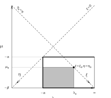
Figure 7: The physically relevant region of the $(\lambda,\mu)$-plane for the determination of the Riemann–Green function $G$, overlayed with the new coordinates $\xi$ and $\eta$ (A.5). The dot marks the source point of the Riemann–Green function $G$ at $(\lambda_{0},\mu_{0})$. This function is non-zero only in the shaded region, which denotes the domain of influence in the $(\lambda,\mu)$-plane of that source point. Fig. 4 on the other hand shows the $(\lambda_{0},\mu_{0})$-plane. It is relevant to the solution for the stress at a single field point $(\lambda,\mu)$. The hatched region $D$ of Fig. 4 shows the domain of dependence of the field point, that is the portion of the source plane on which the solution at the field point depends.

A.2 Laplace transform

We use a Laplace transform to solve (A.4) because the required solution is that to an initial value problem to which Laplace transforms are naturally suited. The PDE is hyperbolic with the lines $\lambda=\mathrm{const}$ and $\mu=\mathrm{const}$ as characteristics, and its solution is non-zero only in the rectangle bounded by the characteristics $\lambda=\lambda_{0}$ and $\mu=\mu_{0}$, and the physical boundaries $\lambda=-\alpha$ and $\mu=-\beta$ (Fig. 7). We introduce new coordinates

$$\xi=(\lambda\!-\!\mu)/\sqrt{2},\qquad\eta=-(\lambda\!+\!\mu)/\sqrt{2},$$ (A.5)

so that eq. (A.4) simplifies to

$$\mathcal{L}^{\star}G\equiv\frac{\partial^{2}G}{\partial\eta^{2}}-\frac{\partial^{2}G}{\partial\xi^{2}}-\frac{\partial}{\partial\xi}\left(\frac{G}{\xi}\right)=2\delta(\xi-\xi_{0})\delta(\eta-\eta_{0}),$$ (A.6)

where $\xi_{0}=(\lambda_{0}\!-\!\mu_{0})/\sqrt{2}$ and $\eta_{0}=-(\lambda_{0}\!+\!\mu_{0})/\sqrt{2}$ are the coordinates of the source point. The factor of 2 arises from the transformation of the derivatives; the product of the delta functions in (A.4) transforms into that of (A.6) because the Jacobian of the transformation (A.5) is unity. The reason for our choice of $\eta$ is that $G\equiv 0$ for $\eta<\eta_{0}$, that is $\lambda+\mu>\lambda_{0}+\mu_{0}$. Hence $\eta$ is a time-like variable which increases in the direction in which the non-zero part of the solution propagates. We take a Laplace transform in $\tilde{\eta}=\eta-\eta_{0}$, and transform $G(\xi,\eta)$ to

$$\hat{G}(\xi,p)=\int\limits_{0}^{\infty}e^{-p\tilde{\eta}}G(\xi,\tilde{\eta}){\mathrm{d}}\tilde{\eta}.$$ (A.7)

There are two equally valid ways of taking proper account of the $\delta(\eta-\eta_{0})$ in taking the Laplace transform of equation (A.6). One can either treat it as $\delta(\tilde{\eta}-0+)$, in which case it has a Laplace transform of 1, or one can treat it as $\delta(\tilde{\eta}-0-)$, in which case it contributes a unit initial value to $\partial G/\partial\eta$ which must be included in the Laplace transform of $\partial^{2}G/\partial\eta^{2}$ (Strauss 1992). Either way leads to a transformed equation for $\hat{G}(\xi,p)$ of

$$p^{2}\hat{G}-\frac{{\mathrm{d}}^{2}\hat{G}}{{\mathrm{d}}\xi^{2}}-\frac{{\mathrm{d}}}{{\mathrm{d}}\xi}\left(\frac{\hat{G}}{\xi}\right)=2\delta(\xi-\xi_{0}).$$ (A.8)

The homogeneous part of eq. (A.8) is the modified Bessel equation of order one in the variable $p\xi$. Two independent solutions are the modified Bessel functions $I_{1}$ and $K_{1}$. The former vanishes at $\xi=0$ and the latter decays exponentially as $\xi\to\infty$. We need $\hat{G}$ to decay exponentially as $\xi\to\infty$ because $G(\xi,\eta)$ vanishes for $\tilde{\eta}<\xi-\xi_{0}$, and hence its Laplace transform $\hat{G}$ is exponentially small for large $\xi$. We also need $\hat{G}$ to vanish at $\xi=0$ where $\lambda=\mu$. The focus at which $\lambda=\mu=-\alpha$ is the only physically relevant point at which $\xi=0$. It lies on a boundary of the solution region in the $\lambda_{0}\to-\alpha$ limit (Fig. 7). The focus is a point at which the difference $\Delta$ between the stresses vanishes, and hence $G$ and $\hat{G}$ should vanish there. The delta function in eq. (A.8) requires that $\hat{G}$ be continuous at $\xi=\xi_{0}$ and that ${\mathrm{d}}\hat{G}/{\mathrm{d}}\xi$ decrease discontinuously by 2 as $\xi$ increases through $\xi=\xi_{0}$. Combining all these requirements, we obtain the result

$$\hat{G}(\xi,p)=\begin{cases}2\xi_{0}\,K_{1}(p\xi)\,I_{1}(p\xi_{0}),&\text{$\xi_{0}\leq\xi<\infty$},\\ 2\xi_{0}\,K_{1}(p\xi_{0})\,I_{1}(p\xi),&\text{$0\leq\xi\leq\xi_{0}$}.\end{cases}$$ (A.9)

We use the Wronskian relation $I_{1}(x)K_{1}^{\prime}(x)-I_{1}^{\prime}(x)K_{1}(x)=-1/x$ (eq. [9.6.15] of Abramowitz & Stegun 1965) in calculating the prefactor of the products of modified Bessel functions. The inversion of this transform is obtained from formula (13.39) of Oberhettinger & Badii (1973) which gives

$$G(\xi,\!\tilde{\eta})\!=\!\!\begin{cases}\!\sqrt{\!\frac{\xi_{0}}{\xi}}\,{}_{2}F_{1}(-\scriptstyle\frac{1}{2}\displaystyle,\scriptstyle\frac{3}{2}\displaystyle;\!1;w),&\text{$|\xi_{0}\!\!-\!\xi|\!\leq\!\tilde{\eta}\!\leq\!\xi_{0}\!\!+\!\xi$},\\ 0,&\text{$-\infty\!<\!\tilde{\eta}\!<\!|\xi_{0}\!\!-\!\xi|$},\end{cases}$$ (A.10)

we have (cf. eq. [3.16])

$$w\equiv\frac{\tilde{\eta}^{2}-(\xi_{0}\!-\!\xi)^{2}}{4\xi_{0}\xi}=\frac{(\lambda_{0}\!-\!\lambda)(\mu_{0}\!-\!\mu)}{(\lambda_{0}\!-\!\mu_{0})(\lambda\!-\!\mu)}.$$ (A.11)

The second case of eq. (A.10) shows that $G$ does indeed vanish outside the shaded sector $\lambda<\lambda_{0}$, $\mu<\mu_{0}$. The first case shows that it agrees with the adjoint Riemann–Green function $\mathcal{G}^{\star}$ of (A.3) which was derived from the analysis of §3.1.

A.3 Comparison with EL89

EL89 use variables $s=-\eta$ and $t=\xi$, whereas we avoided using $t$ for the non-time-like variable. They consider the Fourier transform

$$\bar{G}(\xi,k)=\int\limits_{-\infty}^{\infty}e^{-ik\tilde{\eta}}{G}(\xi,\tilde{\eta}){\mathrm{d}}\tilde{\eta}.$$ (A.12)

Because $G\equiv 0$ for $\tilde{\eta}\leq 0$, we can rewrite our Laplace transform as their Fourier transform. Setting $p=-ik$ gives $\bar{G}(\xi,k)=i\hat{G}(\xi,-ik)$, and using the formulas $I_{1}(x)=-J_{1}(ix)$ and $K_{1}(x)=\frac{1}{2}\pi iH_{1}^{(1)}(ix)$, eq. (A.9) yields

$$\bar{G}(\xi,k)=\begin{cases}\pi i\xi_{0}\,H_{1}^{(1)}(k\xi)\,J_{1}(k\xi_{0}),&\text{$\xi_{0}\leq\xi<\infty$},\\ \pi i\xi_{0}\,H_{1}^{(1)}(k\xi_{0})\,J_{1}(k\xi),&\text{$0\leq\xi\leq\xi_{0}$}.\end{cases}$$ (A.13)

This formula differs from the solution for the Fourier transform given in eq. (70) of EL89. The major difference is that their solution has Hankel functions of the second kind $H_{1}^{(2)}(kt)=H_{1}^{(2)}(k\xi)$ where ours has $J_{1}$ Bessel functions. Consequently their solution has an unphysical singularity at $t=\xi=0$, and so, in our opinion, is incorrect. Our solution, which was devised to avoid that singularity, gives a result which matches that derived by Riemann’s method in §3.1.

A.4 The solution for $\Delta$

The solution for $\Delta$ using the adjoint Riemann–Green function is given by eq. (3.14) with $\mathcal{G}$ replaced by $\mathcal{G}^{\star}$ and the sign of $c_{2}$ changed for the adjoint case (Copson 1975). The hypergeometric function of eq. (A.3) for $\mathcal{G}^{\star}$ is expressible in terms of complete elliptical integrals as

$${}_{2}F_{1}(-\scriptstyle\frac{1}{2}\displaystyle,\scriptstyle\frac{3}{2}\displaystyle;1;w)=\frac{2}{\pi}[E(w)+2wE^{\prime}(w)].$$ (A.14)

Hence, the solution for the difference $\Delta$ between the two principal stresses is given by

$$\Delta(\lambda,\mu)=\frac{2}{\pi(\lambda\!-\!\mu)^{\frac{1}{2}}}\Biggl{\{}\\ \int\limits_{\lambda}^{\infty}{\mathrm{d}}\lambda_{0}\int\limits_{\mu}^{-\alpha}{\mathrm{d}}\mu_{0}\!\Bigl{[}\!E(w)+2wE^{\prime}(w)\!\Bigr{]}\!(\lambda_{0}\!-\!\mu_{0})^{\frac{1}{2}}\!\biggl{(}\!\frac{\partial\rho}{\partial\lambda_{0}}\!\frac{\partial V_{S}}{\partial\mu_{0}}\!-\!\frac{\partial\rho}{\partial\mu_{0}}\!\frac{\partial V_{S}}{\partial\lambda_{0}}\!\biggr{)}\\ -\!\!\int\limits_{\lambda}^{\infty}{\mathrm{d}}\lambda_{0}\!\biggl{[}\!E(w)+2wE^{\prime}(w)\underset{\mu_{0}=-\alpha}{\biggr{]}}\frac{{\mathrm{d}}}{{\mathrm{d}}\lambda_{0}}\!\Bigl{[}\!(\lambda_{0}\!+\!\alpha)^{\frac{1}{2}}\Delta(\lambda_{0},-\alpha)\!\Bigr{]}\!\!\Biggr{\}}.$$ (A.15)

The determined reader can verify, after some manipulation, that this expression is equivalent to the difference between the separate solutions (3.21a) and (3.21b), derived in §3.1.

Note added in manuscript

We agree with the amendment to our method of solution for $\Delta$ given in Appendix A.4. Our Green’s function, while solving the differential equation, had the wrong boundary conditions.
N.W. Evans & D. Lynden-Bell

References

- [1] Abramowitz M., Stegun I. A., 1965, Handbook of Mathematical Functions. New York, Dover Publications
- [2] Arnold R., 1995, MNRAS, 276, 293
- [3] Arnold R., de Zeeuw P. T., Hunter C., 1994, MNRAS, 271, 924
- [4] Bacon R., Simien F., Monnet G., 1983, A&A, 128, 405
- [5] Bak J., Statler T. S., 2000, AJ, 120, 110
- [6] Binney J., 1976, MNRAS, 177, 19
- [7] Binney J., 1978, MNRAS, 183, 501
- [8] Binney J., 1982, MNRAS, 201, 15
- [9] Binney J., Tremaine S., 1987, Galactic Dynamics. Princeton, NJ, Princeton University Press
- [10] Bishop J. L., 1986, ApJ, 305, 14
- [11] Bishop J. L., 1987, ApJ, 322, 618
- [12] Byrd P. F., Friedman M. D., 1971, Handbook of Elliptic Integrals for Engineers and Scientists. Springer-Verlag, Berlin Heidelberg New York, 2nd revised ed.
- [13] Carlson B. C., 1977, Special Functions of Applied Mathematics. Academic Press, New York San Francisco London
- [14] Chandrasekhar S., 1939, ApJ, 90, 1
- [15] Chandrasekhar S., 1940, ApJ, 92, 441
- [16] Conway J., 1973, Functions of one complex variable. New York, Springer-Verlag
- [17] Copson E. T., 1975, Partial Differential Equations. Cambridge, Cambridge University Press
- [18] de Zeeuw P. T., 1985a, MNRAS, 216, 273 [Z85]
- [19] de Zeeuw P. T., 1985b, MNRAS, 216, 599
- [20] de Zeeuw P. T., Hunter C., 1990, ApJ, 356, 365
- [21] de Zeeuw P. T., Hunter C., Schwarzschild M., 1987, ApJ, 317, 607
- [22] de Zeeuw P. T., Peletier R., Franx M., 1986, MNRAS, 221, 1001
- [23] de Zeeuw P. T., Pfenniger D., 1988, MNRAS, 235, 949
- [24] Dejonghe H., de Zeeuw P. T., 1988, ApJ, 333, 90
- [25] Dejonghe H., Laurent D., 1991, MNRAS, 252, 606
- [26] Eddington A. S., 1915, MNRAS, 76, 37
- [27] Evans N., 1990, Intern. J. Computer Math., 34, 105
- [28] Evans N. W., Carollo C. M., de Zeeuw P. T., 2000, MNRAS, 318, 1131
- [29] Evans N. W., de Zeeuw P. T., 1992, MNRAS, 257, 152
- [30] Evans N. W., Lynden-Bell D., 1989, MNRAS, 236, 801 [EL89]
- [31] Evans N. W., Lynden-Bell D., 1991, MNRAS, 251, 213
- [32] Franx M., 1988, MNRAS, 231, 285
- [33] Gebhardt K., Richstone D., Tremaine S., Lauer T. D., Bender R., Bower G., Dressler A., Faber S., Filippenko A. V., Green R., Grillmair C., Ho L. C., Kormendy J., Magorrian J., Pinkney J., 2003, ApJ, in press
- [34] Gerhard O. E., 1993, MNRAS, 265, 213
- [35] Goldstein H., 1980, Classical Mechanics. London, Addison-Wesley
- [36] Hunter C., de Zeeuw P. T., 1992, ApJ, 389, 79 [HZ92]
- [37] Hunter C., de Zeeuw P. T., Park C., Schwarzschild M., 1990, ApJ, 363, 367
- [38] Jeans J. H., 1915, MNRAS, 76, 70
- [39] Kuzmin G., 1973, in Proc. All-Union Conf., Dynamics of Galaxies and Clusters, ed. T.B. Omarov (Alma Ata: Akad. Nauk Kazakhskoj SSR), 71 (English transl. in IAU Symp. 127, Structure and Dynamics of Elliptical Galaxies, ed. P.T. de Zeeuw [Dordrecht: Reidel], 553)
- [40] Lynden-Bell D., 1960, PhD thesis, Cambridge University
- [41] Lynden-Bell D., 1962a, MNRAS, 124, 1
- [42] Lynden-Bell D., 1962b, MNRAS, 124, 95
- [43] Mathieu, A., Dejonghe, H., 1999, MNRAS, 303, 455
- [44] Oberhettinger F., Badii L., 1973, Tables of Laplace Transforms. New York, Springer-Verlag
- [45] Press W. H., Teukolsky S. A., Vettering W. T., Flannery B. P., 1992, Numerical Recipes. Cambridge Univ. Press, Cambridge
- [46] Qian E. E., de Zeeuw P. T., van der Marel R. P., Hunter C., 1995, MNRAS, 274, 602
- [47] Rix H., de Zeeuw P. T., Cretton N., van der Marel R. P., Carollo C. M., 1997, ApJ, 488, 702
- [48] Robijn F. H. A., de Zeeuw P. T., 1996, MNRAS, 279, 673
- [49] Schwarzschild M., 1979, ApJ, 232, 236
- [50] Schwarzschild M., 1993, ApJ, 409, 563
- [51] Stäckel P., 1890, Math. Ann., 35, 91
- [52] Stäckel P., 1891, Über die Integration der Hamilton-Jacobischen Differential gleichung mittelst Separation der Variabeln. Habilitationsschrift, Halle
- [53] Statler T. S., 1987, ApJ, 321, 113
- [54] Statler T. S., 1991, AJ, 102, 882
- [55] Statler T. S., 1994a, ApJ, 425, 458
- [56] Statler T. S., 1994b, ApJ, 425, 500
- [57] Statler T. S., 2001, AJ, 121, 244
- [58] Statler T. S., Fry A. M., 1994, ApJ, 425, 481
- [59] Statler, T. S., Dejonghe, H., Smecker-Hane, T., 1999, AJ, 117, 126
- [60] Strauss W. A., 1992, Partial Differential Equations. New York, John Wiley
- [61] van der Marel R. P., Cretton N., de Zeeuw P. T., Rix H., 1998, ApJ, 493, 613
- [62] Verolme E. K., Cappellari M., Copin Y., van der Marel R. P., Bacon R., Bureau M., Davies R., Miller B., de Zeeuw P. T., 2002, MNRAS, 335, 517
- [63] Weinacht J., 1924, Math. Ann., 91, 279
- [64] Zhao H. S., 1996, MNRAS, 283, 149