Large Angle CMB Fluctuations from Cosmic Strings with a Comological Constant

Abstract

In this paper, we present results for large-angle CMB anisotropies generated from high resolution simulations of cosmic string networks in a range of flat FRW universes with a cosmological constant. Using an ensemble of all-sky maps, we compare with the COBE data to infer a normalization (or upper bound) on the string linear energy density $\mu$. For a flat matter-dominated model ($\Omega_{M}=1$) we find $G\mu/c^{2}\approx 0.7\times 10^{-6}$, which is lower than previous constraints probably because of the more accurate inclusion of string small-scale structure. For a cosmological constant within an observationally acceptable range, we find a relatively weak dependence with $G\mu/c^{2}$ less than 10% higher.

I Introduction

Given the growing evidence for a cosmological constant or dark energy component in the Universe, it is important to determine whether this significantly impacts the evolution of cosmic strings and their observational signatures. The strongest constraints limiting the energy scale of cosmic strings is currently the COBE normalisation of large-angle CMB anisotropy. In this paper, we will infer this normalisation from maps computed using the methods presented in Landriau and Shellard (2003) and determine how this is influenced by late-time domination by a cosmological constant.

II Method

II.1 Geometry of Simulations

To compute all-sky maps, the “observers” are located inside the simulation box. Following Pen et al. (1994), we place eight such observers at each corner of a cube of side $L/2$ where $L$ is the size of the box itself. We use the fact that the string networks, and hence the cosmological perturbations they induce, have periodic boundary conditions to identify opposite sides of the box. The eight realizations of the sky are not completely independent, but the correlations are not apparent. This scheme reduces the effect of the cosmic variance on large angular scales and thus renders the computation of the normalization more accurate.

II.2 Pixelization

To facilitate the computation of maps and the extraction of the power spectrum, we use an iso-latitude pixelization, which enables us to Fourier transform each ring of constant $\theta$ to evaluate the integral over the azimuthal angle. More specifically, we use the equal area with 3:6:3 base pixels, proposed by Crittenden and Turok (1998). In this scheme, each base pixel is subdivided into $n^{2}=2^{2p}$ pixels. The area of a pixel is given by $A_{pixel}=4\pi/N_{pixel}=\pi/3n^{2}$. But, by integrating the spherical surface element over a pixel, we have $A_{pixel}=\frac{2\pi}{N_{p}}\Delta\cos\theta$. Hence, the width of a row of pixels is given by

$$\Delta\cos\theta=\frac{N_{p}}{6n^{2}}\,,$$ (1)

where $N_{p}$ is the number of pixels per row of constant $\theta$. In the polar caps, $N_{p}=3$, then $9\times 2^{i-2}$ repeated $2^{i-2}$ times with $2\leq i\leq p+2$. The equatorial regions are made up of $n$ rows of $6n$ pixels.

II.3 Angular Power Spectrum Computations

The pixelized map is the convolution of the real temperature map with the pixel window function. To compute the power spectrum, we need to know the spherical transform of the window function. In real space, the pixel window function is simply given by:

$$W^{pq}(\phi,\theta)=\left\{\begin{array}[]{ll}\frac{1}{A_{pixel}}&\mbox{inside the pixel}\\ 0&\mbox{outside}\end{array}\right.\,,$$ (2)

where $p$ and $q$ label the rows and the pixels on that row:

$$\begin{array}[]{ll}T^{pq}&=\displaystyle\int_{\mathcal{S}_{2}}T(\phi,\theta)W^{pq}(\phi,\theta)d\Omega\\ &=\displaystyle\sum_{m=-\ell_{max}}^{\ell_{max}}b_{m}e^{\dot{\imath}mq2\pi/N_{p}}\,,\end{array}$$ (3)

where

$$b_{m}=\displaystyle\sum_{\ell=|m|}^{\ell_{max}}a_{\ell m}w(\pi m/N_{p})\overline{\lambda_{\ell}^{m}}\,,$$ (4)

with

$$\begin{array}[]{c}w(\psi)=e^{\dot{\imath}\psi}\frac{\sin\psi}{\psi}\\ \overline{\lambda_{\ell}^{m}}=\frac{1}{\cos\theta_{p}-\cos\theta_{p+1}}\int_{\cos\theta_{p}}^{\cos\theta_{p+1}}\lambda_{\ell}^{m}(\cos\theta)d(\cos\theta)\,,\end{array}$$ (5)

From the last line in (3), the $b_{m}$ can be obtained by the inverse sum:

$$b_{m}=\sum_{q}T_{pq}e^{-\dot{\imath}mq2\pi/N_{p}}\,,$$ (6)

which can be done using a Fast Fourier Transform. The sum (4) can also be inverted to obtain the $a_{\ell m}$’s:

$$a_{\ell m}=\frac{\sum_{p=1}^{n_{rows}}b_{m}w^{*}(\pi m/N_{p})\overline{\lambda_{\ell}^{m}}}{\sum_{p=1}^{n_{rows}}w^{*}(\pi m/N_{p})w(\pi m/N_{p})N_{p}}\,.$$ (7)

To obtain this last equation, we took the approximation that the pixelized spherical harmonics $w(\pi m/N_{p})\overline{\lambda_{\ell}^{m}}$ are orthogonal, which is valid at low $\ell$.

II.4 COBE Normalisation

To infer the cosmic string linear energy density, we use the COBE angular correlation function because, on the scales of interests, it is good as that of WMAP Halpern (2003). This also enables direct comparisons with previous work.

To normalize to COBE, we follow Allen et al. (1996) and compute the angular correlation function using

$$C(\theta,\theta_{s})=\frac{1}{4\pi}\sum_{\ell}(2\ell+1)|W_{\ell}|^{2}|B_{\ell}|^{2}C_{\ell}P_{\ell}(\cos\theta)\,,$$ (8)

where we use the following smoothing function:

$$W_{\ell}(\theta)=\exp\left(-\frac{\ell(\ell+1)}{\log 2}\sin^{2}(\theta/4)\right)\,,$$ (9)

where $\theta$ is the smoothing scales. We also use the COBE beam profile $B_{\ell}$ given in Wright et al. (1994).We then compare the result with the value obtained by the four year COBE maps Banday et al. (1997), $C(0^{\circ},10^{\circ})=(29\pm 1\mu K/T)^{2}$ to infer the value of $G\mu/c^{2}$. In the previous equation, $T$ is the mean temperature of the CMB also obtained from COBE Bennett et al. (1996) $T=2.726\pm 0.002K$.

III Results

III.1 Cosmic String Simulations

We created a time series of cosmic string realizations using the Allen-Shellard network simulation Allen and Shellard (1990) in a variety of flat FRW universes with $\Omega_{m}+\Omega_{\Lambda}=1$, where $\Omega_{m}$ includes the contribution of dark matter and baryons. These string networks were then used as sources for the CMB map-making pipeline. For all the simulations, we chose $h=0.72$ and $\Omega_{b}h^{2}=0.02$.

Two string simulations for $\Omega_{\Lambda}=0$ and $\Omega_{\Lambda}=0.7$ were computed with very high resolution with over 3 million points (16 ponts per correlation length) and spanning a dynamic range of 5 in conformal time, probing the Universe back to $z=25$ and $z=30$ respectively. All string loops were retained in the simulation to ensure overall network energy-momentum conservation, which was preserved at the level of 1%. Point-joining was used only to ensure a consistent physical resolution, i.e. removing very short segments formed through reconnection. The simulations therefore retained their full small-scale structure. These were the costliest part of the pipeline and took many days to perform on the COSMOS supercomputer (approximately 2000 hours of CPU time). This improves upon previous work with string networks in an expanding Universe, which was performed with fewer points per correlation length, fixed horizon resolution and a separate treatment of loops Allen et al. (1996, 1997).

In addition, we performed a series of smaller simulations (1 million points) for different values of the cosmological constants, specifically, $\Omega_{\Lambda}=0,\,0.2,\,0.4,\,0.55,\,0.7,\,0.85$. These simulations had identical initial conditions, so comparisons could minimize the effects of cosmic variance.

The map-making pipeline was tested at resolutions of $128^{3}$ and $256^{3}$. The huge data storage requirements with string networks, SVT-decomposed energy-momentum tensor grids, Boltzmann code output plus checkpointing files meant disk space approaching 1Tbyte was required for $256^{3}$. Further parallelisation issues remain to be resolved for large memory runs.

In figure 1, we present realizations for the $\Omega_{\Lambda}=0$ and $0.7$ runs.

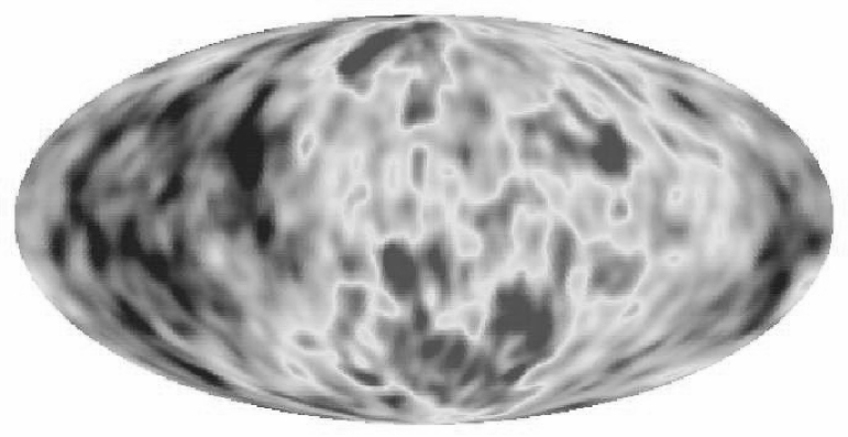
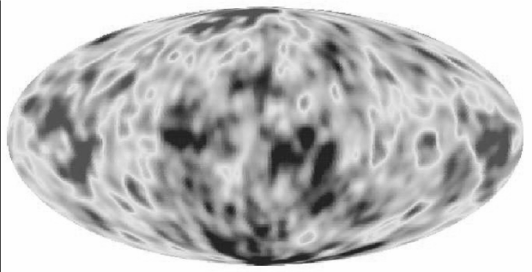
Figure 1: All-sky string-induced maps for a flat FRW Universe with $\Omega_{\Lambda}=0$ and. $0.7$

The angular power spectra for each of these runs are presented in figure 3. We also show four spectra obtained from the $\Omega_{\Lambda}=0$ run with their average in figure 2. All these spectra are normalised to COBE.

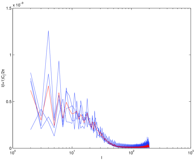
Figure 2: Individual power spectra for the $\Omega_{\Lambda}=0$ run in blue with the average in red.

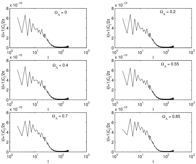
Figure 3: Average power spectra for each run.

III.2 Normalization to COBE

The power spectra illustrated in figures 2 and 3 show a roughly scale invariant plateau for $\ell\mathrel{\hbox to0.0pt{\lower 4.0pt\hbox{\hskip 1.0pt$\sim$}\hss}\raise 1.0pt\hbox{$<$}}20$ with a gradual fall-off to an insignificant signal beyond $\ell\mathrel{\hbox to0.0pt{\lower 4.0pt\hbox{\hskip 1.0pt$\sim$}\hss}\raise 1.0pt\hbox{$>$}}50$. This fall-off is a consequence of the limited dynamic range of the string simulations and not of the resolution at which the Boltzmann evolution was performed (though there is some influence from the interpolation and smoothing of the string network onto the grids.

Previous CMB work with string networks over a much larger dynamic range has demonstrated that the main anisotropies relevant to COBE are generated at redshifts $z\mathrel{\hbox to0.0pt{\lower 4.0pt\hbox{\hskip 1.0pt$\sim$}\hss}\raise 1.0pt\hbox{$<$}}20$ Allen et al. (1996), which is within the range of the present work. The reason for this can be seen from studies of the unequal-time correlators (UETC’s) Albrecht et al. (1996); Wu et al. (2002), which peak on scales well below the horizon $(\lambda_{max}<d_{H}/3$). We are confident therefore that our simulations include the primary contributions on COBE scales.

This scale invariance on large angular scales is consistent with the COBE data and allows us to normalize our results accordingly, as discussed above, providing a constraint on the energy density of strings. Our normalization for the flat CDM model,

$$\frac{G\mu}{c^{2}}=(0.7\pm 0.2)\times 10^{-6}\,,$$ (10)

has an error reflecting the variance of our results, not systematic effects which may be comparable. This result is lower but consistent with the previous result Allen et al. (1996):

$$\frac{G\mu}{c^{2}}=(1.05^{+0.35}_{-0.2})\times 10^{-6}\,.$$ (11)

Our result is significantly lower than the one obtained in Allen et al. (1997), $G\mu/c^{2}=1.7\times 10^{-6}$ from a single simulation. This work however focused on small angle anisotropies and did not study sample variance at large angles. Other flat space approximations and semi-analytic estimates for local string networks generally have found a higher normalization than ours, e.g. $G\mu/c^{2}=(1.5\pm 0.5)\times 10^{-6}$ Bennett et al. (1992), $G\mu/c^{2}=(1.7\pm 0.7)\times 10^{-6}$ Perivolaropoulos (1993) and $G\mu/c^{2}=2$ Coulson et al. (1994).

However, there is a key reason why the present work is a significant advance over these previous analyses. Apart from now including all the relevant physics, this analysis uses the highest resolution string simulations to date. The initial points per correlation length have been chosen at levels known to preserve small scale structure accurately Martins and Shellard (2001) and the simulations are evolved at fixed physical resolution. Although the simulations used in Allen et al. (1996) spanned a larger dynamic range, $z<100$ (compared to our $z<25$), it did so by maintaining fixed horizon resolution through point-joining and smoothing. Subsequent work has shown that at least comoving resolution is required if we are to hope for a satisfactory treatment of string wiggliness. This implies that the previous work did not adequately account for the renormalized string energy per unit length, which in the matter era is $\tilde{\mu}\simeq 1.4\mu$. Such a factor would tend to increase the string anisotropy, thus lowering the COBE normalization of $G\mu/c^{2}$ (though in a non-trivial manner).

III.3 Effect of the Cosmological Constant

The influence of $\Omega_{\Lambda}$ on the COBE normalization, illustrated in figure 5 is relatively small: for the popular value of $\Omega_{\Lambda}=0.7$ we obtained $G\mu/c^{2}=(0.74\pm 0.20)\times 10^{-6}$, only 6% higher than for the flat CDM model.

The reason for the reduced anisotropy in $\Lambda$-models is fairly clear. As the Universe becomes vacuum dominated at late times, the expansion rate increases, affecting the Hubble damping term $\dot{a}/a$ in the string equations of motion, thus lowering their average velocity as can be seen from figure 4.

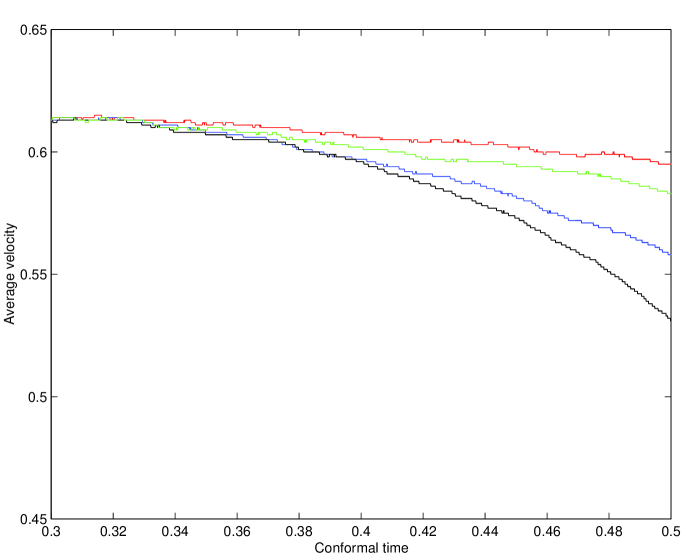
Figure 4: Average rms long string velocity for the last half of the string network simulations for $\Omega_{\Lambda}=0$ (red), $\Omega_{\Lambda}=0.4$ (green), $\Omega_{\Lambda}=0.7$ (blue) and $\Omega_{\Lambda}=0.85$ (black). Even the extremal $\Lambda$-model shows only a relatively small 11% decline in the average string velocity by the present day. (Relative conformal time is plotted with $\eta_{0}=0.5$.)

As string velocities are the primary cause of CMB anisotropies, there will be a net reduction in $\Delta T/T$.

The smallness of this effect is somewhat surprising, but is explained by the late redshift of vacuum domination. In the $\Omega_{\Lambda}=0.7$, this occurs at $z_{\Lambda}\simeq 0.33$, which, in the context of our simulations, implies that $\Lambda$ has a significant effect on only the later stages of the simulation. Comparing the $\Omega_{\Lambda}=0.85$ model with the flat CDM model in figure 3, there appears to be a slight relative fall-off in the average power towards $\ell=2$, which is consistent with this picture. However, this effect is likely to be swamped by cosmic variance.

We have found that our data points are well fitted by

$$\frac{G\mu}{c^{2}}=\left(0.695+\frac{0.012}{1-\Omega_{\Lambda}}\right)\times 10^{-6}\,.$$ (12)

This analytic fit is motivated by the asymptotic limit in which string velocities should vanish as the network is frozen and conformally streched in an extreme $\Lambda$-model: $\Omega_{\Lambda}\rightarrow 1$ and $\Omega_{m}\rightarrow 0$. Our results are summarized in table 1 and plotted in figure 5 along with the fit (12).

$\Omega_{\Lambda}$	$G\mu/c^{2}\times 10^{-6}$
0.00	0.7038 $\pm$ 0.1947
0.20	0.7170 $\pm$ 0.1926
0.40	0.7133 $\pm$ 0.1989
0.55	0.7189 $\pm$ 0.1902
0.70	0.7389 $\pm$ 0.1990
0.85	0.7766 $\pm$ 0.1879

Table 1: String linear energy density obtained from the COBE normalisation.

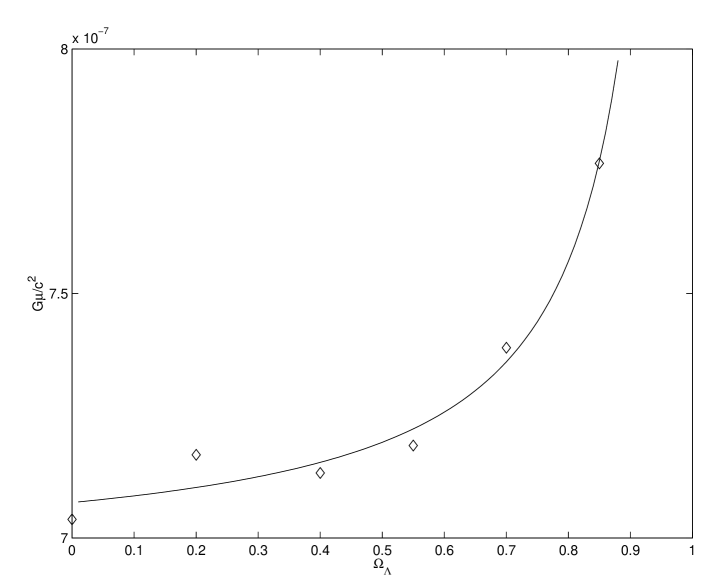
Figure 5: String linear energy density obtained from the COBE normalisation. The solid line is the curve (12).

IV Summary

In this paper, we presented large angle maps of CMB fluctuations seeded by networks of cosmic strings in flat FRW universes with a cosmological constant. From the COBE data, we have obtained a constraint on the string linear energy density $G\mu/c^{2}\mathrel{\hbox to0.0pt{\lower 4.0pt\hbox{\hskip 1.0pt$\sim$}\hss}\raise 1.0pt\hbox{$<$}}0.7\times 10^{-6}$ which is lower than previous work because string small-scale structure is incorporated more accurately in the network simulations. We were able to find the dependence of the string density $\mu$ as a function of the cosmological constant, obtaining a good fit with a simple semi-analytic formula. Given the uncertainties in the overall normalization, these results should provide an adequate means by which to characterise the effects of $\Omega_{\Lambda}$ on cosmic string models.

Although current CMB data have shown that cosmic strings cannot be the dominating source of CMB anisotropies (e.g. Bennett et al. (2003)), they can nonetheless be present albeit at a lower energy scale. For example, they are copiously produced at the end of brane inflation Sarangi and Tye (2002); Pogosian et al. (2003). With this in mind, our normalisation appears low when compared with the value inferred from the possible detection of a gravitational lensing event by a cosmic string: $G\mu/c^{2}\approx 0.4\times 10^{-6}$ Sazhin et al. (2003). This linear mass density would be somewhat higher than allowed in the standard cosmic string scenario considered in this paper.

References

- Landriau and Shellard (2003) M. Landriau and E. P. S. Shellard, Physical Review D67, 103512 (2003).
- Pen et al. (1994) U. L. Pen, D. N. Spergel, and N. Turok, Phys.Rev. D49, 692 (1994).
- Crittenden and Turok (1998) R. G. Crittenden and N. G. Turok (1998), astro-ph/9806374.
- Halpern (2003) M. Halpern (2003), private communication.
- Allen et al. (1996) B. Allen, R. R. Caldwell, E. P. S. Shellard, A. Stebbins, and S. Veeraraghavan, Phys.Rev.Lett. 77, 3061 (1996).
- Wright et al. (1994) E. L. Wright et al., ApJ 420, 1 (1994).
- Banday et al. (1997) A. J. Banday et al., ApJ 475, 393 (1997).
- Bennett et al. (1996) C. L. Bennett et al., ApJ Letters 464, L1 (1996).
- Allen and Shellard (1990) B. Allen and E. P. S. Shellard, Phys.Rev.Lett. 64, 119 (1990).
- Allen et al. (1997) B. Allen, R. R. Caldwell, S. Dodelson, L. Knox, E. P. S. Shellard, and A. Stebbins, Phys.Rev.Lett. 79, 2624 (1997).
- Albrecht et al. (1996) A. Albrecht, D. Coulson, P. G. Ferreira, and J. Magueijo, Phys.Rev.Lett. 76, 1413 (1996).
- Wu et al. (2002) J. H. P. Wu, P. P. Avelino, E. P. S. Shellard, and B. Allen, Int.J.Mod.Phys. D11, 61 (2002).
- Bennett et al. (1992) D. P. Bennett, A. Stebbins, and F. R. Bouchet, ApJ Letters 399, L5 (1992).
- Perivolaropoulos (1993) L. Perivolaropoulos, Phys.Lett. B298, 305 (1993).
- Coulson et al. (1994) D. Coulson, P. Ferreira, P. Graham, and N. Turok, Nature 368, 27 (1994).
- Martins and Shellard (2001) C. J. A. P. Martins and E. P. S. Shellard (2001), unpublished.
- Bennett et al. (2003) C. L. Bennett et al., ApJS 148, 1 (2003).
- Sarangi and Tye (2002) S. Sarangi and S. H. H. Tye, Phys. Lett. B536, 185 (2002).
- Pogosian et al. (2003) L. Pogosian, S. H. H. Tye, I. Wasserman, and M. Wyman, Phys. Rev. D68, 023506 (2003).
- Sazhin et al. (2003) M. Sazhin et al. (2003), astro-ph/0302547.