Fireballs, Flares and Flickering

Abstract

We review our understanding of the prototype “Propeller” system AE Aqr and we examine its flaring behaviour in detail. The flares are thought to arise from collisions between high density regions in the material expelled from the system after interaction with the rapidly rotating magnetosphere of the white dwarf. We show calculations of the time-dependent emergent optical spectra from the resulting hot, expanding ball of gas and derive values for the mass, lengthscale and temperature of the material involved. We see that the fits suggest that the secondary star in this system has reduced metal abundances and that, counter-intuitively, the evolution of the fireballs is best modelled as isothermal.

Louisiana State University, Department of Physics and Astronomy, Nicholson Hall, Baton Rouge, LA 70803-4001, U.S.A.

School of Physics and Astronomy, University of St. Andrews, North Haugh, St. Andrews, Fife, KY16 9SS, U.K.

Department of Physics and Astronomy, University of California, Irvine, 4129 Frederick Reines Hall, Irvine, CA 92697-4574, U.S.A.

1. Introduction

AE Aqr is a long period CV ($P_{\rm orb}=9.88~{}{\rm h}$), implying that the secondary is somewhat evolved. Coherent oscillations in optical (Patterson 1979), ultraviolet (Eracleous et al. 1994), and X-ray (Patterson et al. 1980) lightcurves reveal the white dwarf’s 33s spin period. The oscillation has two unequal peaks per spin cycle, consistent with broad hotspots on opposite sides of the white dwarf $\sim 15^{\circ}$ above and below the equator (Eracleous et al. 1994). These oscillations are strongest in the ultraviolet, where their spectra show a blue continuum with broad Ly $\alpha$ absorption consistent with a white dwarf ($\log{g}\approx 8$) atmosphere with $T\sim 3\times 10^{4}~{}{\rm K}$ (Eracleous et al. 1994). The simplest interpretation is accretion heating near the poles of a magnetic dipole field tipped almost perpendicular to the rotation axis.

An 11-year study of the optical oscillation period (de Jager et al. 1994) showed that the white dwarf is spinning down at an alarming rate. Something extracts rotational energy from the white dwarf at a rate $I\omega\dot{\omega}\sim 60\nu L_{\nu}$ ie. some 60 times the luminosity of the system. We now believe that to be a magnetic propeller. This model was first proposed by Wynn, King, & Horne (1995) and Eracleous & Horne (1996) and expanded upon in Wynn, King & Horne (1997) with comparison of observed and modelled tomograms. Further work on the flaring region was reported in Welsh, Horne & Gomer (1998) and Horne (1999).

The gas stream emerging from the companion star through the L1 nozzle encounters a rapidly spinning magnetosphere. The rapid spin makes the effective ram pressure so high that only a low-density fringe of material becomes threaded onto field lines. Most of the stream material remains diamagnetic, and is dragged toward co-rotation with the magnetosphere. As this occurs outside the co-rotation radius, this magnetic drag propels material forward, boosting its velocity up to and beyond escape velocity. The material emerges from the magnetosphere and sails out of the binary system. This process efficiently extracts energy and angular momentum from the white dwarf, transferring it via the long-range magnetic field to the stream material, which is expelled from the system. The ejected outflow consists of a broad equatorial fan of material launched over a range of azimuths on the side away from the secondary..

The material stripped from the gas stream and threaded by the field lines has a different fate, one which we believe gives rise to the radio and X-ray emission. This material co-rotates with the magnetosphere while accelerating along field lines either toward or away from the white dwarf under the influences of gravity and centrifugal forces. The small fraction of the total mass transfer that leaks below the co-rotation radius at $\sim 5~{}R_{\rm wd}$ accretes down field lines producing the surface hotspots responsible for the 33s oscillations. Particles outside co-rotation remain trapped long enough to accelerate up to relativistic energies through magnetic pumping, eventually reaching a sufficient energy density to break away from the magnetosphere (Kuijpers et al. 1997). The resulting ejection of balls of relativistic magnetized plasma is thought to give rise to the flaring radio emission (Bastian, Dulk & Chanmugam 1998a,b).

In many studies the lightcurves exhibit dramatic flares, with 1-10 minute rise and fall times (Patterson 1979; van Paradijs, Kraakman & van Amerongen 1989; Bruch 1991; Welsh, Horne & Oke 1993). The flares seem to come in clusters or avalanches of many super-imposed individual flares separated by quiet intervals of gradually declining line and continuum emission (Eracleous & Horne 1996; Patterson 1979). These quiet and flaring states typically last a few hours. Power spectra computed from the lightcurves have a power-law form, with larger amplitudes on longer timescales. Similar red noise power spectra are seen in active galaxies, X-ray binaries, and other cataclysmic variables, and is therefore regarded as characteristic of accreting sources in general. However, flickering in other cataclysmic variables typically has an amplitude of 5-20% (Bruch 1992), contrasting with factors of several in AE Aqr. If the mechanism is the same, then it must be weaker or dramatically diluted in other systems. The extreme behaviour in AE Aqr may thus allow us to probe the underlying physics involved where the resultant effects are clearest.

The optical and ultraviolet spectra of the AE Aqr flares are not understood at present except in the most general terms. The lines and continua rise and fall together, with little change in the equivalent widths or ratios of the emission lines (Eracleous & Horne 1996). This suggests that the flares represent changes in the amount of material involved more than changes in physical conditions. Ultraviolet spectra from HST reveal a wide range of lines representing a diverse mix of ionization states and densities. Eracleous & Horne (1996) concluded that a large fraction of the line-emitting gas the density is in the range $n\sim 10^{15}$–$10^{17}~{}{\rm m}^{-3}$ and that denser regions likely also exist. The CIV emission is unusually weak, suggesting non-solar abundances consistent with the idea that the secondary is evolved. Latest results of ultraviolet observations and abundance analysis of the secondary are presented by Mouchet (this volume) and Bonnet-Bidaud (this volume).

What mechanism triggers these dramatic optical and ultraviolet flares? Clues come from multi-wavelength co-variability and orbital kinematics. Simultaneous VLA and optical observations show that the radio flux variations occur on similar timescales but are not correlated with the optical and ultraviolet flares, which therefore require a different mechanism (Abada-Simon et al. 1995). It has been proposed that the flares represent modulations of the accretion rate onto the white dwarf, so that they should be correlated with X-ray variability. Some correlation was found, but the correlation is not high. However, HST observations discard this model, because the ultraviolet oscillation amplitude is unmoved by transitions between the quiet and flaring states (Eracleous & Horne 1996). This disconnects the origins of the oscillations and flares, and the oscillations arise from accretion onto the white dwarf, so the flares must arise elsewhere.

Further clues come from emission line kinematics. The emission line profiles may be roughly described as broad Gaussians with widths $\sim 1000$ km s^-1, though they often exhibit kinks and sometimes multiple peaks. Detailed study of the Balmer lines (Welsh et al. 1998) indicates that the new light appearing during a flare can have emission lines shifted from the line centroid and somewhat narrower, $\sim 300$ km s^-1. Individual flares therefore occupy only a subset of the entire emission-line region.

The emission line centroid velocities vary sinusoidally with orbital phase, with semi-amplitudes $\sim 200$ km s^-1 and maximum redshift near phase $\sim$0.8 (Welsh et al. 1998). These unusual orbital kinematics are shared by both ultraviolet and optical emission lines. The implication is that the flares arise from gas moving with a $\sim 200$ km s^-1 velocity vector that rotates with the binary and points away the observer at phase 0.8. This is hard to understand in the standard model of a cataclysmic variable star, though many (eg. SW Sex systems) show similar anomalous emission-line kinematics (Thorstensen et al. 1991) suggesting a common underlying mechanism. In particular, Kepler velocities in an AE Aqr accretion disc would be $>600$ km s^-1 (though we believe no disc to be present.) The gas stream has a similar direction but its velocity is $\sim 1000$ km s^-1. A success of the magnetic propeller model is its ability to account for the anomalous emission-line kinematics. The correct velocity amplitude and direction occurs in the exit fan just outside the Roche lobe of the white dwarf. But the question remains of why the flares are ignited here, several hours after the gas slips silently through the magnetosphere.

The key insight which solved this puzzle was the realization that the magnetic propeller acts as a blob sorter. More compact, denser, diamagnetic blobs are less affected by magnetic drag. They punch deeper into the magnetosphere and emerge at a larger azimuth with a smaller terminal velocity. These compact blobs can therefore be overtaken by ‘fluffier’ blobs ejected with a larger terminal velocity in the same direction, having left the companion star somewhat later but having spent less time in the magnetosphere (Wynn et al. 1997). The result is a collision between two gas blobs, which can give rise to shocks and flares. Calculations of the trajectories of magnetically propelled diamagnetic blobs with different drag coefficients indicate that they cross in an arc-shaped region of the exit stream, in just the right place to account for the orbital kinematics of the emission lines (Welsh et al. 1998; Horne 1999). Figure 1 shows how these trajectories map to a locus of points in the lower left quadrant of the Doppler map that is otherwise difficult to populate.

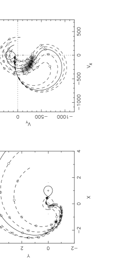
Figure 1.: Trajectories of diamagnetic blobs passing though the AE Aquarii system with the corresponding Doppler tomogram. The open circles mark the time of flight in units of $0.1~{}P_{\rm orb}$. Asterisks and grey patches mark the locations where lower density blobs overtake and collide with more compact blobs, producing fireballs. This occurs in the lower left quadrant at the location corresponding to the observed emission lines.

There remains the problem of developing a quantitative understanding of the unusual emission-line spectra resulting from the collision.

2. Fireball Models

2.1. Typical Parameters

We can derive rough estimates for the physical parameters associated with the colliding blobs by using the typical rise time $t\sim 300~{}{\rm s}$ and an observed optical flux $f_{\nu}\sim 50$ mJy with a closing velocity $V\sim 300~{}{\rm km~{}s}^{-1}$ for the blobs, together with a distance of 100pc. A summary of typical values is provided in Table 1.

Quantity	Value
observed flux $f_{\nu}$	$50$	mJy
closing velocity $V$	$300$	$\rm{km~{}s}^{-1}$
flare risetime $t_{\rm rise}$	300	s
mass transfer rate $\dot{M}$	$10^{14}$	${\rm kg~{}s}^{-1}$
fireball mass $M$	$3\times 10^{16}$	kg
pre-collision lengthscale $a$	$9\times 10^{7}$	m
initial temperature $T$	$10^{6}$	K
total energy $E$	$3\times 10^{26}$	J
typical density $\rho$	$3\times 10^{-8}$	${\rm kg~{}m}^{-3}$
number density $n$	$3\times 10^{19}$	${\rm m}^{-3}$
column density $N$	$3\times 10^{27}$	${\rm m}^{-2}$

Table 1.: Estimates of typical values for flare quantities.

2.2. Expansion

We envision an expanding fireball emerging from the aftermath of a collision between two masses $m_{1}+m_{2}=M$. With nothing to hold it back, the hot ball of gas expands at the initial sound speed, launching a fireball. We adopt a uniform, spherically symmetric, Hubble-like expansion $V=Hr_{0}=Hr/\beta$, in which the Eulerian radial coordinate $r$ of a gas element is given in terms of its initial position $r_{0}$ and time $t$ by

$$r(r_{0},t)=r_{0}+v(r_{0})t=r_{0}+Hr_{0}t=r_{0}(1+Ht)\equiv r_{0}\beta.$$ (1)

This defines an expansion factor $\beta$ which we can use as a dimensionless time parameter. The ‘Hubble’ constant is set by the initial conditions $Ha_{\rm i}\approx v(a_{\rm i})\approx c_{\rm s,i}$. If we can determine parameters at some time $t=0$ ie. $\beta=1$ for the lengthscale ($a_{0}$), temperature ($T_{0}$) and mass ($M$), we can derive the time evolution as follows. We adopt a Gaussian density profile

$$\rho(r,t)=\rho_{0}\beta^{-3}e^{-\eta^{2}}$$ (2)

where $\rho_{0}$ is the central density at $t=0$ and $\eta\equiv\frac{r_{0}}{a_{0}}=\frac{r}{a}$ is a dimensionless radius coordinate: the radius $r$ scaled to the lengthscale $a=\beta a_{0}$. This Gaussian density is motivated by the Gaussian shapes of observed, Doppler-broadened, line profiles.

2.3. Cooling

We consider two cooling schemes: adiabatic and isothermal. The adiabatic fireball cools purely as a result of its expansion and corresponds to a situation where the radiative and recombination cooling rates are negligible. In contrast, the isothermal model maintains a fixed temperature throughout its evolution. A truly isothermal fireball would require a finely balanced energy source to counteract the expansion cooling. However, it may be an appropriate approximation to a situation where a photospheric region dominates the emission and presents a fixed effective temperature to the observer as a result of the stong dependence of opacity on temperature. For adiabatic expansion we can show that an initially uniform temperature distribution remains uniform and so,

$$T(r,t)=T_{0}\beta^{-3(\gamma-1)}.$$ (3)

With $\gamma=5/3$ for a monatomic gas, $T\propto\beta^{-2}$, and so the sound speed $c_{\rm s}\propto T^{1/2}\propto\beta^{-1}$. The sound crossing time $a/c_{\rm s}\propto\beta^{2}$. and so the fireball becomes almost immediately supersonic.

2.4. Ionization Structure

In the LTE approximation, the density and temperature determine the ionization state of the gas at each point in space and time through the solution of a network of Saha equations. Atomic level populations are similarly determined through Boltzmann factors and partition functions.

Once we have determined the evolution of $T$ and $\rho$ with time, we can follow the evolution of the ionization structure. At a given time, the various ionic species form onion layers of increasing ionization on moving outwards from the fireball centre. The adiabatic temperature evolution causes the ionization states to alter rapidly throughout the structures when the fireball passes the appropriate critical temperatures. Isothermal evolutions show the gentler dependance of ionization on density. The spatial structure remains roughly constant and only evolves slowly as the density drops.

3. Radiative Transfer

The radiative transfer equation has a formal solution

$$I=\int Se^{-\tau}d\tau,$$ (4)

where $I$ is the intensity of the emerging radiation, $S$ is the source function, and $\tau$ is the optical depth measured along the line of sight from the observer. This integral sums contributions $Sd\tau$ to the radiation intensity, attenuating each by the factor $e^{-\tau}$ because it has to pass through optical depth $\tau$ to reach the observer.

Since we have assumed LTE, the source function is the Planck function, and opacities both for lines and continuum are also known once the velocity, temperature, and density profiles and element abundances are specified. The integral can therefore be evaluated numerically, either in this form or more quickly by using Sobolev resonant surface approximations.

The above line integral gives the intensity $I(y)$ for lines of sight with different impact parameters $y$. We let $x$ measure distance from the fireball centre toward the observer, and $y$ the distance perpendicular to the line of sight. The fireball flux, obtained by summing intensities weighted by the solid angles of annuli on the sky, is then

$$f(\lambda)=\int_{0}^{\infty}I(\lambda,y)\frac{2\pi y}{d^{2}}dy$$ (5)

where $d$ is the source distance.

4. Comparison with Observations

4.1. Observed Flare in AE Aqr

To test the fireball models, we compared them to high time-resolution optical spectra of an AE Aqr flare taken with the Keck telescope (Skidmore et al. 2003). The lightcurve formed from these data is plotted in Fig. 2. Although the dataset only lasts around 13 minutes it shows the end of one flare and beginning of another. The major features of the flaring observed in the system are apparent in the lightcurve.

Figure 2.: Observed lightcurve reported in Skidmore et al. (2003) showing the decline of an old flare and start of a small new flare.

We extracted the spectrum of the second flare by subtracting the quiescent spectrum (Q) from the spectrum at the top of the new flare (P). The resultant optical spectrum is plotted in the bottom panel of Fig. 3.

Figure 3.: Population I and II models compared to the observed data.

4.2. Spectral Fit at Peak of Flare

To estimate the fireball parameters $M$, $T$ and $a$ from the observed optical spectra we began with consideration of the continuum flux. We considered both Population I and Population II abundances. Population I abundances were set using the solar abundances presented by (Däppen 2000). For population II composition, we decreased from 0.085 to 0.028 the ratio of the helium to hydrogen number densities and reduced the ratio for each metal abundance to 5% of solar (Bowers & Deeming 1984). In both cases we used an amoeba algorithm (Press et al. 1986) to optimize the fit by reducing $\chi^{2}$ to a minimum for 6 optical continuum fluxes. The best fit parameters $M$, $T$ and $a$ and related secondary quantities are listed in Table 2.

Both compositions arrive at a model fit with remarkably similar calculated fluxes which have a slightly steeper slope to the Paschen continuum than the observations. The fits also produce a large Balmer jump but appears to have difficulty in creating one quite as strong as that observed. The central densities implied by both sets of parameters are consistent with the typical values for the gas stream in section 2.1. and with the temperature range and emitting area of Beskrovnaya et al. (1996).

Quantity	Pop I	Pop II
$M~{}(10^{16}~{}{\rm kg})$	$3.7$	$6.8$
$a_{0}~{}(10^{7}~{}{\rm m})$	$5.1$	$9.6$
$T_{0}$ (K)	$17~{}000$	$18~{}000$
$v(a_{0})~{}({\rm km~{}s}^{-1})$	$170$	$170$
$1/H$ (s)	$300$	$560$
$\rho_{0}~{}(10^{-8}~{}{\rm kg~{}m}^{-3})$	$5.1$	$1.4$

Table 2.: Parameters used for the model spectra and useful secondary quantities.

We derived the expansion rate from consideration of the H$\beta$ and nearby HeI equivalent widths. In a fireball model, increasing the expansion velocity spreads out the line opacity and thereby increases the equivalent widths of the emission lines as long as they remain optically thick. The H$\beta$ region was chosen because the observed H$\alpha$ line shows a complex structure. We blurred the model spectra with a Gaussian of $9.8~{}\mbox{\AA}$ FWHM and assumed a distance of $102$ pc (Friedjung 1997). The H$\beta$ and HeI line equivalent widths suggest expansion velocities of $240~{}\mbox{km}~{}\mbox{s}^{-1}$ and $100~{}\mbox{km}~{}\mbox{s}^{-1}$ respectively at $a_{0}$. Consequently, we adopted an expansion velocity at $a_{0}$ of $170~{}\mbox{km}~{}\mbox{s}^{-1}$ for the simulations.

The optical spectra produced with both compositions are compared to the observed mean spectrum at the flare peak in Fig. 3. We see that the parameters, derived from the peak continuum fluxes alone, allow us to derive optical spectra with integrated line fluxes and ratios comparable to the observations. Both models have line widths narrower than the observations, and hence peak line fluxes greater than those observed, which may result from additional unidentified instrumental blurring. The Population I models exhibit a flat Balmer decrement of saturated Balmer lines that is also apparent in the data. Comparing the lines that are present, however, particularly in the $4000-5000$ Å range, the Population II model appears to produce a much better fit: suppressing the metal lines which do not appear in the observed spectra.

4.3. Lightcurves and Spectral Evolution

The timescale for the evolution of the fireball implied by the observed lightcurve can be reproduced by the parameters derived solely from fitting to the peak spectrum. The evolutionary timescale $a_{0}/v(a_{0})=1/H$ is approximately $300$ s and $560$ s for Population I and II parameters respectively (Table 2). The encouraging result that these values are similar to the observed timescale suggests that our fireball models are on the right track.

Fig. 4 shows the lightcurves and spectral evolution for Population II abundances derived for isothermal and adiabatic evolutions (‘radiative’ models will be discussed later). In each case, the model fireball is constrained to evolve through the state fitted to the observations at the peak of the flare.

The isothermal models produces a lightcurve that rises and falls, as observed. The isothermal fireball spectra, both on the rise and on the fall of the flare, exhibit strong Balmer emission lines and a Balmer jump in emission. Thus the isothermal fireball model provides a plausible fit not only to the peak spectrum but also to the time evolution of the AE Aqr flare.

The adiabatic model fails to reproduce the observed lightcurve or spectra. The adiabatic model matches the observed spectrum at one time, but is too hot at early times and too cool at late times. As a result the lightcurve declines monotonically from early times rather than rising to a peak and then falling, and the spectra have lines that do not match the observed spectra. This disappointing performance is perhaps not too surprising, since the temperature in this model falls through a wide range while the observations suggest that the temperature is always around $10^{4}$ K. To explain the rise phase of the observed lightcurve, for an adiabatic evolution, we must interpret it as resulting from the collision of the initial gas blobs.

5. Discussion

The spectra produced with Population II composition reproduce the optical observations well. The fitted parameters are consistent with both the expected conditions in the mass transfer stream and with the lower limits on the density implied by the ultraviolet observations ($n\sim 10^{15}~{}\mbox{m}^{-3}$). The presence of high ionization and semi-forbidden lines in the ultraviolet data may be understood qualitatively in terms of their formation in the low density outer fringes of the fireball and the wide variety of ionization states by the wide range of densities in the expanding fireball structure. For $\beta=1$, mean molcular weight $\mu=0.53$ and Population II parameters, the density of $10^{17}~{}\mbox{m}^{-3}$, important for the ultraviolet semi-forbidden lines, occurs at $\eta\approx 2.3$. We can show that this lies outside the limit for LTE behaviour (Pearson, Horne & Skidmore 2003). Quantitative fits for the fringe and ultraviolet behaviour, therefore, remain to be addressed in the non-LTE regime.

The behaviour of the lightcurve for an isothermal model is much more similar to the observed lightcurve than the adiabatic model, giving a peak close to the observed time without the need to invoke the collision process to create a rising phase. Clearly though, an expanding gas ball would be expected to cool both from radiative and adiabatic expansion effects.

In short, we find that isothermal fireballs reproduce the observations rather well, whereas adiabatically cooling fireballs fail miserably! How can the expanding gas ball present a nearly constant temperature to the observer?

Figure 4.: Population II spectra at $t=-450,-337,-225,-113,0~{}\mbox{s}$, ($\beta=0.2,0.4,0.6,0.8,1.0$) for the three cooling laws alongside their respective continuum lightcurves at $5~{}350$ Å.

5.1. Thermostat

We examine two possible mechanisms which may operate to maintain the apparent fireball temperature in the $1$–$2\times 10^{4}~{}\mbox{K}$ region. The first relies on the fact that both free-free and bound-free opacity decrease with temperature and thus opacity peaks just above the temperature at which hydrogen begins to recombine. In this model a hot core region is surrounded by a cooler blanket of material. Radiating at the hotter temperature, the core would rapidly lose its thermal energy through radiative cooling. However, we can envision a situation where the material just outside the core has reached the high opacity regime and is absorbing significant amounts of energy from the core’s radiation field. This would help to counteract the effect of adiabatic cooling in this shell and may maintain an effectively isothermal blanket around the core in the following way. If the temperature in the blanket were to rise, the opacity would decrease, more energy would escape and the blanket would cool again. Similarly, until recombination, cooling would result in higher opacity and therefore greater heating of the blanket region. The core region would thus only be cooling through adiabatic expansion. For such a thermostatic mechanism to work, the optical depth through the blanket region would need to be high which would be consistent with it being the photosphere as seen by an outside observer.

Simple models have been attempted to mimic the effect of a photosphere shrinking due to radiative cooling but these have been unsuccesful in reproducing the observations (Pearson et al. 2003). This occurs because the cooling front occurs well outside the photosphere. The thin shell of cooling material at around $10^{4}~{}\mbox{K}$ does not provide sufficient opacity to mimic the isothermal behaviour and we therefore “see” into the adiabatically-cooling core. The radiative model thus shows very similar behaviour to the adiabatic models.

Realistic simulations of such a model require a time-dependent radiation hydrodynamical treatment of the radiation field and its heating effect; a more sophisticated method than the one so far employed.

5.2. External Photoionization

Alternatively, the ionization of the fireball might be held at a temperature typical of the $1$–$2\times 10^{4}~{}\mbox{K}$ range through photoionization by the white dwarf. In Fig. 5, we plot the hydrogen ionization and recombination rates as a function of temperature for a typical electron number density $n_{\rm e}=3\times 10^{18}~{}{\rm m}^{-3}$ using routines for photoionization from Verner et al. (1996), radiative recombination (Verner & Ferland 1996), three-body recombination (Cota 1987) and collisional ionization by Verner using the results of Voronov (1997). We calculate a conservative overestimate for the self-photoionization of the fireball assuming the sky is half filled by blackbody radiation at the given fireball temperature. Also shown is the photoionization due to a blackbody with the same radius and distance as the white dwarf. The general white dwarf temperature is uncertain but, as mentioned earlier, there is evidence to suggest that the hot spots have a temperature of around $3\times 10^{4}~{}\mbox{K}$. We can see that the flux from the white dwarf overtakes that from the fireball itself as the dominant ionization mechanism at $\sim 10^{4}~{}\mbox{K}$. We have assumed here a typical white dwarf to fireball distance equal to that of the L1 point from the white dwarf (although in a different direction). The recombination rates for this plot have been calculated assuming $n_{\rm e}$ is a constant and so for temperatures below about $10^{4}~{}\mbox{K}$ are conservative overestimates of the LTE recombination rate that will occur in our fireball. In spite of this, the white dwarf photoionization at $3\times 10^{4}~{}\mbox{K}$ comfortably exceeds the recombination rates down to at least $10^{3}~{}\mbox{K}$ and, hence, we would expect the fireball to remain almost completely ionized in this case. This suggests that the white dwarf radiation field may be the cause of the fireball appearing isothermal when we consider the lightcurve behaviour and consistent line strengths and ratios. Ionization by an external black body at a different temperature will clearly cause our fireball to no longer be in LTE and require a non-LTE model to follow the fireball behaviour accurately.

Figure 5.: Ionization and recombination rates for a hydrogen atom or ion respectively with $n_{\rm e}=3\times 10^{18}~{}\mbox{m}^{-3}$.

6. Summary

We have shown for AE Aqr how the observed flare spectrum and evolution is reproducible with an isothermal fireball at $T\approx 18~{}000$ K with Population II abundances but not when adiabatic cooling is incorporated. We suspect that the cause of the apparently isothermal nature is a combination of two mechanisms. First, a nearly isothermal photosphere which is self-regulated by the temperature dependance of the continuum opacity and the hydrogen recombination front and second, particularly at late times, by the ionizing effect of the white dwarf radiation field.

The observed photosphere in the isothermal models is initially advected outward with the flow before the decreasing density causes the opacity to drop and the photosphere to shrink to zero size. This gives rise to a lightcurve that rises and then falls. Emission lines and edges arise because the photospheric radius is larger at wavelengths with higher opacity. Surfaces of constant Doppler shift are perpendicular to the line of sight and thus Gaussian density profiles give rise to Gaussian velocity profiles.

In a purely LTE fireball we expect high ionization states to occur in the outer regions as a result of the lower density. In reality, of course, once the LTE boundary is crossed, the ionization will drop as the net recombination rate gradually ekes away at the ions and we make a transition towards coronal equilibrium. In principle, we can follow the non-LTE evolution of the gas through this outer region and beyond the ion-electron equilibrium radius to the non-equilibrium ionization states present in the outer fringe. The higher ionization would then result from the higher temperature of the fireball when the region in question crossed the LTE boundary. In practice, we expect that this correction may have little effect on the optical spectra because the emission is dominated by the higher density inner regions of the fireball. This effect may well become important, however, when we consider the ultraviolet spectra where high ionization lines are present; and which are not reproduced by the current models.

Improved modelling of these fireballs offers us the chance to probe the chemical composition of the secondary star in AE Aqr in a complimentary regime to those presented by Bonnet-Bidaud (this volume). Preliminary results from SS Cyg encourage us that the fireball models will be applicable more generally to the flickering observed in most CV systems. In such ‘disc flickering’ systems, the fireballs may be launched by local heating from magnetic reconnection events rather than from blob-blob collisions. Similar spectral features are present in the flickering data (see Skidmore et al. in this volume) with similar temporal evolution to the AE Aqr flares. Initial fitting using the same procedure as for the AE Aqr observations give good results that suggest that a common mechanism may indeed be at work.

Acknowledgements

KJP would like to thank PPARC, NSF grant 115-30-5177 and the IAU whose financial support made attendance at the colloquium possible.

References

Abada-Simon, M., Bastian, T. S., Horne, K. D., Robinson, E. L., Bookbinder, J. A. 1995, in Buckley, D. A. H., Warner, B., eds., Proc. Cape Workshop on Magnetic Cataclysmic Variables, ASP Conf. Series, 355

Bastian, T. S., Dulk, G. A., Chanmugam, G. 1988a, ApJ, 324, 431

Bastian, T. S., Dulk, G. A., Chanmugam, G. 1988b, ApJ, 330, 518

Beskrovnaya, N., Ikhsanov, N., Bruch, A., Shakhovskoy, N. 1996, A&A, 307, 840

Bowers, R. L., Deeming, T. 1984, Astrophysics I Stars, Jones and Bartlett, Boston

Bruch, A. 1991, A&A, 251, 59

Bruch, A. 1992, A&A, 266, 237

Cota, S. A. 1987, PhD thesis, Ohio State Univ.

Däppen, W. 2000, in Cox, A. N., Allen’s Astrophysical Quantities, Chapter 3, Springer-Verlag, New York

Eracleous, M., Horne, K. D., Robinson, E. L., Zhang, E.-H., Marsh, T. R., Wood, J. H. 1994, ApJ, 433, 313

Eracleous, M., Horne, K. D. 1996, ApJ, 471, 427

Friedjung, M. 1997, NewA, 2, 319

Horne, K. D. 1999, in Hellier, K., Mukai, K., eds, Annapolis Workshop on Magnetic Cataclymic Variables, ASP Conf. Series, 157, 357

de Jager, O. C., Meintjes, P. J., O’Donoghue, D., Robinson, E. L. 1994, MNRAS, 267, 577

Kingdon, J. B., Ferland, G. H. 1996, ApJS, 106, 205

Kuijpers, J., Fletcher, L., Abada-Simon, M., Horne, K. D., Raadu, M. A., Ramsay, G., Steeghs, D. 1997, A&A, 322, 242

van Paradijs, J., Kraakman, H., van Amerongen, S. 1989, A&AS, 79, 205

Patterson, J. 1979, ApJ, 234, 978

Patterson, J., Branch, D., Chincarini, G., Robinson, E. L. 1980, ApJ, 240, L133

Pearson, K. J., Horne, K. D., Skidmore, W. 2003, MNRAS, 338, 1067

Press, W. H., Teukolsky, S. A., Vetterling, W. T., Flannery, B. P. 1986, Numerical Recipes in Fortran, Cambridge Univ. Press

Skidmore, W., O’Brien, K., Horne, K. D., Gomer, R., Oke, J. B., Pearson, K. J. 2003, MNRAS, 338, 1057

Thorstensen, J. R., Ringwald, F. A., Wada, R. A., Schmidt, G. A., Norsworthy, J. E. 1991, AJ, 102, 272

Verner, D. A., Ferland, G. J. 1996, ApJS, 103, 467

Verner, D. A., Ferland, G. J., Korista, K. T., Yakovlev, D. G. 1996, ApJ, 465, 487

Voronov, G. S. 1997, Atomic Data and Nuclear Data Tables, 65, 1

Welsh, W. F., Horne, K., Oke, B. 1993, ApJ, 406, 229

Welsh, W. F., Horne, K. D., Gomer, R. 1998, MNRAS, 298, 285

Wynn, G. A., King, A. R., Horne, K. D. 1995, in Buckley, D. A. H., Warner, B., eds., Cape Workshop on Magnetic Cataclysmic Variables, ASP Conf. Series, 85, 196, Astron. Soc. Pacific., San Francisco

Wynn, G. A., King, A. R., Horne, K. D. 1997, MNRAS, 286, 436