The correlation of the Lyman-$\alpha$ forest in close pairs and groups of high-redshift quasars: clustering of matter on scales 1-5 Mpc

Abstract

We study the clustering of matter in the intergalactic medium from the Lyman-$\alpha$ forests seen in the spectra of pairs or groups of $z$ $\sim$ 2 quasars observed with FORS2 and UVES at the VLT-UT2 Kueyen ESO telescope. The sample consists of five pairs with separations 0.6, 1, 2.1, 2.6 and 4.4 arcmin and a group of four quasars with separations from 2 up to 10 arcmin. This unprecedented data set allows us to measure the transverse flux correlation function for a range of angular scales. Correlations are clearly detectable at separations smaller than 3 arcmin. The shape and correlation length of the transverse correlation function on these scales is in good agreement with those expected from absorption by the photoionized warm intergalactic medium associated with the filamentary and sheet-like structures predicted in CDM-like models for structure formation. At larger separation no significant correlation is detected. Assuming that the absorbing structures are randomly orientated with respect to the line of sight, the comparison of transverse and longitudinal correlation lengths constrains the cosmological parameters (as a modified version of the Alcock & Paczyński test). The present sample is too small to get significant constraints. Using $N$-body simulations, we investigate the possibility to constrain $\Omega_{\Lambda}$ from future larger samples of QSO pairs with similar separations. The observation of a sample of 30 pairs at 2, 4.5 and 7.5 arcmin should constrain the value of $\Omega_{\Lambda}$ at $\pm$ 15 % (2$\sigma$ level). We further use the observed spectra of the group of four quasars, to search for underdense regions in the intergalactic medium. We find a quasi-spherical structure of reduced absorption with radius 12.5 $h^{-1}$Mpc which we identify as an underdense region.

1 Introduction

The intergalactic medium (IGM) is revealed by the numerous H i absorption lines seen in the spectra of distant quasars, the so-called Lyman-$\alpha$ forest. For a long time these absorption lines have been believed to be the signature of discrete and compact intergalactic clouds photoionized by the UV-background (e.g., Sargent et al. 1980). However, $N$-body simulations (Cen et al. 1994; Petitjean, Mücket & Kates 1995; Zhang, Anninos & Norman 1995; Hernquist et al. 1996; Mücket al al. 1996; Miralda-Escudé et al. 1996; Bond & Wadsley 1998; Theuns et al. 1998) and analytical works (e.g., Bi & Davidsen 1997; Hui & Gnedin 1997) together with the first determination of the approximate size of the absorbing structures from observation of QSO pairs (Bechtold et al. 1994; Dinshaw et al. 1994) established a new paradigm. The Lyman-$\alpha$ forest is now generally believed to arise instead from spatially extended density fluctuations of moderate amplitude in the continuous intergalactic medium. The baryons thereby follow the dark matter distribution on scales larger than the Jeans length. Observations of the Lyman-$\alpha$ forest can thus be used to constrain structure formation models and cosmological parameters. Croft et al. (2000) e.g. used hydrodynamic simulations to investigate the relation between the flux power spectrum along the line of sight and the three-dimensional linear dark matter power spectrum $P(k)$. The slope and amplitude of $P(k)$ derived from observed absorption spectra is similar to those of popular CDM models.

Figure 1: Spectra of the observed pairs of QSOs (see Table 1). The separations are (from left to right and upper to lower panels): 2.1, 9.5, 0.6, 2.6, 2.1, 4.4 arcmin.

A more direct method to constrain the three-dimensional distribution of the intergalactic medium is the use of absorption spectra along multiple lines of sight. This enables the study of the correlation between the Lyman-$\alpha$ forests observed along adjacent lines of sight to quasars with small projected separations in the sky. Such observations contain valuable information in both the longitudinal and transverse directions.

The observed Lyman-$\alpha$ forest is most of the time decomposed in discrete absorption features (see however e.g. Pichon et al. 2001). Along the line of sight, absorptions with log $N$(H i) $>$ 14 are strongly correlated for velocity separations $\Delta v$ =50-100 km s^-1 ($\simeq$ 0.5-1 $h^{-1}$ Mpc com., $h=H_{0}/100$; all distances are in comoving units in this paper ; Cristiani et al. 1997; Khare et al. 1997; Kim et al. 1997). In the transverse direction, observations of pairs of quasars are rare. From the statistics of coincident absorption features along the lines of sight to multiple images of lensed QSOs (Mc Gill 1990; Smette et al. 1992, 1995) and/or close pairs or triplets of QSOs (Bechtold et al. 1994; Dinshaw et al. 1994; Fang et al. 1996; Charlton et al. 1997; Crotts & Fang 1998; D’Odorico et al. 1998; Petitjean et al. 1998; Young, Impey & Foltz 2001; Aracil et al. 2002), a typical size of 300-400 $h^{-1}$ kpc has been inferred assuming spherical absorbers. However, the scatter in the measurements is large due to rather poor statistics. These large sizes reflect more likely the correlation length of smaller absorbing structures rather than the real size of continuous independent objects. Indeed, correlation of discrete clouds has been claimed along adjacent lines of sight of separations up to 0.7 $h^{-1}$ Mpc at $z>$2 (Crotts 1989; Dinshaw et al. 1995; Crotts & Fang 1998) and even 2 $h^{-1}$ Mpc (Liske et al. 2000) and 30 $h^{-1}$ Mpc (Williger et al. 2000). Finally, a strong correlation signal is seen up to separations of about 2 $h^{-1}$ Mpc at $z$ $\sim$ 1 by Young et al. (2001) and Aracil et al. (2002).

We present here the analysis of intermediate and high spectral resolution high-quality observations of five QSO pairs and a group of four quasars. They span separations from 0.6 to 9.5 arcmin ($\simeq$ 0.2 to 3.3 $h^{-1}$ Mpc proper, using $\Omega_{\rm m}=0.3$ and $\Omega_{\Lambda}=0.7$) at $z\simeq 2.2$ (see Table 1). Details of the observations are presented in Section 2. In Section 3 we define and measure the flux correlation function along the line of sight  and in the transverse direction. In Section 4 we discuss how the flux correlation function is influenced by redshift distortions. We then discuss further how to use the Alcock & Paczyński (1979) test to constrain the cosmological parameters characterizing the geometry of the Universe (essentially $\Lambda$ for a flat Universe) by comparing the relationship between the line of sight correlation function and the transverse correlation function which is cosmology dependent. In the last section we use observations of a quasar quadruplet to search for underdense regions (defined as regions of reduced absorption) in the intergalactic medium.

2 Observations and Simulation

Figure 2: The group of four quasars at redshift $z\sim 2$ located in a field of 10 arcmin aside. It corresponds to the first two pairs in Table  1. This specific configuration allows us to study directly the three-dimensional structure of the intergalactic medium and to search for underdense regions in Section 5.

quasar	$z_{\rm em}$	wavelength range	separation
		Å	arcmin
Q0103-294a	2.15	3500-3810	2.1
Q0103-294b	2.15	3500-3810
Q0102-2931	2.22	3520-3760	9.5
Q0102-293	2.44	3485-4000
Q2139-4504a	3.05	4155-4813	0.6
2139-4504b	3.26	4400-5030
Q0236-2411	2.28	3550-3860	2.6
Q0236-2413	2.21	3650-3800
Q2129-4653a	2.18	3500-3730	2.1
Q2129-4653b	2.16	3500-3765
QSF101	2.22	3315-3805	4.4
QSF104	2.02	3430-3560
UM680	2.144	3200-3800	1.0
UM681	2.122

Table 1: Some characteristics of the observed pairs. The normalized spectra are presented in Fig. 1. The wavelength range, from the Lyman-$\beta$ emission (if above 3500 Å) to 3000 km s^-1 from the quasar emission redshift, is indicated. The first four quasars belong to the same field as shown in Fig. 2. This quadruplet is equivalent to six pairs, which yields a total of 11 pairs.

The quasars have typical magnitudes in the range $m_{\rm V}$ = 18.5-20.5 and redshifts $z_{\rm em}$ $>$ 2. They were selected to belong to pairs or groups of quasars with separations of a few arcmin. The spectra were obtained with FORS2 mounted on VLT-UT2 Kueyen ESO telescope using the grism GR630B and a 0.7 arcsec slit. The spectra were reduced using the standard procedures available in the context LONG of the ESO data reduction package MIDAS. Master bias and flat-fields were produced from day-time calibration. Bias subtraction and flat-field division were performed on science and calibration images. A correction for 2D distortion was applied. The sky spectrum was evaluated in two windows on both sides of the object along the slit direction and subtracted on the fly during the optimal extraction of the object. The spectra were then wavelength calibrated over the range 3400 $<$ $\lambda$ $<$ 5000 Å. The final pixel size is 1.18 Å  and the resolution is $R$ = 1400 or FWHM = 220 km s^-1 at 3800 Å (or 2.3 pixels). The exposure times have been adjusted to obtain a typical signal-to-noise ratio of $\sim$15 at 3500 Å. The sharp decrease of the detector sensitivity below 4000 Å  prevents scientific analysis below 3500 Å. At $\lambda$ $\sim$ 4500 Å  the S/N ratio is usually larger than 70. The pair UM680/UM681 (56 arcsec separation) was observed with the high-resolution spectrograph UVES. Details of the analysis of the spectra of this pair are presented in another paper (D’Odorico, Petitjean & Cristiani 2002). Redshifts and separations are summarized in Table 1. Spectra are presented in Fig. 1.

We have used numerical simulations to estimate errors in the correlation function (Section 3) and test our implementation of the Alcock & Paczyński test (Section 4). A large LCDM $N$-body simulation was run with the Particle - Mesh (PM) code described in Pichon et al. (2001). The simulated box is a cube of 100 $h^{-1}$Mpc size, and involves 16 million particles on a 1024³ grid to compute the forces. This large box size is required to probe the linear regime at $z\sim 2$ (Section 4). The wavelength range of the Lyman-$\alpha$ region in the observed spectra ($\sim 250$ Å) corresponds to approximately twice the length of our simulation box (200 $h^{-1}$Mpc). The initial grid of the simulation is projected onto a 256³ grid, using adaptative smoothing as explained in Pichon et al.: each dark matter particle is projected on the grid with a gaussian profile $\rho(r)\propto\exp{(-r^{2}/2l^{2})}$, truncated at $r=3l$, where the typical radius $l$ is given by the mean square distance between the particle and its 32 nearest neighbours. The final spatial pixel size, 0.4 $h^{-1}$Mpc, corresponds to approximatively 0.47 Å  over the considered wavelength range and is thus smaller than the FORS pixel size. Cosmological parameters are $\Omega_{\Lambda}=0.7$, $\Omega_{\rm m}=0.3$, $h=0.65$ and we have chosen $\sigma_{8}=0.93$ consistent with constraints from the evolution of galaxy clusters (Eke, Cole & Frenck 1996). Initial conditions are set up using the CDM power spectrum $P(k)$ with $n=1$ and the transfer function given in Efstathiou, Bond & White (1992), (Eq. 9). The H i optical depth along lines of sight through the simulation box is derived as in Rollinde, Petitjean & Pichon (2001). The spectra are then degraded in resolution and noise is added to mimic FORS observations.

3 Flux correlations along and transverse to the line of sight

In this Section we discuss the flux correlations in the absorption spectra of our sample of quasar pairs and groups. We study how the correlation strength varies as the velocity distance along the line of sight or the angular separation between two lines of sight increases.

As discussed above the Lyman-$\alpha$ forest is believed to originate from the moderate amplitude density fluctuations in a homogeneously distributed intergalactic medium. The observed flux in absorption spectra is then a signature of the smoothly varying intergalactic medium density. It is thus reasonable to use the flux distribution directly for a statistical analysis without an identification of discrete absorption lines (see Petry et al. (2001) for a comparison with the line-fitting methodology). We define the unnormalized flux correlation function as:

$$\xi_{f}(\theta,\Delta v)=\left\langle({\cal F}(\theta,\lambda+\Delta\lambda)-\langle{\cal F}\rangle)({\cal F}(0,\lambda)-\langle{\cal F}\rangle)\right\rangle_{\lambda}\,,$$ (1)

where ${\cal F}$ is the normalized flux along two lines of sight with separation $\theta$ and mean redshift $z$, and $\Delta\lambda=\lambda_{0}(1+z)\times\Delta v/c$, $\lambda_{0}=1215.67$ Å. The velocity distance corresponding to the angular separation $\theta$ can be written as $\Delta v_{\perp}=c\,f\,\theta$, where $c$ denotes the speed of light while $f(z)$ is a scaling factor which depends on the angular diameter distance. The dependence of $f(z)$ on cosmological parameters is discussed in Section 4.

The observation of each quasar pair yields one data point of the transverse correlation function ($\Delta v=0$) at the transverse separation between the two quasars, $\theta_{\rm i}$, $\chi(\theta_{\rm i})\equiv\xi_{f}(\theta_{\rm i},0)\,.$ The open circles in Fig. 3 show the transverse correlation function of our observed sample of 11 pairs. Note that the value of the transverse correlation function measured with one pair of quasars is averaged over the redshift range common to both lines of sight. The transverse correlation function rises strongly at angular separations smaller than 2-3 arcmin. For $\Omega_{\rm m}=0.3$ and $\Omega_{\Lambda}=0.7$, 1 arcmin corresponds to 1 $h^{-1}$ Mpc or about twice the Jeans length. At larger angular scales the measurements for the six pairs with separations between 4 and 10 arcmin are consistent with no transverse flux correlation, or possibly a weak anticorrelation.

The 1$\sigma$ errors of the correlation function are estimated using Monte Carlo realizations of absorption spectra obtained from the numerical simulation described in the previous section. The simulated absorption spectra were calculated along pairs/groups of lines of sight of constant separation randomly located in the YZ plane of the simulation. We produced several hundred realizations with the same separations as our sample of five pairs and one quadruplet and calculated the transverse and longitudinal correlation functions for all simulated spectra. From this we have determined the full error matrix including the cross-correlation coefficients to determine the rms error due to cosmic variance and to look for possible correlations in the errors. We find that the error matrix is nearly diagonal for the transverse measures. Only the cross-correlation between the two pairs related to the quadruplet, Q0103-294A/Q0102-293 and Q0103-294B/Q0102-293, as well as the cross-correlation between Q0103-294A(B)/Q0102-2931 (see Fig. 2) are non negligible.

Figure 3: Longitudinal (solid curve) and transverse (open circles) correlation function, $\xi_{f}$ of the Lyman-$\alpha$ forest vs velocity (lower axis) and angular (upper axis) separation. The definition of $\xi_{f}$ is given by Eq. 1. Error bars (1$\sigma$) are taken from rms of Monte Carlo realizations in the LCDM simulation (see text for details). $\Omega_{\rm m}$ = 0.3 and $\Omega_{\Lambda}$ = 0.7 (1 arcmin $\sim$ 100 km s^-1) were assumed to relate angular separations to velocities.

Figure 4: Comparison of observations, LCDM simulation and linear theory for the longitudinal (upper panel) and transverse (lower panel) correlation functions. Observations are plotted as in Fig. 3 with solid line and open circles. The simulated correlation function, plotted as dashed lines, are computed on spectra with the same resolution and noise as FORS spectra. Linear theory predictions (dotted lines) correspond to the best fit to the LCDM simulation with $\Omega_{\rm m}=0.3$ over the range $300<\Delta v<1000$ km s^-1 ; $\theta>2$ arcmin.

The three data points at 2 arcmin seem to show a somewhat larger dispersion than expected from the error bars. We performed a Kolmogorov-Smirnov test and found that the assumption that these points are drawn from a normal distribution with rms as given by the error bar cannot be rejected with a confidence level higher than 10 percent. Nevertheless, this may indicate that we have somewhat underestimated the errors. This point will be investigated in the future using hydro-simulations. The data points at larger separation seem to indicate a small anti-correlation. As noticed above the measurements of pairs which are part of the quadruplet at 5.9, 6.9, 7.5 and 9.1 arcmin are correlated. Because of this, this is unlikely to be significant and the sample is probably just too small to get a detection of the expected weak correlation at large scales. If the flux were indeed anti-correlated at scales of a few arcmin this would not be consistent with a opacity distribution that traces the DM distribution in a simple manner (see also Meiksin & Bouchet 1995). Clearly a larger sample is needed to clarify these points.

The average flux correlation along the line of sight of the twelve spectra taken with the FORS spectrograph $\xi_{{f},{\parallel}}(\Delta v)\equiv\xi_{f}(0,\Delta v)$, is shown as the solid curve in Fig. 3. Error bars are again taken as the diagonal elements of the error matrix obtained from the simulated spectra. For velocity separations larger than our spectral resolution ($\Delta v$ $\geq$ 220 km s^-1 at 3500 Å) our measurement of the line of sight correlation function is very similar to those obtained from high resolution spectra (e.g Croft et al. 2000). As expected, at smaller velocity separations the correlation strength is reduced.

In Fig. 4, the observed correlation functions are compared to those obtained from the simulated spectra (dashed line). The agreement is good and within the error bars (see also Viel et al. 2002).

The agreement between the observed correlation functions along and transverse to the line of sight is remarkable. It rules out the possibility that the line-of-sight flux correlation is caused by peculiar velocity effects only and corroborates the proposition that the flux correlation reflects the clustering of the underlying matter distribution in real space. It thus further supports the basic paradigm that the Lyman-$\alpha$ forest is caused by the fluctuating Gunn-Peterson absorption due to sheet-like and filamentary structures predicted by hierarchical structure formation scenarios.

4 Applying the Alcock & Paczyński test to spectra of QSO pairs

The detection of the transverse correlation at scales smaller than three arcmin in our still rather small data set and the good agreement between the transverse and the line of sight correlation funtions is very encouraging for a detailed quantitative comparison between the transverse and the line of sight correlation funtions. If the absorbing structures are randomly orientated with respect to the line of sight (which should be a trivial assumption), such a comparison should constrain cosmological parameters because of the cosmology dependence of the relation between physical length scales measured as velocities along the line of sight and angular distances transverse to the line of sight (Alcock & Paczyński 1979; see also Hui, Stebbins & Burles 1999; Mc Donald & Miralda-Escudé 1999).

This test is often called the “Alcock & Paczyński test”. It makes use of the fact that the relation between physical length scales measured along the line of sight as velocities and transverse to the line of sight as angular separations depends on cosmological parameters. Any orientation independent measurable length scale can thus – at least in principle – constrain cosmological parameters. In our particular case of the comparison of the transverse and line of sight flux correlation functions, the correlation length should be such an orientation independent length scale. Obviously if the shape of the correlation function is sufficiently well determined the whole function can be used instead. However the flux correlation function along the line of sight will be affected by peculiar velocities which in turn depend on cosmological parameters.

Unfortunately at small scales where the correlation signal is strong the evolution of the matter density is in the non-linear regime and modelling becomes difficult while at large scale where the evolution of the density field and the corresponding peculiar velocities are well approximated by linear theory the correlation signal is weak. As discussed earlier we have not yet detected a correlation signal at scales larger than 3 armin in the sample presented here.

In the following, we will first explore how the scale factor $f$ relating velocities to angular distances depends on cosmology and then describe how we can model the effect of peculiar velocities using linear theory in order to constrain $\Omega_{\Lambda}$ when samples large enough to measure the correlation strength at large scales become available.

4.1 The scale factor $f$

The relation between angular distance and velocity depends on the cosmological density parameter, $\Omega_{\rm m}$ and on the cosmological constant, $\Omega_{\Lambda}$, in the following way (Weinberg 1972):

$$\Delta v_{\perp}=cf(z)\theta\,$$ (2)

with

$$f(z)=\frac{H(z)/H_{0}}{(1+z)\sqrt{\Omega_{\rm K}}}\Xi\left(\sqrt{\Omega_{\rm K}}H_{0}\int_{0}^{z}\frac{\ {{\mathrm{d}}{z}}}{H(z)}\right)\,,$$ (3)

$$H(z)=H_{0}\sqrt{\Omega_{\rm m}(1+z)^{3}+\Omega_{\rm K}(1+z)^{2}+\Omega_{\Lambda}}$$ (4)

where $\Omega_{\rm K}=1-\Omega_{\rm m}-\Omega_{\Lambda}$ and $\Xi$ is the $\sinh$ function for $\Omega_{\rm K}>0$ and the $\sin$ function for $\Omega_{\rm K}<0$. For a flat universe,

$$f(z)=\frac{H(z)}{(1+z)}\,\int_{0}^{z}\frac{{{\mathrm{d}}{z}}}{H(z)}\,.$$ (5)

\begin{picture}(7.0,7.0)\centerline{\hbox{\psfig{width=199.16928pt}}} \end{picture}

Figure 5: Contours of constant $f(z)$ in the plane $\Omega_{\Lambda}-\Omega_{\rm m}$ (solid lines, separated by 0.05), at $z=2$. $f(z)$ relates angular distance and velocity separation (see Eq. 2). The dashed line corresponds to $\Omega_{\Lambda}\ +\ \Omega_{\rm m}=1$

The iso-contours of $f$ at $z=2$ are plotted in Fig. 5 in the $\Omega_{\Lambda}-\Omega_{\rm m}$ plane. They are approximately perpendicular to the line corresponding to a flat universe. In the following, we assume that $\Omega_{\Lambda}+\Omega_{\rm m}=1$. $f(z)$ varies by about 50 percent for $\Omega_{\rm m}$ in the range $0.1<\Omega_{\rm m}<0.9$.

4.2 Modelling the effect of peculiar velocities with linear theory

As discussed above the flux correlation function along the line of sight will be affected by peculiar velocities. We will use linear theory and a CDM power spectrum to model their effect. The use of linear theory will introduce some systematic biases but as we will demonstrate using numerical simulations these are smaller than our observed uncertainties. A more detailed treatment will probably be needed to take advantage of more precise measurements of the transverse correlation function expected from future larger samples of QSO pairs.

In linear theory the redshift space correlation function of matter is related to the real space correlation as follows (Kaiser 1987; Matsubara & Suto 1996) :

$$\xi(\Delta\,v_{\perp},\Delta\,v_{\parallel}) = \left(1+\frac{2}{3}\beta+\frac{1}{5}\beta^{2}\right)\xi_{0}(s)-$$ (6)

$$\left(\frac{4}{3}\beta+\frac{4}{7}\beta^{2}\right)\xi_{2}(s)P_{2}(\mu)+$$

$$\left(\frac{8}{35}\beta^{2}\right)\xi_{4}(s)P_{4}(\mu)~{},$$

where $s=\sqrt{\Delta\,v_{\parallel}^{2}+\Delta\,v_{\perp}^{2}}$, $\mu=\Delta\,v_{\parallel}/s$, $P_{\rm l}(\mu)$ are the Legendre polynomials, and

$$\xi_{\rm l}(s)=b^{2}\times 4\pi\int_{0}^{\infty}{{\mathrm{d}}{k}}k^{2}P(k)\,j_{\rm l}\left[k\,s\,(1+z)\times h/H(z)\right]~{}.$$ (7)

The parameter $b$ allows for a linear bias between the observed object (the flux) and the underlying mass. The functions $j_{\rm l}(x)$ are the spherical Bessel functions, and $P(k)$ is the power spectrum of the mass fluctuations, $k$ is in units of $h$ Mpc^-1. The parameter $\beta$ gives account of the peculiar velocity effect. It is related to the bias parameter $b$ by $\beta\simeq\Omega_{\rm m}(z)^{0.6}/b$. For the Lyman-$\alpha$ forest and the linear expansion case, this bias can be written as

$$b=2-0.7*(\gamma-1)$$ (8)

where $\gamma$ specifies the temperature-density relation $T\propto\rho^{\gamma-1}$ (Hui 1998).

For the power spectrum P(k) we assume the following parameterization of cold dark matter models (Efstathiou et al. 1992),

$$P(k)=\frac{k^{n}}{\left(1+(\alpha_{1}q+(\alpha_{2}q)^{1.5}+(\alpha_{3}q)^{2})^{\nu}\right)^{2/\nu}}\,,$$ (9)

where $q=k/\Gamma$, $\Gamma=\Omega_{\rm m}h$ and $\alpha_{1}=6.4$, $\alpha_{2}=3.$, $\alpha_{3}=1.7$, $\nu=1.13$. Thermal broadening, peculiar velocity smearing and some non-linear effects lead to a smoothing of the flux on small scales. This can be reasonably modelled by multiplying the power spectrum given in Eq. 9 by a factor of the form,

$$\exp\left(-[k\,.\,(1+z)\,h/H(z)]^{2}v_{\rm s}^{2}/2\right)\,,$$ (10)

where $v_{\rm s}$ is a free parameter.

Using the above formulae Eq. 2 to Eq. 10, and an overall normalisation of the correlation function $\xi_{f}=C^{nt}\xi$, one can estimate $\beta$ and $f$ and therefore $\Omega_{\Lambda}$ by a simultaneous fit of the longitudinal and transverse correlation functions of the flux.

4.3 Tests with numerical simulations

Figure 6: Application of the Alcock & Paczyński test to simulated pairs of quasars. The transverse correlation function, averaged over the simulated box (thick line; $\Omega_{\Lambda}=0.7$) is compared to predictions of linear theory. The solid, dashed and dotted curves are the best fitting predictions of linear theory for $\Omega_{\Lambda}$ = 0.9, 0.7 and 0, respectively.

Figure 7: Results of the Alcock & Paczyński test applied to simulated pairs of quasars. Upper panel: The minimum $\chi^{2}$ over [$b$, $v_{\rm s}$, $C^{nt}$], averaged over 300 realizations, is plotted versus $\Omega_{\Lambda}$ for three different simulated samples; $\sigma$ is the variance of a gaussian distribution. The dotted and dashed lines correspond to a sample of 1 and 30 times the number of pairs in the current sample in the linear domain (one quadruplet and three pairs). The solid line corresponds to 30 pairs at 2 arcmin and 30 pairs at 4.5 arcmin. An addition of 30 pairs at 7.5 arcmin yields the dot-dashed line. The vertical line indicates the true value of $\Omega_{\Lambda}$. Lower panel: Distribution of the values of $\Omega_{\Lambda}$ corresponding to the minimum $\chi^{2}$ for the same 300 realizations. The lines correspond to the same samples as in the upper panel.

The linear theory predictions for the correlation functions are defined by a set of three parameters ${\Omega_{\Lambda},\ v_{\rm s},\ b}$, and the constant, $C^{nt}=\xi_{f}/\xi$, for a power spectrum index assumed to be $n=1$. We want to fit simultaneously the longitudinal and transverse correlation functions of the observed flux to the linear theory prediction to derive constraints on $\Omega_{\Lambda}$, minimizing a function $\chi^{2}$, varying $v_{\rm s},\ b\ {\rm and\ }C^{nt}$. To check this procedure, we apply it to mock absorption spectra obtained from our numerical simulation.

The procedure we suggest here can be applied only at scales where linear theory is valid. Therefore we first find the domain of validity in velocity and angular separation by comparing the linear prediction for $\Omega_{\Lambda}=0.7$ to results from our simulation. The best fit of the linear theory prediction to the correlation functions obtained from the simulated spectra is overplotted on Fig. 4 (dotted line) and corresponds to $b=1.47$, $v_{\rm s}=100$ km s^-1 and $C^{nt}=0.0055$. It appears that along the line of sight linear theory is a good approximation for $v>300$ km s^-1. In the transverse direction, this is the case for separations larger than $\sim$2 arcmin. As expected the scale below which non-linear effects become important is somewhat larger along the line-of-sight due to the effect of peculiar velocities.

In the following we restrict our analysis to scales where linear theory is a good approximation. We search for the value $0\leq\Omega_{\Lambda}\leq 1$ for which the linear theory prediction fits the correlation functions obtained from the simulated spectra best varying the values of $b$, $v_{\rm s}$ and $C^{nt}$. For each set of parameters [$\Omega_{\Lambda}$, $b$, $v_{\rm s}$, $C^{nt}$], we compute the function $\chi^{2}~{}=~{}{\left[(\xi_{lin}-\xi_{sim})^{\bot}\!\cdot\!{\bf M}^{2}\!\cdot\!(\xi_{lin}-\xi_{sim})\right]}/N$. $\xi_{lin}\mbox{\ are\ }\xi_{sim}$ are the longitudinal and transverse correlation function predicted by linear theory and the simulation, respectively. ${\bf M}$ is the error matrix computed from our simulation (see Section 3) and $N$ is the number of pixels in the ranges considered. As expected $\Omega_{\Lambda}$ is mostly constrained by the transverse correlation function. In Fig. 6 the linear theory predictions for $\Omega_{\Lambda}$ = 0, 0.7 and 0.9 are overplotted on the transverse correlation function obtained from the simulated spectra. Our procedure appears to recover the correct value of $\Omega_{\Lambda}$.

To verify this quantitatively, we perform 300 Monte Carlo realizations of this test with samples of simulated absorption spectra containing 1 and 30 times the number of spectra of the subset of our observed sample with angular separation in the linear domain (the quadruplet and three pairs, see Table 1). For each experiment, $\chi^{2}$ is minimized over [$b,\,v_{\rm s},\,C^{nt}$] for each $\Omega_{\Lambda}$. The averaged $\chi^{2}$ is plotted versus $\Omega_{\Lambda}$ in the upper panel of Fig. 7. The dotted curve is for a sample of the same size as our observed sample while the dashed curve is for a sample 30 times this size (the other curves are discussed in the next section). Note that since the factor $f$ varies more strongly for $\Omega_{\Lambda}$ close to 1 (see Fig. 5), the upper limit is more strongly constrained than the lower limit. Our implementation of the Alcock & Paczyński test for the simulated spectra does indeed successfully recover the correct value of $\Omega_{\Lambda}$. We shall discuss below the distribution of the values of $\Omega_{\Lambda}$ which minimize $\chi^{2}$.

The sample of 30 times the current set of observations may not be efficient in terms of observationnal strategy. We discuss in the next section the analysis of future observed samples consisting of pairs only.

4.4 Constraints on $\Omega_{\Lambda}$ from future observations

The dotted curve in Figure 7 shows that the current sample is not large enough to get a significant constraint on $\Omega_{\Lambda}$ even if we had marginally detected the weak correlation at large scales. The observed sample is instead consistent with no and possibly even a weak anti-correlation. However, as discussed above this is probably due to the the presence of a quadruplet and the resulting correlations in the errors.

Close quasar pairs with arcmin separation are rare and we now discuss the question of how many pairs do we need to derive significative constraint on $\Omega_{\Lambda}$. For this, we shall consider a sample consisting of pairs only (without additional correlations due to the presence of a quadruplet). We find first that the results obtained with the current sample, as described in Sec 4.3, are very similar to the results with uncorrelated pairs with separations 2, 2.1, 2.6, 4.4, 6 and 7.5 arcmin. However, pairs at 2 arcmin are rare. We thus want to minimize the required number of pairs with small separation. The solid curve in Fig. 7 shows the $\chi^{2}$ distribution for a sample of 30 pairs with a separation of 2 and 30 pairs with 4.5 arcmin. The corresponding probability distribution is shown in the lower panel of Fig. 7. The distribution has a maximum at $\Omega_{\Lambda}\simeq 0.76$ with a variance of 0.1 and a cut-off at $\Omega_{\Lambda}\simeq 0.94$. Additional pairs with large separation, which are available in larger number, lower the upper limit. Three sets of 30 pairs at 2, 4.5 and 7.5 arcmin respectively, shift the peak of the distribution to $\Omega_{\Lambda}=0.7$ and the cut-off to $\Omega_{\Lambda}\simeq 0.85$ while the variance is similar (dot-dashed line in Fig. 7). A sample of 30 pairs at 2 arcmin and, at least, 30 pairs with larger separations should therefore constraint the value of $\Omega_{\Lambda}$ to about 15 percent.

5 A common underdense region in the Lyman-$\alpha$ forests of a quadruplet of quasars

The close quadruplet of quasars contained in our sample is well suited to search for the possible presence of large underdense regions in the intergalactic medium which should result in coincident segments of reduced absorption in the Lyman-$\alpha$ forests of the different spectra.

Previous attempts to identify underdense regions in the Lyman-$\alpha$ forest have searched for regions devoid of absorption lines along a single line of sight. They looked for portions of spectra where the observed number of absorption lines is significantly smaller than the expected number from synthetic spectra (Carswell & Rees 1987; Crotts 1987; Ostriker, Bajtlik & Duncan 1988; Cristiani et al. 1995; Kim, Cristiani & D’Odorico 2001). As the forest is usually crowded, a statistically significant detection of an underdense region can be achieved only for regions of dimensions larger than 30 $h^{-1}$ Mpc. Underdense regions with a size larger than 40 $h^{-1}$ Mpc at $z$ $\sim$ 2 have already been observed (e.g. Kim et al. 2001). They are rare however and this dimension probably corresponds to an upper limit.

The simultaneous presence of underdense regions along several close lines of sight will greatly enhance the statistical significance of a detection. This will allow the detection of smaller underdense regions.

Before analysing the data we have to specify our definition of an underdense region. We define an underdense region along an individual line of sight as a segment, $\left[\lambda_{\rm b},\ \lambda_{\rm e}\right]$, where the normalized flux ${\cal F}$, is higher than the flux averaged over the observed wavelength range (${\cal F}_{\rm avg}\sim~{}0.85$) :

$${\cal F}(\lambda)\left\{\begin{array}[]{ll}>{\cal F}_{\rm avg}-\sigma(\lambda)&\mbox{if $\lambda_{\rm b}<\lambda<\lambda_{\rm e}$}\\ <{\cal F}_{\rm avg}+\sigma(\lambda)&\mbox{if $\lambda=\lambda_{\rm b}$ or $\lambda=\lambda_{\rm e}$}\end{array}\right.\,,$$ (11)

where $\sigma$ corresponds to the average value of the noise in the underdense region. For multiple lines of sight, there is a list of $N_{\rm i}$ individual underdense regions along each individual line of sight: $\left\{\left[\lambda_{\rm b},\ \lambda_{\rm e}\right]^{\rm j}\right\}_{1\leq{\rm j}\leq N_{\rm i}}$, where i indexes the individual lines of sight. When several individual underdense regions, along different lines of sight, have a range of wavelength in common, it defines a common underdense region. Note that, by definition, individual underdense regions along one line of sight, cannot intersect.

We then define $P_{d}^{\rm n}$ as the random probability to have one common underdense region along n lines of sight with a size of $d$  $h^{-1}$ Mpc ⁽⁾. The value of $P_{d}^{\rm n}$ is computed from 10000 realizations of n synthetic spectra along which individual underdense regions and common underdense regions are identified. The spectra are created over the observed wavelength range by randomly placing Lyman lines with the observed number density, column density distribution and Doppler parameter distribution at $z\sim 2$ (e.g. Kim et al. 2002). They are degraded in resolution and noise is added to mimick FORS spectra. $P_{d}^{\rm n}$ versus $d$ is plotted in Fig. 8 in the case n=4. For comparison, $P_{d}^{1}$ is also indicated. As expected, the statistical significance of a common underdense region in a quadruplet is higher than for an individual underdense region for the same size.

The quadruplet consists of the pair Q 0103$-$294A/Q 0103$-$294B and the two quasars Q 0102$-$293 and Q 0102$-$2931. The separations probed are 2.1, 6, 8 and 9 arcmin. Fig. 2 shows the relative positions of these four quasars in the sky and the corresponding spectra are plotted in the two upper panels of Fig. 1. The 2-point correlation is smaller than the 1$\sigma$ error except for the pair Q 0103$-$294A/Q 0103$-$294B. Each spectrum shows many individual underdense regions of different sizes. The most interesting feature is a common underdense region of  15 Å (12.5 $h^{-1}$ Mpc). It is located between the two vertical solid lines plotted over the four spectra in Fig. 9, defining the wavelength range 3630$-$3645 Å. The corresponding individual underdense regions are indicated with dashed lines. Their sizes are 25, 25, 30 and 16 Å ($\sim$ 21, 21, 25 and 13 $h^{-1}$ Mpc) along the line of sight to Q 0102$-$2931, Q 0103$-$294A, Q 0103$-$294B and Q 0102$-$293, respectively. A broad absorption feature is present in the middle of the under-dense segment along Q 0103$-$294A. One pixel (at 3634.3 Å), while in agreement with Eq. 11, is below the average flux. Note, however, that a resolution element is actually 2.3 pixels and we consider the feature to be above the average flux. The common underdense region is clearly visible in the upper panel of Fig. 9 in which the four spectra are plotted together. The random probability to have a common underdense region with a size equal or larger than 12.5 $h^{-1}$ Mpc is given by integration of $P_{d}^{4}$ for $d>12.5$ (shaded region of Fig. 8). The probability is only 2 $\%$ which shows that the detection of such an underdense region is significant.

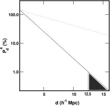
Figure 8: Probability to detect a common underdense region of size $d\ h^{-1}$ Mpc along four lines of sight in spectra with random distributions of absorption lines. Spectra with randomly placed lines were computed for 10000 quadruplets. Wavelength range and S/N ratio are the same as in the observed spectra. The corresponding probability for the occurence of underdense regions in a single line of sight is shown as dotted line. Probabilities larger than 100% correspond to more than one false detection. A 12.5 $h^{-1}$ Mpc underdense region was detected in the observed quadruplet; a larger underdense region would occur at random with a probability $\simeq 2$% (gray region).

Figure 9: The spectra of the close quadruplet of quasars, Fig. 2, centered on a common under-dense region are plotted in the four lower panels. Under-dense regions are defined as segments where the flux is everywhere higher than the average flux (solid horizontal line). The individual under-dense regions are shown with dashed vertical lines while the common region is shown with solid vertical lines. The same feature is highlighted in the upper panel where the four spectra are over-plotted: solid line for Q0102-2931; dashed line for Q0103-294a; dotted line for Q0103-294b; dot-dashed line for Q0102-293.

The previous analysis did not take into account the relative positions of the quasars in the sky. In the following, we consider underdense regions in 3D. To detect an underdense region in Galaxy surveys (e.g. Hoyle & Vogeley 2001), the void finding algorithm normally identifies walls of galaxies with a friend-to-friend algorithm. A void is then defined as the largest sphere that may be included inside one connected region. Contrary to galaxy surveys, we do not have a complete map of the high density regions, but individual underdense regions are fully defined along one line of sight, whereas galaxy surveys are limited by some magnitude threshold. We therefore search for the smallest underdense region that includes four (in the case of a quadruplet) individual underdense regions. This is equivalent to the requirement that the surface of the underdense region matches the eight edges of the four segments. To formalize this procedure, the position of each line of sight is defined as $\left(x_{{\rm l}_{\rm i}},y_{{\rm l}_{\rm i}}\right)$, with the subscript i running from 1 to 4. If the 3D surface of the underdense region satisfies $V(x,y,z)=0$, then the above requirement can be written as:

$$\mbox{for ${\rm i}=1,4$}\ \left\{\begin{array}[]{l}V(x_{{\rm l}_{\rm i}},y_{{\rm l}_{\rm i}},{\lambda_{\rm b}}^{{\rm j}_{\rm i}}\pm{\rm d}\lambda)=0\\ V(x_{{\rm l}_{\rm i}},y_{{\rm l}_{\rm i}},{\lambda_{\rm e}}^{{\rm j}_{\rm i}}\pm{\rm d}\lambda)=0\end{array}\right.\,,$$ (12)

where [${\lambda_{\rm b}}^{{\rm j}_{\rm i}},\ {\lambda_{\rm e}}^{{\rm j}_{\rm i}}$] defines a set of four individual underdense regions as defined by Eq. 11. We allow for a variation of ${\rm d}\lambda=5$Å in the position of the surface along each line of sight. This takes into account the fact that observations are in redshift space - the border of the underdense region may have a peculiar velocity that shifts its position in wavelength, and that a real underdense region has probably not a simple boundary surface. The pair Q0102-294A/B is close and highly correlated. If the constraint given by Eq. 12 is fulfilled for either of the two lines of sight, it will also be so for the other. Therefore only six real constraints remain. This set of equations can constrain a sphere that has four degrees of freedom. For simplicity we therefore search for spherical underdense regions. Inside the sphere, the intergalactic medium will be under-dense along each line of sight and on its surface it will be over-dense at eight positions identifying the edges of the individual underdense regions (the $\lambda_{\rm b}\ \mbox{and}\ \lambda_{\rm e}$).

When we applied this procedure to the observed quadruplet only one spherical underdense region was detected. It is located at the position of the common underdense region described above. The radius of the sphere is also 12.5 $h^{-1}$ Mpc. A schematic three dimensional view of this sphere and the four lines of sight is shown in Fig. 10. The projection of this 3D-view in the transverse plane shows that the four lines of sight do not probe the total size of the underdense region in the transverse direction. The geometrical configuration of the quadruplet does not allow us to discriminate between an ellipse and a sphere.

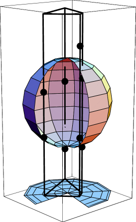
Figure 10: A schematic three dimensional representation of the sphere that contains a common underdense region along a quadruplet of quasars whose spectra are shown in Fig. 9. The position of this sphere was found with a search algorithm for three dimensional spherical underdense region (see text for details). The individual underdense regions along each line of sight are marked by the black dots.

6 Conclusion

We have analysed the Lyman-$\alpha$ forest spectra of a sample of close pairs of quasars (separations from 0.6 to 10 arcmin). We concentrated on extracting information contained in the measured correlation between the Lyman-$\alpha$ forest absorption in adjacent lines of sight. The geometrical configuration of a quadruplet with maximum separation of 10 arcmin contained in the sample has allowed us to search directly for three dimensional structures in the intergalactic medium.

1. We have detected a 12.5 $h^{-1}$ Mpc region where the absorption is everywhere below the average value, and which is present in all four spectra of the quadruplet of quasars contained in our sample. The individual regions devoid of absorption lines have a length of 21, 21, 25 and 13 $h^{-1}$ Mpc, respectively. Only 2 % of a sample of synthetic spectra with randomly distributed absorption lines have shown an underdense region of this size or larger by chance. Note that other possible interpretations include the signature of feedback from proto-clusters (e.g. Theuns, Mo & Schaye 2001) or a local increase in the UV radiation due to the presence of a nearby source (e.g. Savaglio, Panagia & Padovani 2002). We also developed a procedure to fit a set of close lines of sight  with spherical under-dense regions. With this algorithm the four regions devoid of lines define a three dimensional structure of radius 12.5 $h^{-1}$ Mpc.

2. Our sample of pairs probes a large range of angular separations, allowing a more accurate determination of the transverse correlation function than previous studies. Amplitude and shape of the transverse correlation function can be reasonably well determined up to a separation of 2-3 arcmin. At separations larger than 5-6 arcmin the correlation falls below the level which could be detected from a single pair of quasars. The measured transverse correlation function at scales smaller than 3 arcmin is consistent with expectations of CDM-like models of structure formation, where the gas is predicted to be correlated up to separation of a few Mpc. At larger scales no positive correlation is detected and the measurements may even indicate a weak anti-correlation which would not be consistent with the idea that the opacity distribution traces the DM distribution in a simple manner (cf Meiksin & Bouchet 1995). This is most likely due to the fact that our sample is still too small to detect the weak correlation expected on these scales. A larger sample is needed to clarify the situation. We have also measured the longitudinal correlation function and found similar results as other authors. The measured correlation function has a well defined shape out to a separation of $350-500$ km s^-1. While measured transverse separations are directly related to physical distances, measured line of sight separations are affected by peculiar velocities. Nevertheless the measured transverse and longitudinal correlation functions have similar shape and correlation length for reasonable choices of cosmological parameters. The longitudinal correlation function must thus indeed measure spatial density correlation on scales of a few Mpc as expected if the fluctuating Gunn-Peterson effect due to the filamentary and sheet-like structures predicted by CDM-like cosmogonies is responsible for the Lyman-$\alpha$ forest.

3. We have investigated the possibility of using a quantitative comparison of the transverse and longitudinal correlation functions (a modified version of the Alcock & Paczyński test) to constrain $\Omega_{\Lambda}$. At larges scales ($>$2 arcmin, $>350$ km s^-1) the density field is in the linear regime. We have thus modelled the peculiar velocities using linear theory for the evolution of density fluctuations. The linear theory predictions have been fitted simultaneously to the transverse and longitudinal correlations of the flux distribution and the procedure has been tested on numerical simulations. The current data set is not yet large enough to give significant constraint on $\Omega_{\Lambda}$. However, application of the test to simulated spectra of 30 pairs at 2, 4.5 (and 7.5) arcmin recovered the correct value of $\Omega_{\Lambda}\pm 0.1$ in 95% of the realizations. If the expected weak correlation at scales larger than 3 arcmin can indeed be detected in larger samples of QSO pairs a more sophisticated analysis making more extensive use of numerical simulation should deliver very significant constraints on cosmological parameters. Careful calibration with numerical simulations may also allow to exploit the much stronger correlations in the non-linear regime at scales smalller than two arcmin.

Acknowledgements: This work was supported in part by the European RTN program ”The Physics of the Intergalactic Medium”

P. Petitjean and E. Rollinde thank the Inter University Center for Astronomy and Astrophysics of Pune (IUCAA, India), the National Center for Radio Astronomy, TIFR of Pune (NCRA, India), the Astrophysikalisches Intitut Potsdam (AIP, Germany) and the Institute of Astronomy of Cambridge (IoA, UK) and M. Haehnelt thanks the Institut d’Astrophysique de Paris (IAP, France) for hospitality during the time part of this work was completed.

We thank E. Thiébaut, and D. Munro for freely distributing his Yorick programming language (available at ftp://ftp-icf.llnl.gov:/pub/Yorick) which we used to implement our algorithm.

The computational means (NEC-5x5) to do the N-body simulation were made available to us thanks to the scientific council of the Institut du Développement et des Ressources en Informatique Scientifique (IDRIS).

We also thank the anonymous referee for useful comments.

References

- [1] Alcock C., Paczyński B., 1979, Nature, 281, 358
- [2] Aracil B., Petitjean P., Smette A., Surdej J., Mücket J.P., Cristiani S., 2002, A&A, 391, 1
- [3] Bechtold J., Crotts A.P.J., Duncan R.C., Fang Y., 1994, ApJ, 437, L83
- [4] Bi H., Davidsen A.F, 1997, ApJ, 479, 523
- [5] Bond J. R., Wadsley J. W., 1998, in eds P. Petitjean, S. Charlot, XIII IAP Workshop, Editions Frontières, Paris, p. 143
- [6] Carswell R.F., Rees M. J., 1987, MNRAS, 224, 13
- [7] Cen R., Miralda-Escudé J., Ostriker J.P., Rauch M., 1994, ApJ, 437, L9
- [8] Charlton J.C., Anninons P., Zhang Y., Norman M.L., 1997, ApJ, 485, 26
- [9] Cristiani S., D’Odorico S., Fontana A., Giallongo E., Savaglio S., 1995, MNRAS, 273, 1016
- [10] Cristiani S., D’Odorico S., D’Odorico V., Fontana A., Giallongo E., Savaglio S., 1997, MNRAS, 285, 209
- [11] Croft R., Weinberg D., Bolte M., Burles S., Hernquist L., Katz N., Kirkman D., Tytler D., 2002, ApJ, 581, 20
- [12] Crotts A.P.J., 1987, MNRAS, 228, 41
- [13] Crotts A.P.J., 1989, ApJ, 336, 550
- [14] Crotts A.P.J., Fang Y., 1998, ApJ, 502, 16
- [15] Dinshaw N., Impey C.D., Foltz C.B., Weymann R.J., Chaffee F.H., 1994, ApJ, 437, L87
- [16] Dinshaw N., Foltz C.B., Impey C.D., Weymann R.J., Morris S.L., 1995, Nature, 373, 223
- [17] D’Odorico V., Cristiani S., D’Odorico S., Fontana A., Giallongo E., Shaver P., 1998, A&A, 339, 678
- [18] D’Odorico V., Petitjean P., Cristiani S., 2002, A&A, 390, 13
- [19] Efstathiou G., Bond J.R., White S.D.M., 1992, MNRAS, 258, 1
- [20] Eke V.R., Cole S., Frenk C.S., 1996, MNRAS, 282, 263
- [21] Fang Y., Duncan R.C., Crotts A.P.S., Bechtold J., 1996, ApJ, 462, 77
- [22] Hernquist L., Katz N., Weinberg D.H., Miralda-Escudé J., 1996, ApJ, 457, L51
- [23] Hoyle F., Vogeley M.S., 2001, AAS, 198, 7
- [24] Hui L., 1998, ApJ, 516, 519
- [25] Hui L., Gnedin, Y., 1997, MNRAS, 292, 27
- [26] Hui L., Stebbins A., Burles S., 1999, ApJ, 511, L5
- [27] Kaiser N., 1987, MNRAS, 227, 1
- [28] Khare P., Srianand R., York D.G., Green R., Welty D., Huang K., Bechtold J., 1997, MNRAS, 285 167
- [29] Kim T., Hu E.M., Cowie L., Songaila A., 1997, AJ, 114,1
- [30] Kim T., Cristiani S., D’Odorico S., 2001, A&A, 373, 757
- [31] Kim T., Carswell R. F., Cristiani S., D’Odorico S., Giallongo E., 2002, MNRAS, 335, 555
- [32] Liske J., Webb J.K., Williger G.M., Fernández-Soto A., Carswell R.F., 2000, MNRAS, 311, 657
- [33] Mc Donald P., Miralda-Escudé J., 1999, ApJ, 518, 24
- [34] Mc Gill C., 1990, MNRAS, 242, 544
- [35] Matsubara T., Suto Y., 1996, ApJ, 471, L1
- [36] Meiksin A., Bouchet F.R., 1995, ApJ, 448, L88
- [37] Miralda-Escudé J., Cen R., Ostriker J.P., Rauch M., 1996, ApJ, 471, 582
- [38] Mücket J.P., Petitjean P., Kates R., Riediger R., 1996, A&A, 308, 17
- [39] Ostriker J.P., Bajtlik S., Duncan R.C., 1988, ApJ, 327, L35
- [40] Petitjean P., Mücket J. P., Kates R. E., 1995, A&A, 295, L9
- [41] Petitjean P., Surdej J., Smette A., Shaver P., Mücket J., Remy M., 1998, A&A, 334, L45
- [42] Petry C.E., Impey C.D., Katz N.S., Weinberg D.H., Hernquist L.E., 2001, AAS, 199, 131
- [43] Pichon C., Vergely J.L., Rollinde E., Colombi S., Petitjean P., 2001, MNRAS, 326, 597
- [44] Rollinde E., Petitjean P., Pichon C., 2001, A&A, 376, 28
- [45] Sargent W.L.W., Young P.J., Boksenberg A., Tytler D., 1980, ApJS, 42, 41
- [46] Savaglio S., Panagia N., Padovani P., 2002, ApJ, 567, 702
- [47] Smette A., Surdej J., Shaver P.A., Foltz C.B., Chaffee F.H., Weymann R.J., Williams R.E., Magain P., 1992, ApJ, 389, 39
- [48] Smette A., Robertson J.G., Shaver P.A., Reimers D., Wisotzki L., Koehler T., 1995, A&AS, 113, 199
- [49] Theuns T., Leonard A., Efstathiou G., Pearce F.R., Thomas, P.A., 1998, MNRAS, 301, 478
- [50] Theuns T., Mo H.J., Schaye J., 2001, MNRAS, 321,450
- [51] Viel M., Matarrese S., Mo H.J., Haehnelt M.G., Theuns T., 2002, MNRAS, 329, 848
- [52] Weinberg S., 1972, Gravitation and Cosmology, New York, John Wiley, Sons
- [53] Williger G.M., Smette A., Hazard C., Baldwin J.A., Mc Mahon R.G., 2000, ApJ, 532, 77
- [54] Young P.A., Impey C.D., Foltz C.B., 2001, ApJ, 549, 76Y
- [55] Zhang Y., Anninos P., Norman M.L., 1995, ApJ 453, L57