CMBEASY:: an Object Oriented Code for the Cosmic Microwave Background

Abstract

We have ported the cmbfast package to the C++ programming language to produce cmbeasy, an object oriented code for the cosmic microwave background. The code is available at www.cmbeasy.org. We sketch the design of the new code, emphasizing the benefits of object orientation in cosmology, which allow for simple substitution of different cosmological models and gauges. Both gauge invariant perturbations and quintessence support has been added to the code. For ease of use, as well as for instruction, a graphical user interface is available.

I Introduction

The cmbfast computer program for calculating cosmic microwave background (CMB) temperature and polarization anisotropy spectra, implementing the fast line-of-sight integration method, has been publicly available since 1996 Seljak:1996is . It has been widely used to calculate spectra for open, closed, and flat cosmological models containing baryons and photons, cold dark matter, massless and massive neutrinos, and a cosmological constant. It is a very well-tested program that has enabled many cosmologists to compare models of the Universe against the experimental CMB data.

However, from the point of view of code design, there are few programs that could not be improved. This is also true for cmbfast: it is a rather monolithic code that is quite difficult to oversee and modify. For example, variations in the cosmic expansion history due to dark energy necessitate similar changes to the code in numerous separate locations.

In order to address these shortcomings and simplify modifications of the code – in our case the implementation of quintessence models and gauge invariant variables – we have ported the cmbfast package to the C++ programming language. The C++ language is object oriented and it turns out that to think in objects (more of this soon), is very advantageous in cosmology.

The program has not been rewritten from scratch, but redesigned step by step. Some people may argue that it is hence not independent, i.e. some unknown errors and limitations in cmbfast could be present in the new code. The object oriented modular design, however, ensures that each part of the code is independently testable. If, for instance, one does not trust the integrator, one can use another one to check it, without changing anything else in the package. In addition most of the lines in the code have been rewritten, to benefit from the redesign.

cmbeasy calculates the temperature and polarization anisotropies for spatially flat universes, containing dark energy, dark matter, baryons and neutrinos. The dark energy can be a cosmological constant or quintessence. There are three scalar field field models implemented, or alternatively one may specify an equation-of-state history. Furthermore, the modular code is easily adapted to new problems in cosmology.

In the next section II.1 we explain object oriented programming and its use in cosmology. The design of cmbeasy is presented in section II.2, while the graphical user interface is discussed in section II.3. Computing precision is discussed in section II.4, while the documentation for cmbeasy is introduced in II.5. For an introduction to perturbation theory and CMB physics using the conventions of cmbeasy, as well as a summary of the evolution equations, please see the documentation on www.cmbeasy.org.

II The code

We briefly introduce the concept of object oriented programming before turning to the design of cmbeasy. We do this using examples from the code.

II.1 Objects

In C++, a class is a user-defined data type stroustrup . As with any data type, there can be many variables with the same type, e.g. floats, arrays, complex numbers. In the case of user-defined types, the specific variables are called objects.

II.1.1 Encapsulation

Quite often, some data and functions acting on the data are so tightly connected, that it is sensible to think of them as one object. As an example, let us discuss splines. Given a discrete set of $n$ points $x_{i}$ with $x_{i}<x_{i+1}$ and corresponding $f(x_{i})=y_{i}$, a spline can smoothly interpolate, i.e. give $f(x)$ for any $x\in[x_{0},x_{n}]$. Provided that the sampling is dense enough, arbitrary functions may be described by a spline for all practical purposes. This is widely used in cmbfast. For instance, the $C_{l}$’s are calculated only every $50$ l-values for $l>200$. As the spectrum is very smooth, this still gives a precise result.

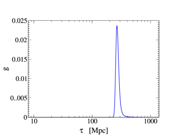
Now, the function describing the photon visibility (see also Figure 1), calculated in the part of the code that tracks the thermal history of the Universe, can be used to define a spline. Without object orientation, one would need to keep track of various variables, most notably arrays for the $x,y$ data and derivatives needed for spline interpolation. Also, in order to assure quick access within the spline data table, one either needs to know the precise layout of the data arrays (cmbfast does this), or even more variables (storing for instance the last interpolation $x$ value) would be necessary. In total, this sums up to a lot of bookkeeping for a conceptually simple entity like a spline.

Figure 1: The visibility $g\equiv\dot{\kappa}\exp(\kappa(\tau)-\kappa(\tau_{0}))$ as a function of conformal time $\tau$ in Mpc. Its peak at about $\tau\approx 300\,\textrm{Mpc}$ defines the epoch of last scattering. Before the visibility function peaks, photons are very likely to scatter again until the Universe becomes translucent. After the peak, photons do not scatter at a substantial rate. It is thus the balance between frequent scattering and sufficiently low optical depth that will give the largest contribution towards the anisotropy today. And this fact is exactly encoded in $g$.

Alternatively, one may define a class holding all the necessary variables a spline needs, together with definitions of an interface with which other parts of the program can access and manipulate the spline data. An object behaves as described by the corresponding class. There can be an arbitrary number of objects of a certain class (just like there is one floating point type float, but many variables of type float in a program). The class (in our case) called Spline, can hence be viewed as yet another data type, with no more bookkeeping needed than say for a floating point number. To illustrate this, let us discuss the visibility function $g\equiv\dot{\kappa}\exp(\kappa(\tau)-\kappa(\tau_{0}))$, where $\kappa(\tau)$ is the optical depth. Its typical shape is depicted in Figure 1, and its peak defines the epoch of last scattering. As soon as the Spline called visibility has been given the data, its maximum can be determined by a single line of code:
tau_ls = visibility.maximum();
Here, the function maximum() acts on the visibility. The important point to notice is that all functions defined in the Spline class are immediately available to everyone who uses Splines. So, whenever one needs to find the maximum, integrate a spline, calculate the convolution of two Splines etc, this can be done using very few lines of code: the functionality is fully encapsulated in the implementation of the Spline class. Any increase in performance or sophistication of the Spline class immediately translates over to all Splines used in the program.

II.1.2 Inheritance

Tightly connected to the fact that data and methods are combined within one object, is the concept of inheritance, which proves very powerful in cosmology. A class can inherit from another class (in this context called base class). All variables and the full functionality that the base class implements are instantly available to the inheriting class, called sub-class. The sub-class can then re-implement functions of the base class to provide a different functionality, or add new functions and variables. The important point to note is that all classes deriving from the same base class necessarily need to provide all the functions the base class provides. Hence, whenever the code uses the base class, one can substitute an inheriting class for the base class by simply changing one line of code.

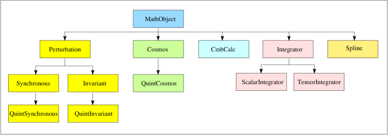
As an illustration, let us look at the Perturbation class of cmbeasy which is designed to evolve the perturbation equations for one $k$-mode through conformal time and calculate the anisotropy sources. The Perturbation class defines functions to do these calculations which other parts of the program can be sure to find implemented in all sub-classes. In practice, there are four classes that inherit from it, for perturbations in gauge-invariant variables and in synchronous gauge both with and without quintessence (see also Figure 2). From the point of view of the rest of the program, all of them are equally well suited. Hence, when given a Perturbation object, one may e.g. ask it to initialize the perturbation variables:
perturbation->initialScalarPerturbations();
Yet, depending on the specific sub-class the object belongs to , the implementation of initialScalarPerturbations() and hence the code executed will be different. Technically this is called polymorphism.

II.2 Design

There are roughly three main steps needed to calculate the CMB anisotropy spectrum within the line of sight strategy: (1) solve the expansion and thermal background evolution, (2) propagate the perturbation equations in Fourier space, (3) map the temperature anisotropy onto the sky today. In each step, several classes work together. To illustrate the hierarchy of the most important classes, an overview is given in Figure 2. The core part of the package is the CmbCalc class. It is the scheduler calling other objects to complete all three steps. So let us turn to step (1), the expansion history of the universe.

Figure 2: Hierarchy of the main classes of the cmbeasy package. All classes dealing with mathematics inherit from MathObject for technical reasons. The Cosmos class calculates the background evolution and can be extended using subclasses such as QuintCosmos for quintessence. The perturbation equations are encapsulated in the Perturbation class. Implementing different gauges as subclasses is therefore unproblematic. The central instance invoking Cosmos, the Perturbations and Integrators is the CmbCalc class. Not shown are several (sometimes small) classes, e.g. the ControlPanel, which holds commonly used settings, or e.g. the MiscMath class providing low-level mathematical functions.

II.2.1 The background evolution

The Cosmos class is the central instance providing background quantities like the energy density $\bar{\rho}(\tau)$ of all species etc. This centralization of the background evolution within the Cosmos class facilitates the modification of the code significantly. A different background cosmology (such as quintessence) can be implemented by just inheriting from Cosmos and re-implementing the expansion history part of the code. For most other objects in the code, it makes no difference exactly what caused the universe to expand, as long as they can rely on Cosmos or any sub-class to provide access to the expansion history. Both the expansion and the thermal history are computed at the beginning of the calculation and stored in splines.

II.2.2 Propagation in k-space

All fluctuation equations are handled by Perturbation and its sub-classes. Its most prominent function is propagateScalar($\tau_{1},\,\tau_{2}$) which evolves the perturbations from conformal time $\tau_{1}$ to $\tau_{2}$. For numerical stability, one usually treats the era of tight coupling between baryons and photons differently. However, this results in a non-analytic jump in the r.h.s of the perturbation equations at $\tau_{tc}$. Some integrators for ordinary differential equations get confused by this. Therefore, propagateScalar() will determine if the jump occurs within [$\tau_{1},\,\tau_{2}$] and if so, integrate up to $\tau_{tc}$, make a tiny jump and integrate on till $\tau_{2}$. At the end of each propagation, the sources of cmb anisotropies are calculated by the scalarSources() function.

II.2.3 The Cl’s

The convolution of the sources with the Bessel functions, as well as the final $k$-integration are performed in the ScalarIntegrator sub-class. In contrast to cmbfast, we formulate the convolution with the $j_{l}^{\prime}s$ as an ordinary differential equation (ODE). In fact, the Spline class provides the convolution functionality. If higher precision in this step is wanted, one may simply increase the desired precision for Spline, which will pass this through to the integrator of ODE’s. As far as the $k$-integration is concerned, we stick to the interpolation points of cmbfast. We have written two other implementations of ScalarIntegrator, although none could compete with cmbfast’s speed. Furthermore, no gain in accuracy justifying the speed tradeoff was found. As far as the $k$-integration is concerned, a fast and independent realization would be desirable. With the high level features of C++, algorithms that seem hard to implement in other languages may be feasible.

II.2.4 Little helpers

The most valuable class assisting the computation may be Spline. As splines are used all over the code, and quite often in time-critical environments, the main design goal has been speed. In order to perform a spline interpolation at $x$, one needs to find the interval $x\in[x_{i},x_{i+1}]$. While cmbfast  hard-wires the size and layout of the $x_{i}$-data, this has not been an option for a versatile spline implementation. Yet, in all time critical situations within our calculation, two facts come to the rescue: Firstly, interpolations occur in order and close to the last interpolation. Hence, the next value of $x$ is likely to lie within the same interval (or close to it). Secondly, many splines with exactly the same $x$-data are evaluated at the same $x$. For instance, the r.h.s of the perturbation equations need background quantities all at the same $\tau$. As all background quantities get their data at the same $\tau_{i}$ in Cosmos, they necessarily share the same $x$-data. Therefore, some parts of the interpolation formulae have to be computed only once for each $\tau$. In addition, finding the position of the interpolation interval is simple: it will be the same for the same $\tau$.

To accommodate for these groups of splines and caching, splines come in two flavors: with and without its own $x$-data. While a spline with its own $x$-data can live on its own, a spline without $x$-data can only be created if a “mother” spline providing the $x$-data is given upon the creation of the “child” spline. Within these “families” of shared $x$-data, interpolation at the same $x$ is particularly fast.

Not only must a spline be fast, it must also be robust. Hence, a spline will allocate more memory if needed, check that no access to data occurs outside its bound, check that all data is ordered $x_{i}<x_{i+1}$ and make sure that the interpolation tables have been built before any interpolation takes place. Splines can easily be visualized. To write the data to a file, simply call
myspline.dump("filename")
The anisotropy sources, are evaluated on a $\{k,\tau\}$ grid. For the final $\tau$ and $k$ integration, one needs to interpolate at intermediate points. This is conveniently done using the class SplineWeb. It is essentially an array of Splines, one for each $k$ and one for each $\tau$ value. If one needs to interpolate at a given $k$ value, one can ask SplineWeb to return a Spline with x-data in the $\tau$ direction:
spline_at_k = web.createAlongY(k);
This is used to get the splines which are convoluted with the Bessel functions. It is also very convenient for making slices through the cold dark matter power spectrum (at either fixed $k$ or $\tau$). Given for instance the cold dark matter SplineWeb power, one can dump it to a file:
power.dumpAlongX($\tau$,"filename");
The above command would save the spectrum at arbitrary conformal time $\tau$ to disk.

There are some more of these “helpers”, most of them small classes that sometimes make life much easier. The last one we will introduce here is Anchor which keeps track of objects that are dynamically created (as are many splines). The objects it is asked to keep track of are deleted by it on demand, or when the Anchor object itself is deleted. Therefore, it greatly simplifies memory handling and prevents memory leaks.

II.2.5 Quintessence Implementation

The different background evolution of quintessence Wetterich:1988fm ; Ratra:1988rm ; Caldwell:1998ii scenarios is implemented using the QuintCosmos and the Quintessence class. Each subclass of Quintessence corresponds to a certain model, such as the exponential potential Wetterich:1988fm ; Peebles:1988ek ; Ratra:1988rm , inverse power law Ratra:1988rm , leaping kinetic term Hebecker:2001zb etc. Certainly, a more monolithic design with the quintessence models implemented in the QuintCosmos class would have been possible. However, we believe that the details of a model are best kept to a class of its own. For instance tuning model parameters in order to get the right amount of $\Omega_{0}^{\varphi}$ is different for each model and a monolithic design would have to call differently named functions for different models. Using sub-classing, QuintCosmos (and Perturbation) always calls functions with the same argument and name for all models. Yet, as the object implementing the function differs for each model, the code executed by calling the function can be totally different. Thus, a new quintessence model can be implemented by simply sub-classing Quintessence and implementing a minimal set of functions, such as one for the scalar field potential.

Figure 3: Graphical user interface (GUI) for cmbeasy.

II.3 Graphical User Interface

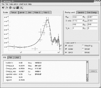
For educational purposes and also to simplify the parameter input and subsequent visualization of results, a graphical user interface (GUI) is of great value. Luckily, there is the very sophisticated and publicly available ‘Qt’ library troll with which the creation of a GUI is facilitated. Its object oriented C++ design is a perfect match for the cmbeasy package. There is therefore an executable program called ‘cmbeasy’ giving interactive access to almost the full capabilities of the package, including quintessence. As is seen from Figure 3, the spectra are visualized in separate plots arranged in a so called Tab-Widget. One can for instance zoom in, select and save curves or print the plot.

II.4 Computing precision

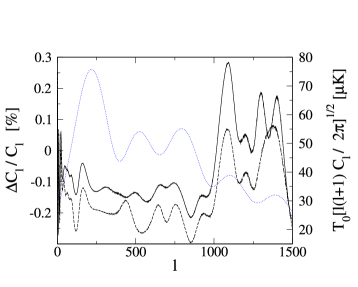
Comparing the results from cmbfast to those obtained from cmbeasy, one generally notes accordance to better than $0.5\%$ (see also Figure 4).

In principle, the line of sight algorithm is equivalent to evolving a large hierarchy of multipoles. In practice, as one truncates the hierarchy in the line of sight approach at some low $l$, there is a reflection of power after the higher multipoles gradually build up. However, as by far the largest contribution towards the anisotropy occurs around recombination (when the higher multipoles are still small), this does not spoil the result dramatically. Yet, to check this, one may increase the number of multipoles involved. This is true both for cmbfast and cmbeasy.

Within cmbeasy, there are five instances in which the precision may be increased. In three of the five cases, changing one variable suffices. The first case is the background evolution. Here one may want to increase (or decrease) the precision requested from the ODE integrator. During perturbation evolution in $k$-space, the precision requirement given to Perturbation can be changed in a similar manner. The same is true for the convolution of the sources with the Bessel functions, taking place in ScalarIntegrator. Finally, and a bit more difficult, one may change the number and position of $k$-values contributing towards the $k$-integration. This can be done by modifying Integrator, the base class of ScalarIntegrator. Alternatively, one could devise a different implementation for the $k$-integration. Finally, one may increase the number of $l$’s at which the $C_{l}$’s are calculated.

Figure 4: Temperature anisotropy spectrum for $h=0.65,\ \Omega_{0}^{\Lambda}=0.6,\ \Omega_{0}^{\rm b}h^{2}=0.02,\ \Omega_{0}^{\rm c}=1-\Omega_{0}^{\Lambda}-\Omega_{0}^{\rm b}$ obtained from cmbfast. The relative deviation $\Delta C_{l}/C_{l}$ of cmbeasy’s synchronous (long dashed line) and gauge invariant (solid line) solution with respect to the original cmbfast spectrum are also given. The accordance of all spectra is always better than $1\%$. In the gauge invariant case, both the background and perturbation evolution as well as the $C_{l}$ integration are entirely independent of the cmbfast code. However, they use the same thermal history algorithm that should in principle be independently implemented for cross checks.

II.5 Documentation

Using the doxygen program, the documentation is automatically generated from the source code of the cmbeasy package. In its html version, it is interactively navigable and includes the full source code. Due to the automatic generation, the documentation and the code are naturally synchronized. Instructions for setting up and running the program are available in this html documentation. In addition, a postscript version of the documentation is generated.

III Conclusions

We have devised an object oriented code for calculating cosmic microwave background anisotropies. The main benefits of this code derive from its modularity.

The modular design allows one to test and refine each part of cmbeasy individually. Different modules, for different numerical methods and theoretical approaches, can easily be switched. This feature should prove extremely useful in the development and refinement of the code. As cosmological theory reaches for a new level of precision to match the new generation of experiments, map MAP , planck PLANCK and other experiments will soon put our predictions and hypotheses to the test, so future work will seek to improve the accuracy of the code. (At the present time, cmbeasy  and the standard cmbfast are generally in agreement to better than $0.5\%$.)

The modular design allows one to more easily develop and build upon cmbeasy, to implement new cosmological models and include more physics. As our theoretical cosmological models are a work-in-progress — as CMB data comes in — so are our tools for modeling the Universe. And so it makes sense to use a program design which makes this development easy. Hence, the functional blocks used in cmbeasy  considerably reduce the time to implement new cosmological models. For most purposes, a new model can be achieved by sub-classing from existing solutions, thus eliminating the need to rewrite large parts of the code. Furthermore, new modules can be easily introduced to carry out calculations that rely on the linear perturbation spectrum. Examples include lensing, secondary sources in the CMB, reionization, and cross-correlation with other tracers of large scale structure.

An additional benefit of the cmbeasy  package is the graphical front-end. As we have described, the GUI allows a user to visually dial through a range of parameters. We expect that this functionality will be useful for developing understanding and intuition for CMB physics and cosmological models.

As stated at the outset, there is, perhaps, no program design that could not be improved. However, we hope that cmbeasy will serve the cosmology community well.